Information correlated L evy walk exploration and distributed mapping using a swarm of robots - arXiv
←
→
Page content transcription
If your browser does not render page correctly, please read the page content below
1

                                            Information correlated Lévy walk exploration and
                                               distributed mapping using a swarm of robots
                                                                           Ragesh K. Ramachandran1 , Zahi Kakish2 , and Spring Berman2

                                            Abstract—In this work, we present a novel distributed method               into the following approaches. Feature-based mapping [2],
                                         for constructing an occupancy grid map of an unknown environ-                 also known as landmark-based mapping, is a method in
                                         ment using a swarm of robots with global localization capabilities            which the environment is represented using a list of global
                                         and limited inter-robot communication. The robots explore the
                                                                                                                       positions of various features or landmarks that are present in
arXiv:1903.04836v3 [cs.RO] 18 Jun 2020

                                         domain by performing Lévy walks in which their headings
                                         are defined by maximizing the mutual information between the                  the environment. Consequently, the algorithms in this category
                                         robot’s estimate of its environment in the form of an occupancy               require feature extraction and data association. Occupancy
                                         grid map and the distance measurements that it is likely to obtain            grid mapping uses an array of cells to represent an unknown
                                         when it moves in that direction. Each robot is equipped with laser            environment. This class of algorithms was first introduced
                                         range sensors, and it builds its occupancy grid map by repeatedly
                                         combining its own distance measurements with map information                  in [3] and is the most commonly used method in robotic
                                         that is broadcast by neighboring robots. Using results on average             mapping applications. Occupancy grid maps are very effective
                                         consensus over time-varying graph topologies, we prove that all               at representing 2D environments, but their construction suffers
                                         robots’ maps will eventually converge to the actual map of the                from the curse of dimensionality. The cells in an occupancy
                                         environment. In addition, we demonstrate that a technique based               grid map are associated with binary random variables that
                                         on topological data analysis, developed in our previous work
                                         for generating topological maps, can be readily extended for                  define the probability that each grid cell is occupied by
                                         adaptive thresholding of occupancy grid maps. We validate the                 an object. Topological mapping [4] procedures generate a
                                         effectiveness of our distributed exploration and mapping strategy             topological map, which is a compact sparse representation
                                         through a series of 2D simulations and multi-robot experiments.               of an environment. A topological map encodes all of an
                                                                                                                       environment’s topological features, such as holes that signify
                                            Index Terms—Distributed robot system, mapping, occupancy                   the presence of obstacles, and identifies collision-free paths
                                         grid map, information theory, algebraic topology                              through the environment in the form of a roadmap. This map
                                                                                                                       is defined as a graph in which the vertices correspond to
                                                                                                                       particular obstacle-free locations in the domain and the edges
                                                                  I. I NTRODUCTION
                                                                                                                       correspond to collision-free paths between these locations.

                                         T     ECHNOLOGICAL advances in embedded systems such
                                               as highly miniaturized electronic components, as well
                                         as significant improvements in actuator efficiency and sensor
                                                                                                                          Size and cost constraints limit individual robots in a swarm
                                                                                                                       from having sufficient sensing, computation, and communica-
                                                                                                                       tion resources to map the entire environment by themselves
                                         accuracy, are currently enabling the development of large-                    using existing SLAM-based mapping techniques. In addition,
                                         scale robot collectives called robotic swarms. Swarms of                      inter-robot communication in a swarm is constrained by re-
                                         autonomous robots have the potential to perform tasks in                      stricted bandwidth and random link failures, and the mobility
                                         remote, hazardous, and human-inaccessible locations, such as                  of the robots results in a dynamically changing, possibly
                                         underground cave exploration, nuclear power plant monitoring,                 disconnected communication network. However, many exist-
                                         disaster response, and search-and-rescue operations. In many                  ing multi-robot mapping strategies are extensions of single-
                                         of these applications, a map of the environment where the task                robot techniques under centralized communication or all-to-
                                         should be performed is not available, and it would therefore                  all communication among robots. These strategies include
                                         be necessary to construct this map using sensor data from the                 approaches based on particle filters, with the assumption that
                                         robots.                                                                       robots broadcast their local observations and controls [5], and
                                            A widely-used technique for solving this problem is si-                    extensions of the Constrained Local Submap Filter technique,
                                         multaneous localization and mapping (SLAM) [1], a class                       in which robots build a local submap and transmit it to a
                                         of algorithms for constructing a map of a domain through                      central leader that constructs the global map [6].
                                         appropriate fusion of robot sensor data. The numerous algo-                      It is therefore necessary to develop mapping strategies for
                                         rithms that have been proposed for SLAM can be categorized                    robotic swarms that can be executed in a decentralized fashion,
                                                                                                                       and that can accommodate the aforementioned constraints on
                                            *This work was supported by the Arizona State University Global Security
                                         Initiative.
                                                                                                                       inter-robot communication. In addition, building a map in a
                                            1 Ragesh K. Ramachandran is with the Department of Computer Sci-           distributed manner has the advantage that a team of robots
                                         ence, University of Southern California, Los Angeles, CA 90089, USA           can exhibit more efficient and robust performance than a
                                         rageshku@usc.edu                                                              single robot. There have been numerous efforts to develop
                                          2 Zahi Kakish, and Spring Berman are with the School for Engineering of
                                         Matter, Transport and Energy, Arizona State University, Tempe, AZ 85287,      distributed techniques for multi-robot mapping. Various multi-
                                         USA zkakish@asu.edu, spring.berman@asu.edu                                    robot SLAM techniques that can be implemented on relatively
2
Since all robots ultimately arrive at a consensus on the map,
this map can be retrieved from a single arbitrary robot in the
swarm, making the strategy robust to robot failures. We also
introduce an exploration strategy that combines concepts from
information theory [16] with Lévy walks, a type of random
walk with step lengths distributed according to a power law
that has been used as a model for efficient search strategies by
both animals and robots [17]. We empirically show that this
new exploration strategy, which we refer to as an information
correlated Lévy walk (ICLW), enables a swarm of robots
to explore a domain faster than if they use standard Lévy
walks, thereby enabling them to map the domain more quickly.
Finally, we illustrate that a technique based on topological data
analysis, used for generating topological maps in our previous
work [18], can also be used for adaptive thresholding of
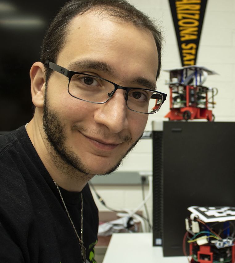
Fig. 1: A diagram of our mapping strategy. The arrows indicate occupancy grid maps with a slight modification. The threshold
information flow among components in our strategy. distinguishes occupied grid cells from unoccupied cells in
small groups of robots are surveyed in [7]. In [8], a dis- the map by applying tools from algebraic topology [19]. A
tributed Kalman filter expressed in information matrix form significant difference between our earlier topological approach
is presented and formally analyzed as a solution to distributed and the one presented in this paper is our use here of cubical
feature-based map merging in dynamic multi-robot networks. complexes [20], a natural choice for grid maps, instead of
This approach requires the robots have unique identifiers. simplicial complexes [21] We validate our mapping approach
There is also an ample literature on distributed strategies for in 2D simulations of various environments with different
occupancy grid mapping [9]–[12], which focuses on finding sizes and layouts, using the mobile robot simulator Stage
approximate relative transformation matrices among robots’ [22]. We also experimentally validate our approach with the
occupancy grid maps and fusing the maps using various commercially available TurtleBot 3 Burger robots.
image processing techniques. These strategies utilize matrix In contrast to many multi-robot strategies for exploration
multiplication operations for combining maps from different and mapping, our approach is an identity-free strategy in
robots. The most efficient algorithm for multiplying two N ×N that the robots are indistinguishable from one another; i.e.,
matrices (each representing an occupancy grid map) has a robots are agnostic to the individual identities of other robots
computational complexity of O(N 2.373 ) [13]. In comparison, with which they interact. This property is useful for map-
as we show in Section III-C, the complexity of our map- ping approaches using robotic swarms, since it facilitates the
sharing procedure is O(N 2 ) in typical cases, and is linear in scalability of the approach with the number of robots and is
the number of robots in the worst case, which occurs when robust to robot failures during task execution. In addition,
a robot communicates with all other robots during the map- unlike many multi-robot mapping strategies, our approach
sharing step. Thus, in typical cases, our approach has improved is suitable for robotic platforms with limited computational
scaling properties compared to other distributed methods for capabilities, which is a typical constraint on robots that are
occupancy grid mapping. intended to be deployed in swarms since each robot should be
In this paper, we present a distributed approach to the relatively inexpensive. Notably, although the robots identify
mapping problem that is scalable with the number of robots, other robots within their sensing range as obstacles, our
relies only on local inter-robot communication, and does not approach filters out these “false obstacles” when generating
require robots to have sophisticated sensing and computation the map of the environment from the robots’ data. Also, our
capabilities. Figure 1 gives a schematic diagram of our map- map merging approach guarantees that the map of each robot
ping strategy. In our approach, robots explore an unknown will eventually converge to the actual map of the domain, as
environment while simultaneously building an occupancy grid long as the robots’ exploration strategy facilitates sufficient
map online from their own distance measurements and from communication among the robots and coverage of the domain.
maps communicated by other robots that they encounter. As in In our previous work, we developed different techniques
most occupancy grid mapping strategies, we assume that each for addressing swarm robotic mapping problems. In [23],
robot is either capable of accurately estimating its pose or is we present a method for mapping GPS-denied environments
equipped with a localization device. We present a distributed using a swarm of robots with stochastic behaviors. Unlike
algorithm for sharing and fusing occupancy grid maps among this paper, the approach in [23] employs optimal control of
robots in such a way that each robot’s map eventually con- partial differential equation models of the swarm population
verges to the same global map of the entire environment, which dynamics to estimate the map of the environment. Although
we prove using results on achieving consensus on time-varying the method in [23] only requires robot data on encounter times
graphs [14]. Our analysis of the distributed mapping algorithm with features of interest, it is limited in application to domains
is similar, in spirit, to the ones present in [15]. The robots with a few sparsely distributed features. The methodologies
do not need to have unique identities that are recognized by discussed in our previous works [24] and [18] estimate the
other robots in order to implement this map-sharing algorithm. number of obstacles in the domain and extract a topological
3

map of the domain, respectively. Except for the procedure                                            TABLE I: Notation
for adaptive thresholding of occupancy grid maps that is             Symbol                Description
delineated in Section V, the work presented in this paper
                                                                     NR                    Number of robots
is novel and does not directly follow any of our previous            Ri                    Label of robot i ∈ {1, ..., NR }
works. Also, unlike our previous works, this mapping strategy        xi                    x-coordinate of Ri w.r.t to global frame
computes the map online rather than offline.                         yi                    y-coordinate of Ri w.r.t to global frame
                                                                     θi                    Orientation of Ri w.r.t to global frame
   In summary, the contributions of this paper are as follows:
                                                                     zτi,a                 Measurement from ath laser range sensor of Ri at time τ
   • We present a new exploration strategy for robotic swarms        xiτ                   Pose [xi yi θ i ]T of Ri at time τ
      that consists of Lévy walks influenced by information-        viτ                   Linear velocity vector of Ri at time instant τ
      theoretic metrics.                                             ziτ                   Vector of laser range sensor measurements of Ri at time τ
                                                                     Mi                    Occupancy grid map stored in Ri
   • We develop a completely decentralized strategy by which         mij                   jth grid cell of occupancy map M i
      a swarm of robots without unique identities can generate       Pmi                   Probability that cell mij is occupied (occupancy probability)
                                                                         j
      an occupancy grid map of an unknown environment.               PM i                  Probability that occupancy map M i is completely occupied
   • We prove that each robot’s occupancy grid map asymp-                                                                n     o|Mi |
                                                                     P̄M i                 Set of occupancy probabilities Pmi
      totically converges to a common map at an exponential                                                                     j       j=1
                                                                     si                    Constant speed of Ri
      rate.                                                          ∆t                    Time interval [τ τ + T ]
   • We extend our topological data analysis-based technique         Xi∆t                  Pose sequence [xiτ · · · xiτ 0 · · · xiτ+T ]
      for adaptive thresholding of occupancy grid maps [18],         Zi∆t                  Measurement sequence [ziτ , · · · , ziτ 0 , · · · , ziτ+T ]
      [24], [25] to domains represented as cubical complexes,        I[A; B|C]             Mutual information between random var.’s A, B given C
                                                                                        Arithmetic mean of the elements in vector a
      instead of simplicial complexes as in our prior work.          < a >gm               Geometric mean of the elements in vector a
   The remainder of the paper is organized as follows. Sec-          u(mij , xik , zik )   Update rule that Ri uses to assign Pmi
                                                                                                                                    j
tion II formally states the problem that we address and the          G(k)                  Undirected robot communication graph at time step k
                                                                     V                     Vertex set of G(k), {1, ..., NR } (robot indices)
associated assumptions. We describe our swarm exploration            E(k)                  Edge set of G(k) (pairs of robots that can communicate)
strategy in Section III and our occupancy grid mapping               A(k)                  Adjacency matrix associated with G(k)
strategy and its analysis in Section IV. Section V outlines our      Nik                   Neighbors of Ri (can communicate with Ri ) at time step k
TDA-based method for adaptive thresholding of occupancy
grid maps and basic concepts from algebraic topology that
are required to understand the technique. Section VI and             B. Representation of the domain as an occupancy grid map
Section VII present and discuss the results from simulations
and robot experiments, respectively. The paper concludes with           Every robot models the unknown environment as an oc-
Section VIII.                                                        cupancy grid map, which does not require any a priori
                                                                     information about the size of the domain and can be expanded
                                                                     as the robot acquires new distance measurements [1]. Each
                  II. P ROBLEM S TATEMENT                            grid cell of an occupancy grid map is associated with a value
   We address the problem of estimating the map of an un-            that encodes the probability of the cell being occupied by an
known domain D ⊂ Rd using distance measurements acquired             obstacle. Let Mti denote the occupancy grid map stored by
by a swarm of NR robots while exploring the domain. We               robot Ri at time t, where i ∈ {1, ..., NR }. We specify that each
consider bounded, closed, path-connected domains that con-           robot discretizes the domain with the same resolution. At this
tain static obstacles. Although in this paper we only address        resolution, a map of the entire domain D ⊂ R2 is discretized
the case d = 2, it is straightforward to extend our procedure        uniformly into |D| grid cells, labeled mi1 , ..., mi|D| . During the
to the case d = 3. Table I lists the definitions of variables that   mapping procedure, each robot augments its map based on its
we use throughout the paper for ease of reference.                   own distance measurements and map information from nearby
                                                                     robots, effectively adding grid cells to its current map. The
                                                                     occupancy grid map of robot i at time t is represented by the
A. Robot capabilities
                                                                     grid cells mi1 , ..., mi|Mi | , where |Mti | denotes the number of grid
                                                                                               t
   We assume that the robots have the following capabilities.        cells in the robot’s map at time t. Henceforth, we will usually
Each robot acquires noisy distance measurements using a              drop the subscript t from Mti to simplify the notation, with the
laser range sensor such as a SICK LMS200 laser rangefinder           understanding that the map M i depends on time.
[26]. Using this data, a robot can detect its distance to               Let mij , j ∈ {1, ..., |M i |}, be a Bernoulli random variable
obstacles and other robots within its local sensing radius and
                                                                     that takes the value 1 if the region enclosed by grid cell mij
perform collision avoidance maneuvers if needed. Each robot
                                                                     is occupied by an obstacle, and 0 if it is not. Thus, P(mij =
broadcasts its stored map information, and other robots that
are within a distance br of the robot can use this information       1) is the probability that grid cell mij is occupied, called its
to update their own maps. We assume that each robot can              occupancy probability. A standard assumption for occupancy
estimate its own pose with no uncertainty. It is important to        grid maps is the independence of the random variables mij . As
note that the robots are not equipped with any sensors that can      a result, the probability that map M i belongs to a domain which
                                                                                                                              |M i |
distinguish between obstacles and other robots. The robots also      is completely occupied is given by P(M i ) = ∏ j=1 P(mij = 1).
do not have unique identifiers.                                      For the sake of brevity, we will use the notation Pmi ≡ P(mij =
                                                                                                                                              j
4
1) and PMi ≡ P(M i ) throughout the paper. We also define the while covering the domain; therefore, it is an identity-free
o|Mi |
strategy.
n
set P̄Mi = Pmi , which is the collection of the occupancy
j j=1 To execute a Lévy walk, a robot repeatedly chooses a new
probabilities of all grid cells in map M i . Finally, the entropy heading and moves at a constant speed [38] in that direction
H(M i ) of the map M i , which quantifies the uncertainty in the over a random distance that is drawn from a heavy-tailed
map, is defined as [1]: probability distribution function p(l), of the form
|M i | p(l) ∝ l −α , (2)
H(M i ) = P(mij = k) log2 P(mij = k)
∑ ∑ (1)
j=1 k={0,1}
where α is the Lévy exponent. The case 1 < α < 3 signifies
a scale-free superdiffusive regime, in which the expected
displacement of a robot performing the Lévy walk over a given
C. Mapping approach and evaluation
time is much larger than that predicted by random walk models
Our mapping approach consists of the following steps. All of uniform diffusion. This superdiffusive property disperses
robots explore the domain simultaneously using the random the robots quickly toward unexplored regions.
walk strategy that is defined in Section III. While exploring, In contrast to standard Lévy walks (SLW), in which the
each robot updates its occupancy grid map with its own agent’s heading is uniformly random, we define the heading
distance measurements, broadcasts this map to neighboring chosen by the robot before each step in the Lévy walk as
robots, and then modifies its map with the maps transmitted the direction that maximizes the robot’s information gain
by these neighboring robots using a predefined discrete-time, about the environment. This is computed as the direction
consensus-based protocol, which is discussed in Section IV. that maximizes the mutual information between the robot’s
We prove that the proposed protocol guarantees that every current occupancy grid map and the distance measurements
robot’s map will eventually converge to a common map. A that it is likely to obtain when it moves in that direction,
technique for post-processing the occupancy grid map based based on the forward measurement model of a laser range
on topological data analysis (TDA) is presented in Section V. sensor [1] over a finite time horizon. These measurements
We evaluate the performance of our mapping approach accord- are expected to decrease the entropy of the robot’s occupancy
ing to two metrics: (1) the percentage of the entire domain that grid map, defined in Equation (1). Therefore, the computed
is mapped after a specified amount of time, and (2) the entropy robot heading is more likely to direct the robot to unexplored
of the final occupancy grid map, as defined in Equation (1). regions than a uniformly random heading. The calculation of
this heading is described in the following subsections.
III. E XPLORATION BASED O N I NFORMATION
C ORRELATED L ÉVY WALKS A. Laser range sensor forward measurement model
In this section, we describe the motion strategy used by We assume that the laser range sensor of each robot Ri
robots to explore the unknown domain. Exploration strate- has Nl laser beams that all lie in a plane parallel to the base
gies for robotic swarms generally use random, guided, or of the robot. The distance measurement obtained by the ath
information-based approaches [1], [9], [27], [28]. Random laser beam of robot Ri at time τ is a random variable that
exploration approaches are often based on Brownian mo- will be denoted by zτi,a . The random vector of all distance
tion (e.g., [29]–[31]) or Lévy walks (e.g., [17], [32]–[35]), measurements obtained by robot Ri at time τ is represented
i,Nl T
which facilitate uniform dispersion of the swarm through- as ziτ = [zτi,1 · · · zi,a
τ · · · zτ ] .
out a domain from any initial distribution. Moreover, these Define smin and smax as the minimum and maximum possible
approaches do not rely on centralized motion planning or distances, respectively, that can be measured by the laser
extensive inter-robot communication, which can scale poorly range sensor. In addition, let δ denote the actual distance
with the number of robots in the swarm. Information-based of an obstacle that is intersected by the ath laser beam of
approaches, such as [36], [37], guide robots in the direction robot Ri . The Gaussian distribution function with mean µ
of maximum information gain based on a specified metric, and variance σ 2 will be written as N (µ, σ 2 ). We define the
which can increase the efficiency of exploration compared to probability density function of the distance measurement zi,a
τ ,
random approaches. Mutual information (or information gain), given the actual distance δ , as the forward measurement model
a measure of the amount of information that one random presented in [36],
N (0, σ ),
variable contains about another [16], is a common metric used 2 δ ≤ smin
to assess the information gain that results from a particular i,a
P(zτ | δ ) = N (smax , σ ), δ ≥ smax
2 (3)
action by a robot. This metric can be used to predict the
N (δ , σ ),
2 otherwise,
increase in certainty about a state of the robot’s environment
that is associated with a new sensor measurement by the robot. where σ 2 is the variance of the range sensor noise in the radial
We specify that each robot in the swarm performs a direction of the laser beam. Although this model does not
combination of random and information-based exploration ap- incorporate range sensor noise in the direction perpendicular
proaches, in order to benefit from the advantages of both types to the laser beam, the experimental results in [36] and our
of strategies. We describe the implementation of ICLW in this results in Section VII demonstrate that the model captures
section. Our exploration strategy does not require the robots to sufficient noise characteristics for generating accurate maps
identify or use any information from their neighboring robots from the sensor data.
5

B. Robot headings based on mutual information                                      function in Equation (4) tends to direct a robot to unexplored
   The mutual information between two random variables A                           regions according to its current map. By the definition of
and B is defined as the Kullback-Leibler distance [16] between                     mutual information (see Equation (7)), I[M i ; Zi∆t | Xi∆t ]
their joint probability distribution, P(A, B), and the product of                  quantifies the expected reduction in the uncertainty of a robot’s
their marginal probability distributions, P(A)P(B):                                map due to the sensor measurements received by the robot
                                                                                   during its motion. In essence, I[M i ; Zi∆t | Xi∆t ] captures the
                I[A; B] = KLD (P(A, B)||P(A)P(B))                           (4)    expected amount of entropy reduced in the robot’s map M i
                                                                                   based on the likely measurements (Zi∆t ) that the robot would
This quantity measures how far A and B are from being
                                                                                   obtain if it followed a trajectory Xi∆t . Therefore, maximizing
independent. In other words, I[A; B] quantifies the amount
                                                                                   I[M i ; Zi∆t | Xi∆t ] for different trajectories (Xi∆t ) yields the tra-
of information that B contains about A, and vice versa. For
                                                                                   jectory that decreases the uncertainty in the robot’s map by the
example, if A and B are independent random variables, then
                                                                                   largest amount. There is an equal chance for a grid cell in an
no information about A can be extracted from the outcomes of
                                                                                   unexplored region to be free or occupied by an obstacle. Since
B, and consequently, I[A; B] = 0. On the other hand, if A is a
                                                                                   the entropy of a Bernoulli random variable is highest when its
deterministic function of B, then the entropies of both random
                                                                                   probability of occurrence is 0.5, the occupancy probabilities
variables are equal to the expected value of − log2 (P(A)), and
                                                                                   of the grid cells in the unexplored region have the highest
I[A; B] is equal to this quantity, which is its maximum value.
                                                                                   entropy (uncertainty). Thus, maximizing I[M i ; Zi∆t | Xi∆t ] will
   During each step in its random walk, every robot performs
                                                                                   generate trajectories that direct the robot toward unexplored
the following computations and movements. A new step may
                                                                                   regions based on the information contained in its map.
be initiated either when the robot completes its previous step,
or when the robot encounters an obstacle (or other robot)
during its current step. Suppose that the next step by robot                       C. Computing mutual information
Ri starts at time τ. At this time, the robot computes the                              In this section, we describe the computation of the objective
duration T of the step by generating a random distance based                       function in Equation (5) and discuss techniques for solving the
on the Lévy distribution (Equation (2)) and dividing this                         associated optimization problem. We first focus on computing
distance by its speed si , which is constant. Also at time τ,                      I[M i ; zi,a
                                                                                            τ ], the mutual information between the measurement
the robot computes the velocity vi∆t that it will follow during                    zi,a                       th                          i
                                                                                    τ obtained by the a laser beam of robot R at time τ and
the time interval ∆t := [τ τ + T ]. This computation involves                                                                         i
                                                                                   the robot’s current occupancy grid map M . Grid cells in the
several variables, which we introduce here. The pose of robot                      map that do not intersect the beam do not to contribute to the
Ri at time τ is denoted by xiτ (see Table I). We define a                          mutual information. Hence, the task of computing I[M i ; zi,a    τ ]
sequence of this robot’s poses during the time interval ∆t                         reduces to computing I[ci,a         i,a           i,a
                                                                                                                  τ ; zτ ], where cτ is the collection
as Xi∆t := [xiτ · · · xiτ 0 · · · xiτ+T ], where τ 0 ∈ ∆t. We also                 of Bernoulli random variables mij modeling the occupancy of
define Zi∆t := [ziτ , · · · , ziτ 0 , · · · , ziτ+T ] as a set of random vectors   grid cells in the map of robot Ri that are intersected by the
modeling laser range sensor measurements that the robot is                         ath beam at time τ. This quantity is defined as [39]:
expected to receive as it moves during this time interval. At
                                                                                                                                     P(c, z)
                                                                                                       Z
                                                                                             i,a i,a
time τ, robot Ri calculates its velocity vi∆t as the solution                            I[cτ ; zτ ] =               P(c, z) log2              dz, (6)
                                                                                                           i,a ∑
∗ vi to the following optimization problem, with the objective                                          z∈zτ     i,a                P(c)P(z)
   ∆t                                                                                                        c∈cτ
function defined as in [36], [39] :
                                                                                   where P(c, z) is the joint probability distribution of c and
           ∗ i                               I[M i ; Zi∆t | Xi∆t ]                 z, and P(c) and P(z) are the probability distributions of the
            v∆t =        arg max                                   ,        (5)
                  kvi∆t k=si , ∠vi∆t ∈[−π,π]        C(vi∆t )                       occupancy probabilities of the intersected grid cells and the
                                                                                   range sensor distance measurements, respectively. We show
where I[M i ; Zi∆t | Xi∆t ] represents the mutual information                      in Appendix A that I[cτi,a ; zi,a
                                                                                                                 τ ] can be expressed as:
between the robot’s occupancy grid map and its distance                                                           Z
measurements given a sequence of the robot’s poses. The                                        I[cτi,a ; zi,a
                                                                                                          τ ]=−       i,a
                                                                                                                            P(z) log2 (P(z))dz + K,    (7)
                                                                                                                    zτ
term C(vi∆t ) in Equation (5) penalizes the robot for large                                            √
deviations from its current heading when multiple velocities                       where K = − log( 2πσ ) − 0.5. Since K is not a function
generate different paths with the same mutual information. We                      of the map or the distance measurements, it does not affect
define C(vi∆t ) = kvi∆t − viτ k/si + ϕ, where ϕ is a small positive                the solution to the optimization problem in Equation (5) and
constant which ensures that C(vi∆t ) is strictly positive. For the                 therefore does not need to be included in this problem.
computations in the paper, we chose ϕ = π/72 rad, or 2.5◦ .                           The effect of ci,a       i,a i,a
                                                                                                      τ on I[cτ ; zτ ] is through the probability
Based on the current occupancy grid map M i of robot Ri and                        distribution P(z) in Equation (7). We now compute this dis-
its set of expected poses Xi∆t under its velocity command vi∆t ,                   tribution. From the forward measurement model Equation (3),
Ri can compute the probability distribution of its laser range                     P(z) is completely determined by the distance δ from the laser
sensor measurements using the forward measurement model                            range sensor to the closest occupied cell in ci,a
                                                                                                                                  τ . Let e p denote
Equation (3).                                                                      a binary sequence of length |ci,a
                                                                                                                   τ | in which each of the first
   Before we elaborate on the details of solving the opti-                         p − 1 elements is 0 and the pth element is 1. The remainder
mization problem described in Equation (5), we present the                         of the elements in the sequence can be either 0 or 1. This
intuition behind our argument that maximizing the objective                        sequence is a possible realization of cτi,a , in which the first
6
p − 1 intersected grid cells are unoccupied, the pth cell is that the objective function has a well-defined gradient. Al-
occupied, and the remaining cells may or may not be occupied. though prior attempts have been made to compute the gradi-
For compactness of notation, we define e0 as the sequence in ents of information-based objective functions under particular
which all elements are 0; that is, no intersected grid cells are assumptions [39], [41], the gradient computation relies on
occupied. Then, we have that numerical techniques such as finite difference methods.
i,a
|cτ |
IV. O CCUPANCY GRID MAP UPDATES BY EACH ROBOT
P(z) = ∑ P(z | ci,a i,a
τ = e p )P(cτ = e p ) (8)
p=0 While exploring the environment, each robot updates its
We direct the reader to [36], [37] for a detailed description of occupancy grid map based on its laser range sensor mea-
such sensor models. surements and the occupancy grid map information broadcast
We can now extend our computation of the mutual infor- by robots that are within a distance br . In this section, we
mation for a single distance measurement at a given time describe how robot Ri updates P̄Mi , the collection of occupancy
to I[M i ; Zi∆t | Xi∆t ], the mutual information for all distance probabilities of all cells in its map, using both its distance
measurements taken by robot Ri over a sequence of times. measurements and the sets P̄Mn̂ , n̂ ∈ Niτ , where Niτ denotes the
Since the exact computation of this quantity is intractable, set of robots that are within distance br of robot Ri at time
we adopt a common technique used in the robotics literature: τ. We present a discrete-time, consensus-based protocol for
we select several laser beams on the robot and assume that modifying the occupancy map of each robot and prove that
the measurements from these beams are independent of one this protocol guarantees that all robots eventually arrive at a
another [37], [40]. We define Z∆ti as the set of distance consensus on the map of the environment. As explained in
measurements obtained at times τ 0 ∈ ∆t from the selected laser Section IV-B, our method for updating the occupancy map
beams on robot Ri , indexed by a0 ∈ {1, ..., Nl }. Then, we can is resilient to false positives, meaning that even if a robot
approximate I[M i ; Zi∆t | Xi∆t ] as the following sum over Z∆ti : incorrectly assigns a high occupancy probability Pmi to a free
j
0 grid cell j due to noise in its distance measurement, the impact
I[M i ; Zi∆t | Xi∆t ] ≈ ∑ I[M i ; zi,a
τ0 ] (9) of this noisy measurement on Pmi is eventually mitigated due
i,a 0 j
zτ 0 ∈Z∆ti to the averaging effect of our map modification protocol. Since
In general, finding Z∆ti ⊆ Zi∆t that best approximates the for- occupancy grid mapping algorithms require the robots’ pose
mula in Equation (9) is an NP-hard problem [36]. Therefore, information, we assume that each robot can estimate its own
no approximation algorithm can be designed to find this Z∆ti pose using an accurate localization technique.
in polynomial time. However, generating Z∆ti using greedy
algorithms has shown promising results [36], [37], [40]. A. Occupancy map updates based on distance measurements
Here, we specify the following procedure for a robot to The forward sensor measurement model Equation (3) repre-
solve the optimization problem in Equation (5) in order to sents the probability that a robot obtains a particular distance
compute the heading that maximizes its information gain. The measurement given the robot’s map of the environment and
robot implements the greedy algorithm in [40], which selects the robot’s pose. The parameter δ in the model can be
the laser beams having an information gain above a predefined computed from the robot’s map and pose. Commonly used
threshold, to find Z∆ti in Equation (9). The expression in Equa- occupancy grid mapping algorithms [1], [3] use an inverse
tion (9) is used to approximate I[M i ; Zi∆t | Xi∆t ], where each sensor measurement model to update the occupancy probabil-
0 i,a0 i,a0
term I[M i ; zi,a
τ 0 ] is equal to I[cτ 0 ; zτ 0 ], defined in Equation (7).
ities of the grid cells. This type of model gives the probability
The expression for P(z) in Equation (7) is computed from that a grid cell is occupied, given the laser range sensor
Equation (8), and Equation (7) is numerically integrated. The measurements and the pose of the robot. Although forward
robot employs a greedy algorithm to find a suboptimal solution sensor measurement models can be easily derived for any
to the optimization problem in Equation (5). Specifically, the type of range sensor, inverse sensor measurement models are
value of the objective function in Equation (5) is computed more useful for occupancy grid algorithms [1]. Methods such
along different headings, and the robot selects the heading as supervised learning algorithms and neural networks have
corresponding to the maximum value. It is straightforward to been used to derive inverse sensor models based on a range
show that the computational cost for evaluating the objective sensor’s forward model [42]. Pathak et al. [43] describe a
function along a heading has an upper bound O(|M i |·|Z∆ti |), rigorous approach to deriving an analytical inverse sensor
where |Z∆ti | is the cardinality of Z∆ti . For the simulations and model for a given forward sensor model. Although inverse
experiments in this paper, the objective function was computed sensor models derived from forward sensor models can be used
along eight different headings, which enabled the robots to to efficiently estimate an occupancy grid map, it is difficult to
accurately map the domain without requiring an excessive develop a distributed version of such models, since either their
computational load on each robot. computation is performed offline [42] or the mapping between
An alternate approach to solving the optimization problem the forward and inverse sensor models is nonlinear [43]. These
in Equation (5) is to compute the gradient of the objective difficulties preclude us from exploiting these techniques in our
function and define the robot’s heading as the direction of mapping approach.
gradient ascent. However, since the computations are per- Instead, we propose a heuristic inverse range sensor model
formed on a discrete occupancy grid map, it is not clear for which a distributed version can be easily derived. We7
specify that each robot estimates its pose and obtains distance pa phit
measurements at discrete time steps, to reflect the fact that
sensor measurements are recorded at finite sampling rates. Let
xik denote the pose of robot Ri at time step k, and let zik be
the vector of its distance measurements at this time step. Our
inverse sensor model, which we refer as an update rule, is
a function u : (mij , xik , zik ) → [0, 1]. This function assigns an
pf pf
occupancy probability to grid cell mij based on the robot’s Smax- σ Smax+ σ zki,a - σ zki,a + σ
pose and all of its distance measurements at time step k.
Robot Ri uses this function to modify P̄Mi based on its (a) unreflected model (b) reflected model
distance measurements. We define the update rule in terms of Fig. 2: Illustrative plots of the functions (a) lu and (b) lr . The
a function l : (mij , xik , zi,a
k ) → [0, 1], which assigns an occupancy x-axis in both plots measures sami , the distance between the
probability to grid cell mij based on the robot’s pose and its j
ath laser range sensor of robot Ri and any grid cell mij that
ath laser beam’s distance measurement at time step k. The
intersects the beam from this laser, which yields the distance
function can be applied only to those grid cells mij that are
measurement zki,a at time step k.
intersected by the ath beam at time step k.
We define l as one of two functions, lr and lu , depending on
whether the robot estimates that its ath laser beam is reflected values by fitting the model to real measurements from laser
(lr ) or not reflected (lu ). These functions depend on sami , the range sensors.
j
distance from the center of cell mij to the ath laser range sensor Given the function l in Equation (10), we now specify the
of robot Ri , and constants pa , p f , and phit . The functions l, update rule function u according to the following procedure.
lr , and lu are defined as follows: We define ζ as the set of distance measurements zi,a k at time
step k that are recorded by laser beams that either intersect grid
cell mij or are reflected by an obstacle that covers mij . If ζ = 0, /
lr (sa i , zi,a
k ) zi,a
k ≤ smax − σ meaning that none of the measurements in zik provide any
m
l(mij , xik , zi,a
k )=
j
(10) information about mij , then we set u(mij , xik , zik ) = 1 to make
lu (sami ) zi,a
k > smax − σ
j the update rule well-defined for such grid cells. Otherwise, we
pa −p set u(mij , xik , zik ) to the maximum value of l(mij , xik , z) over all
s f sa i + p f
max m
sami < zi,a
k −σ measurements z ∈ ζ .
lr (sami , zi,a
k )=
j j
j phit zi,a a i,a
k − σ ≤ smi ≤ zk + σ
j B. Consensus-based occupancy grid map sharing
(11)
In this section, we describe a discrete-time, consensus-based
pa −p protocol by which each robot modifies its occupancy map
s f sa i + p f sami < smax − σ
max m using the maps that are broadcast by neighboring robots. We
lu (sami ) = j j
(12)
j p a smax − σ ≤ sami ≤ smax + σ prove that each robot’s map asymptotically converges to the
j
occupancy grid map that best represents the domain by using
Figure 2 illustrates the functions lr and lu that are defined in analysis techniques for linear consensus protocols over time-
Equation (11) and Equation (12), respectively. varying graphs, which have been well-studied in the literature
Our heuristic inverse sensor model can model laser range [14], [44]–[46]. The main results of these works assume the
sensors for which the noise in the range measurements is existence of a time interval over which the union of the graphs
predominantly in the radial direction of the laser beams. We contains a spanning tree, which is required in order to reach
defined our inverse sensor model based on the physically consensus. In particular, we apply results from [14] on average
realistic assumption that given a range measurement, the grid consensus over time-varying graph topologies in a discrete-
cells closer to the robot have a lower occupancy probability time setting.
than the grid cells farther away. In our model, if a laser range We begin with an overview of average consensus over
measurement zi,a k is obtained, then the occupancy probability time-varying graphs, using graph-theoretic notation from [47].
of each grid cell along the radial direction of the laser beam We define G(k) = (V, E(k)) as an undirected time-varying
increases with its distance from the sensor, until this distance graph with n vertices, V = {1, ..., n}, and a set of undirected
is within σ units of the measurement zi,a
k . The model assumes edges E(k) at time step k. In our scenario, G(k) defines the
that a grid cell whose distance from the sensor is in the interval communication network of the robots at time step k, in which
[zi,a i,a
k − σ , zk + σ ] belongs to an obstacle. On the contrary, the vertices represent the robots, V = {1, ..., NR }, and each
if no laser range measurement is obtained, then the model edge (i, n̂) ∈ E(k) indicates that robots Ri and Rn̂ are within
assumes that a grid cell at a distance less than smax − σ from broadcast range of each other at time step k and can therefore
the sensor is likely to be unoccupied by an obstacle. We exchange information.
selected parameter values for the model for which the robots Let A(k) = [ai j (k)] ∈ Rn×n be the adjacency matrix asso-
generated reasonably accurate maps in our simulations and ciated with graph G(k) at time step k, where ai j (k) denotes
experiments. Alternatively, one could estimate the parameter the element in the ith row and jth column of A(k). In this8
matrix, ai j (k) 6= 0 if and only if an edge exists between k0 = k + r − 1 to aii (k0 ) = 0.5, ain̂ (k0 ) = 0.5. If robot Ri has no
vertices i and j at time step k, and ai j (k) = 0 otherwise. neighbors at time step k, i.e., Nik = 0, / then it sets aii (k) = 1 in
The set of neighbors of vertex i at time step k, defined as Equation (13).
Nik = {n̂ | (i, n̂) ∈ E(k), i 6= n̂}, contains the vertices j for
To illustrate, if robot Ri has three neighbors Nik =
which ai j (k) 6= 0. Suppose that at time step k, each vertex
{R p , Rq , Rr } at time step k that all communicate their maps
i is associated with a real scalar variable xi (k). At every time
M p , M q , M r to Ri , then Ri can use Equation (13) to update its
step, the vertex updates its value of xi (k) to a weighted linear
map M i with map M p at time step k + 1, map M q at time
combination of its neighbors’ values and xi (k), where the
step k + 2, and map M r at time step k + 3. If a fourth robot
weights are the corresponding values of ai j (k). Then the vector
Rs enters the neighborhood of Ri between time steps k and
x(k) = [x1 (k) ... xn (k)]T evolves according to the discrete-time
k + 3, Ri updates its map with map M s at time step k + 4. The
dynamics x(k + 1) = A(k)x(k). If limk→∞ x j (k) = n1 ∑ni=1 xi (0)
choice of ai j (k) values ensures that the adjacency matrix A(k)
for all j ∈ V, then the vertices are said to have achieved
is doubly stochastic at each time step k.
average consensus. It is proved in [14, Theorem 1] that
the dynamics of x(k) converge asymptotically to average Assumption 3. The set d is finite.
consensus if A(k) is a doubly stochastic matrix, meaning that
each of its rows and columns sums to 1, and if there exists a This assumption is made to enable the proof of Theo-
time interval for which the union of graphs over this interval rem 1, rather than to describe an inherent property of the
is connected. We will use these results to prove an important mapping strategy. In practice, the assumption can be realized
result on our protocol for occupancy map sharing. by programming the robots to ignore their laser range sensor
We now define the protocol by which robot Ri updates P̄Mi , measurements after receiving a predefined number of them,
the occupancy probabilities of all grid cells in its map M i , although we did not need to enforce this assumption explicitly
based on its neighbors’ occupancy maps, its current occupancy in our simulations and experiments.
map, and its distance measurements. It is important to note that To facilitate our analysis, we include an additional assump-
the maps do not contain any information about the robots that tion on the robots’ distance measurements. We define the
broadcasted them. We specify that the occupancy probability accessible grid cells for robot Ri as the set of grid cells
Pmi (k) of every grid cell mij in the map M i at time step k is in M i whose occupancy probabilities can be inferred by Ri
j
updated at the next time step as follows: from its laser range sensor measurements. This set includes all
ain̂ (k) unoccupied grid cells and the grid cells along the periphery of
Pmi (k + 1) = u(mij , xik , zik ) · ∏ Pmn̂ (k) . (13) obstacles. The ath cell in this set is denoted by mia . The set of
j j
n̂∈Nik ∪i inaccessible grid cells contains all other cells in M i , and the
We introduce the vector u j [k] = āth cell in this set is denoted by miā .
[u(m1j , x1k , z1k ) · · · u(mNj R , xNk R , zNk R )]T ; that is, each entry Assumption 3A. In the limiting case where the robots explore
of u j [k] is the value of the function u that a robot uses to the environment for an infinite amount of time, each robot
compute the occupancy probability of the jth cell in its map Ri uses the value of the function u(mia , xik , zik ) at exactly one
at time step k. We use the notation u j [k] 6= 1 to indicate time step k per accessible grid cell mia to infer the occupancy
that at least one element of u j [k] is not 1; i.e., at least one probability of that cell. We define ūia = u(mia , xik , zik ) for this k,
robot obtains distance measurements at time step k that yield which may be chosen as any time step at which u(mia , xik , zik ) 6=
information about the jth cell. We also define the set d as the 1. We assume that there always exists such a time step k; i.e.,
sequence of time steps d ∈ {0, 1, ..., ∞} for which u j [d] 6= 1. that each robot obtains distance measurements that provide
We make the following assumptions about the robots’ com- information about every accessible grid cell.
munication network, map updates, and distance measurements.
These assumptions are required to prove the main theoretical We can now state the main result of this paper, which uses
result of this paper, Theorem 1. the following definitions. The vector of all robots’ occupancy
probabilities for the jth cell at time step k is written as Pm j [k] =
Assumption 1. There exists a time interval over which the [Pm1 (k) ... PmNR (k)]T . In addition, < · >gm denotes the geo-
union of robot communication graphs G(k) is connected. j j √
metric mean operator, defined as < q >gm = n q1 · q2 · ... · qn
In reality, it is difficult to prove that this assumption holds for a vector q = [q1 q2 ... qn ]T .
true for robots that explore arbitrary domains. However, it
is reasonable to suppose that the assumption is satisfied for Theorem 1. If each robot Ri updates its occupancy grid
scenarios where a relatively high density of robots results in map according to Equation (13), then under Assumption 1-
frequent robot interactions, or where the robots’ communica- Assumption 3 (excluding Assumption 3A), we have that
tion range is large with respect to the domain area.
lim P i (k) = < Pm j [0] >gm · ∏ < u j [d] >gm . (14)
k→∞ m j
Assumption 2. Suppose that at time step k, robot Ri has a d∈d
nonempty set of neighbors Nik , indexed by r = {1, ..., |Nik |}.
For an inaccessible grid cell miā , Equation (14) reduces to
Then robot Ri modifies its occupancy map according to
Equation (13) using the map from its rth neighbor Rn̂ at each lim P i (k) = < Pmā [0] >gm . (15)
time step k + r, and setting the nonzero ai j values at time steps k→∞ mā9
In addition, under Assumption 3A, the asymptotic value Here, we present an alternative approach that is based on
of Pmia for an accessible grid cell mia can be derived from techniques from topological data analysis (TDA) [49], which
Equation (14) as uses the mathematical framework of algebraic topology [19].
In practice, the time complexity of our procedure is linear
lim Pmia (k) = < Pma [0] >gm · < [ū1a · · · ūNa R ]T >gm , (16) in the number of grid cells (O(|M i |)) [18]. In Section V-A,
k→∞
we present an overview of relevant concepts from TDA and
Furthermore, Equation (14), Equation (15), and Equa- algebraic topology. An in-depth treatment of these subjects can
tion (16) converge exponentially to their respective limits. be found in [19], [20], [49], [50]. We then describe our TDA-
based occupancy grid mapping procedure in Section V-B.
Proof. See Appendix B.
Theorem 1 states that under the map modification protocol A. Algebraic topology and Topological Data Analysis (TDA)
Equation (13), the occupancy probability Pmi of every grid cell
j
In recent years, considerable progress has been made in
mij in the map of each robot Ri will converge exponentially
using tools from algebraic topology to estimate the underlying
to a value that is proportional to ∏d∈d < u j [d] >gm . For
structure and shape of data [51], which aids in efficient
each inaccessible grid cell, Equation (15) dictates that the
analysis of the data using statistical techniques such as re-
occupancy probability converges to the constant < Pmā [0] >gm ,
gression [21]. Topological data analysis (TDA) is a collection
If we set Pmi (0) = 1 for each robot Ri , then this constant equals
j of algorithms for performing coordinate-free topological and
one, which is an accurate occupancy probability since the geometric analysis of noisy data. In most applications, the
cell is occupied. By Equation (16), the occupancy probability data consists of noisy samples of an intensity map that is
of each accessible grid cell mia will asymptotically tend to supported on a Euclidean domain. The set of these data is
the geometric mean of [ū1a · · · ūNa R ]T if the proportionality referred as a point cloud. The dominant topological features
constant < Pma [0] >gm is 1, which also occurs if we initialize of the Euclidean domain associated with the point cloud can
Pmi (0) = 1 for each robot Ri . Since the occupancy probability be computed using persistent homology [21], a key concept in
j
Pmi of each grid cell mij ultimately converges to the geometric TDA. A compact graphical representation of this information
j
mean of occupancy probabilities computed by every robot, and can be presented using barcode diagrams [50] and persistence
the effect of outliers in the data is greatly dampened in the diagrams [21].
geometric mean [48], the resulting Pmi reasonably represents A topological space T can be associated with an infinite
j
the true occupancy of the grid cell, even if a few robots record sequence of vector spaces called homology groups, denoted
highly noisy or inaccurate measurements. by Ht (T), t = 0, 1, 2, . . . . Each of these vector spaces encodes
We note that although our analysis specifically guarantees information about a particular topological feature of T. The
asymptotic convergence of the robots’ maps to the actual map, dimension of Ht (T), defined as the Betti number βt [50], is a
our simulation and experimental results in Section VI and topological invariant that represents the number of independent
Section VII show that the maps indeed converge in finite time topological features encoded by Ht (T). Additionally, βt gives
within reasonable accuracy. the number of independent t-dimensional cycles in T. For
example, if T is embedded in R2 , denoted by T ,→ R2 , then
β0 and β1 are the number of connected components in T and
V. P OST-P ROCESSING OF O CCUPANCY G RID M APS number of holes in T, respectively.
Since all robots’ occupancy grid maps eventually converge In contrast to our previous works [18], [24], here we
to a common occupancy map, in theory only a single robot consider topological spaces that admit a cubical decomposition
needs to be retrieved to obtain this map. In this section, rather than a simplicial decomposition and use cubical homol-
we propose a technique for post-processing the grid cell ogy rather than simplicial homology. The fundamental unit of
occupancy probabilities from the retrieved robot(s) to infer a cubical complex is an elementary interval [20], a closed
the most likely occupancy grid map of the environment. We interval I ⊂ R of the form I = [l, l + 1] (a nondegenerate
note that this technique can be applied to occupancy grid interval) or I = [l, l] (a degenerate interval) for some l ∈ Z.
maps that are generated through any mapping procedure. A A cube or elementary cube Q ⊂ Rd is constructed from a finite
d
common approach to this inference problem is the Maximum product of elementary intervals It , Q = ∏t=1 It [20]. If Q and
A Posterior (MAP) mapping procedure [1], which computes O are elementary cubes and Q ⊂ O, then Q is a face of O. For
the occupancy grid map with the maximum probability of a topological space T, let a t-cube t be a continuous map
occurrence based on the occupancy probability of each grid t : [0, 1]t → T [52]. A t-cube has 2t faces, each of which is a
cell in the map. In general, the MAP procedure is posed (t − 1)-dimensional cube. A cubical complex K is a union of
as an optimization problem, and the solution is computed t-cubes for which the faces of each cube are all in K and the
using gradient-based hill climbing methods. This approach intersection of any two cubes t and t0 is either the empty
is computationally expensive, since gradient ascent must be set or a common face of both t and t0 .
performed from different initial conditions to escape local Suppose that ι, η ∈ K. We use the notation η ≤ ι to indicate
maxima and the search space is exponential in the number of that η is a face of ι. Let f : K → R be a function for which
grid cells (for a given set of n grid cells, there are 2n possible η ≤ ι implies that f (η) ≤ f (ι). Then f −1 ((−∞, ϖ]) is a
occupancy grid maps [1]). cubical complex denoted by Kϖ , and ϖ1 ≤ ϖ2 implies that10
cells mij . We define the filtration parameter ϖ as a threshold
for identifying unoccupied grid cells mij according to Pmi < ϖ.
j
A filtration is constructed by creating cubical complexes Kϖ
for a sequence of increasing ϖ values. Each complex Kϖ is
defined as the union of all 2-cubes 2 whose vertices 0 are
the centers of grid cells mij for which Pmi < ϖ.
j
Next, a barcode diagram is extracted from the filtration
and used to identify the number of topological features in
the domain, which is given by the number of arrows in each
homology group. The threshold ϖcls for classification of the
grid cells as occupied or unoccupied is defined as the minimum
value of ϖ for which all the topological features are captured
by the corresponding cubical complex Kϖ . In the barcode
Fig. 3: An example barcode diagram of a filtration constructed diagram, there exists no horizontal line segment other than
from a cubical complex. The shaded regions contain the two- the arrows in any of the homology groups for all ϖ > ϖcls .
dimensional elementary cubes (squares). The arrows in H0 and The value of ϖcls can be computed as the maximum value of
H1 indicate the persistent topological features over a range ϖ that is spanned by the terminating barcode segments in all
of values of the filtration parameter. The arrows show that the homology groups.
the cubical complex has one persistent topological feature The persistent homology computations were performed us-
corresponding to each homology group H0 and H1 . ing the C++ program Perseus [53], and the barcode diagrams
were generated using MATLAB. Since Perseus only accepts
integers as filtration parameters, the Pmi values of each map
j
Kϖ1 ⊆ Kϖ2 , yielding a filtration [20] of cubical complexes M i were scaled between 0 and 255 prior to being used as input
with ϖ as its filtration parameter. The persistent homology to the computations. In our simulations and experiments, we
can be generated by varying the value of ϖ and computing restricted the persistent homology computations to dimensions
the basis of the homology group vector spaces (the homology zero and one since the domains being mapped were two-
generators) for each cubical complex corresponding to the dimensional.
value of ϖ. A barcode diagram represents Ht (T) in terms of its
homology generators and can be used to determine persistent VI. SIMULATION RESULTS
topological features of the topological space T. Figure 3 gives
In this section, we validate our distributed mapping tech-
an example of a barcode diagram for a cubical complex. The
nique with kinematic robots in five simulated environments
diagram plots a set of horizontal line segments whose x-axis
with different sizes, shapes, and layouts, shown in Figure 4,
spans a range of filtration parameter values and whose y-
using the robot simulator Stage [22]. The robots are controlled
axis shows the homology generators in an arbitrary ordering.
with velocity commands and have a maximum speed of 40
The number of arrows in the diagram indicates the count of
cm/s, and they are equipped with on-board laser range sensors
persistent topological features of T. Specifically, the number
with a maximum range of 2 m and a field-of-view of 180◦ .
of arrows in each homology group corresponds to the number
Each robot can communicate with any robot located within
of topological features that are encoded by that group.
a circle of radius 2 m. We set p f = 0.1, pa = 0.5, and
phit = 0.9 in Equation (11) and Equation (12). In order for
B. Classifying occupied and unoccupied grid cells with adap- the robots to perform the information correlated Lévy walk
tive thresholding in the superdiffusive regime, the Lévy exponent α was set to
1.5.
We now describe our technique for distinguishing occupied For each environment in Figure 4, we simulated a swarm of
grid cells from unoccupied grid cells by applying the concept NR robots that explored the domain for t f seconds. Figure 5
of persistent homology to automatically find a threshold based shows the occupancy grid map that was generated by an
on the occupancy probabilities Pmi in a map M i . This TDA- arbitrary robot in the swarm after this amount of time. It is
j
based technique provides an adaptive method for thresholding evident that each occupancy grid map is a reasonably accu-
an occupancy grid map of a domain that contains obstacles rate estimate of the corresponding environment in Figure 4.
at various length scales. In this approach, we threshold Pmi Although in this work, the robots stop exploring the domain
j
at various levels, compute the numbers of topological holes and sharing their maps after a predefined time (t f seconds),
(obstacles) in the domain corresponding to each level of they could alternatively be programmed to autonomously halt
thresholding, and identify the threshold value above which the mapping procedure once their stored occupancy grid maps
topological features persist. stop changing significantly when they acquire new range
As described in Section V-A, a filtration of cubical com- measurements or maps communicated by neighboring robots.
plexes Kϖ with filtration parameter ϖ can be used to compute Using a simulation of NR = 5 robots exploring the cave
the persistent homology. In order to be consistent with the environment (Figure 4b) as an example, we illustrate the
definition of a filtration, we set Pmi = 1 for unexplored grid evolution of a robot’s occupancy map over time as it updates
jYou can also read