Targetless extrinsic calibration of vehicle-mounted lidars - Chalmers ...
←
→
Page content transcription
If your browser does not render page correctly, please read the page content below
Targetless extrinsic calibration of vehicle-
mounted lidars
Master’s thesis in: Applied Physics & Systems, Control and Mechatronics

CHRISTOFFER GILLBERG & KRISTIAN LARSSON

Department of Signals and Systems
C HALMERS U NIVERSITY OF T ECHNOLOGY
Gothenburg, Sweden 2016
Master’s thesis 2016:EX097

Targetless extrinsic calibration of vehicle-mounted
                       lidars

    CHRISTOFFER GILLBERG & KRISTIAN LARSSON

              Department of Signals and Systems
           Image Analysis and Computer Vision Group
           Chalmers University of Technology
                   Gothenburg, Sweden 2016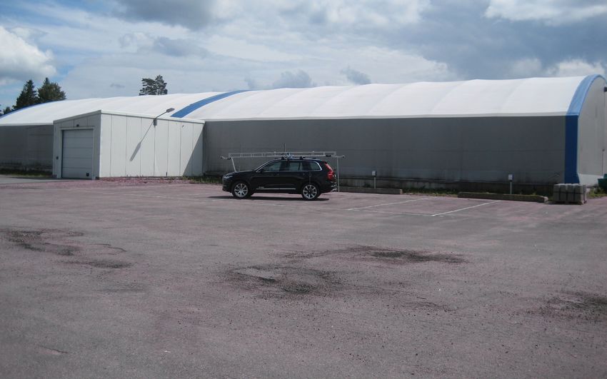
Targetless extrinsic calibration of vehicle-mounted lidars
CHRISTOFFER GILLBERG & KRISTIAN LARSSON

© CHRISTOFFER GILLBERG & KRISTIAN LARSSON, 2016.

Supervisors: Alex Rykov, Volvo Car Corporation & Dan Olsson, Infotiv AB
Examiner: Fredrik Kahl, Signals and Systems

Master’s Thesis 2016:EX097
Department of Signals and Systems
Image Analysis and Computer Vision Group
Chalmers University of Technology
SE-412 96 Gothenburg
Telephone +46 31 772 1000

Cover: Volvo XC90 with the reference system mounted on the roof, with the front,
left, and rear lidar visible in the photo.

Gothenburg, Sweden 2016

iv
Targetless extrinsic calibration of vehicle-mounted lidars
CHRISTOFFER GILLBERG & KRISTIAN LARSSON
Department of Signals and Systems
Chalmers University of Technology

Abstract
This thesis presents a method for unsupervised extrinsic calibration of multi-beam
lidars mounted on a mobile platform. The work was done on a reference sensing
system for low-speed manoeuvering, in development at Volvo Car Corporation. The
system is intended to create a detailed 3D representation of the immediate sur-
roundings of the vehicle. This representation will be used for performance analysis
of the vehicle’s on-board sensors, as well as provide ground truth for verification of
advanced driver assist functions.
    The calibration algorithm utilises lidar data recorded during vehicle movement,
combined with accurate positioning from a GPS/IMU, to map the surroundings.
Extrinsic calibration aims to find the mounting position and angle of the lidar,
and different values for the extrinsic calibration parameters will result in different
mappings. The assumption is made that the real world can be represented by a large
number of small continuous surfaces, and a mathematical description of how well
the mapping from a certain a set of calibration parameters fulfills this criterion is
introduced. This measure quantifies the distance from each measurement point to a
nearby surface constructed from its surrounding points, and the extrinsic calibration
is then found by optimising its value of this measure.
    The results show that this method can be used for extrinsic calibration of a single
lidar, with an accuracy that is beyond what is reasonable to expect from manual
measurements of the lidar position. The total remaining error after calibration was
2.9 cm and 0.85°, for translation and rotation respectively. The remaining error is
measured against the mean value for calibration done on 9 different data sets. This
shows both the superior accuracy of the method compare to manual measurements,
and the repeatability for different locations. The current implementation is a proof-
of-concept and as such has very long computation time, however several ways to
considerably shorten this time are suggested as future work. The presented method
has low operator dependency, and does not require any dedicated calibration targets.
This is a strength when data-collection and post-processing is done on different sites
and by different individuals. This method has potential to provide an easy-to-use
calibration procedure, that given a rough position estimate, can provide accurate
extrinsic calibration.

Keywords: extrinsic lidar calibration, multi-beam lidar, Velodyne VLP-16, point
cloud, reference sensor, verification

                                                                                     v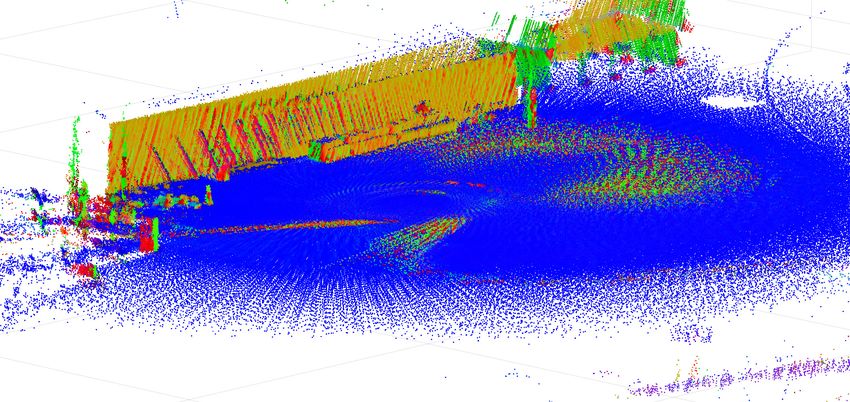
Acknowledgements
Throughout the thesis work many people have been helpful, and without this en-
gagement we would not have come this far. In general, we would like to thank several
engineers at Volvo Car Corporation (VCC) Active Safety department, as well as the
engineers at the VCC test facility Hällered Proving Ground.
    We would like to explicitly thank: Fredrik Kahl, for hours of supervising and
ideas that have been crucial for this thesis. Alex Rykov, for providing all necessary
equipment and for pushing the project at VCC and making this thesis possible.
Dan Olsson, for helping us in the thesis’ early phase. Teddy Hobeika, for letting us
borrow his high performance computer for extensive amount of computation (and
thus giving us a lot more results to present in this thesis). Edvin Pearsson, for
helping us with a lot of the practical work and being an all-round resource during
the late parts of the thesis.
    Finally a big thank you to our friends and family, who have put up with con-
tinuous talk of lidars for almost a year, and given us the support to finish this
thesis.

             Christoffer Gillberg & Kristian Larsson, Gothenburg, November 2016

                                                                                  vii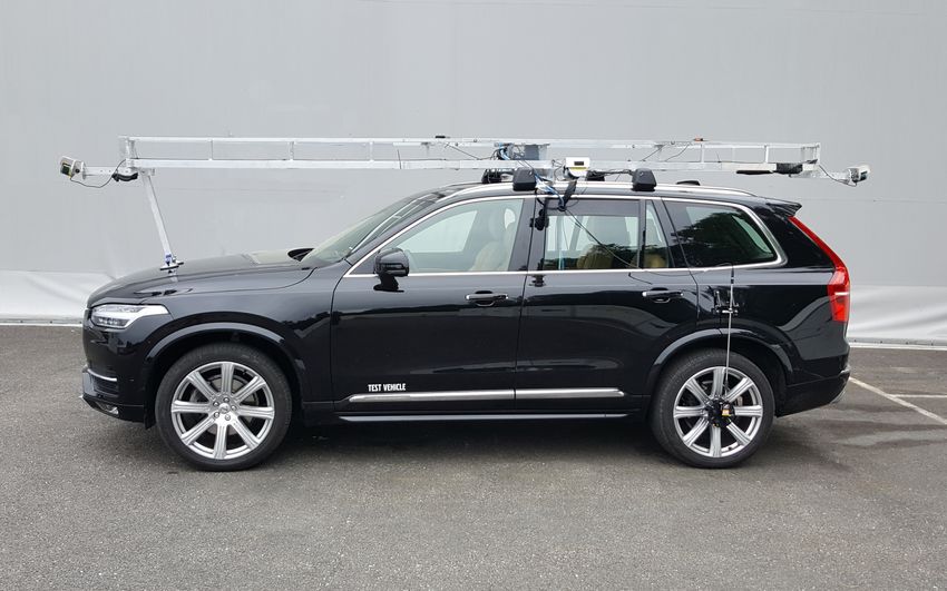
Contents

1 Introduction                                                                                                                       1
  1.1 Test and verification . . . . . . . . . . . .                     .   .   .   .   .   .   .   .   .   .   .   .   .   .   .    1
  1.2 What’s a lidar? . . . . . . . . . . . . . . .                     .   .   .   .   .   .   .   .   .   .   .   .   .   .   .    3
       1.2.1 Lidar mounting position calibration                        .   .   .   .   .   .   .   .   .   .   .   .   .   .   .    7
  1.3 Thesis aim . . . . . . . . . . . . . . . . . .                    .   .   .   .   .   .   .   .   .   .   .   .   .   .   .    9
       1.3.1 Limitations . . . . . . . . . . . . .                      .   .   .   .   .   .   .   .   .   .   .   .   .   .   .    9
       1.3.2 Calibration approaches . . . . . . .                       .   .   .   .   .   .   .   .   .   .   .   .   .   .   .    9

2 Hardware setup                                                                                                                    13
  2.1 Lidar - Velodyne VLP-16 .     .   .   .   .   .   .   .   .   .   .   .   .   .   .   .   .   .   .   .   .   .   .   .   .   13
  2.2 GPS/IMU - OxTS RT3003         .   .   .   .   .   .   .   .   .   .   .   .   .   .   .   .   .   .   .   .   .   .   .   .   15
      2.2.1 Wheel speed sensor      .   .   .   .   .   .   .   .   .   .   .   .   .   .   .   .   .   .   .   .   .   .   .   .   17
      2.2.2 GPS base station .      .   .   .   .   .   .   .   .   .   .   .   .   .   .   .   .   .   .   .   .   .   .   .   .   17

3 Background                                                                                                                        19
  3.1 Frames of reference . . . . . . . .           .   .   .   .   .   .   .   .   .   .   .   .   .   .   .   .   .   .   .   .   19
      3.1.1 Lidar frame: L . . . . . .              .   .   .   .   .   .   .   .   .   .   .   .   .   .   .   .   .   .   .   .   19
      3.1.2 Vehicle frame: V . . . . .              .   .   .   .   .   .   .   .   .   .   .   .   .   .   .   .   .   .   .   .   19
      3.1.3 Global frame: G . . . . .               .   .   .   .   .   .   .   .   .   .   .   .   .   .   .   .   .   .   .   .   20
  3.2 Coordinate transformations . . .              .   .   .   .   .   .   .   .   .   .   .   .   .   .   .   .   .   .   .   .   20
      3.2.1 Homogeneous coordinates                 .   .   .   .   .   .   .   .   .   .   .   .   .   .   .   .   .   .   .   .   21
      3.2.2 Transformation matrices .               .   .   .   .   .   .   .   .   .   .   .   .   .   .   .   .   .   .   .   .   21
  3.3 Synthetic lidar data . . . . . . . .          .   .   .   .   .   .   .   .   .   .   .   .   .   .   .   .   .   .   .   .   22

4 Calibration Method                                                                                                                25
  4.1 Single lidar extrinsic calibration . . . . . .                    .   .   .   .   .   .   .   .   .   .   .   .   .   .   .   25
      4.1.1 Objective function . . . . . . . . .                        .   .   .   .   .   .   .   .   .   .   .   .   .   .   .   27
      4.1.2 Modified objective function . . . .                         .   .   .   .   .   .   .   .   .   .   .   .   .   .   .   29
      4.1.3 Convexity of the objective function                         .   .   .   .   .   .   .   .   .   .   .   .   .   .   .   32
  4.2 Minimisation method . . . . . . . . . . . .                       .   .   .   .   .   .   .   .   .   .   .   .   .   .   .   34

5 Experimental procedure                                                         37
  5.1 Initial lidar position measurements . . . . . . . . . . . . . . . . . . . 37
  5.2 Sampling locations . . . . . . . . . . . . . . . . . . . . . . . . . . . . 38
  5.3 Issues with data acquisition and time stamps . . . . . . . . . . . . . . 39

6 Results                                                                                                                           43

                                                                                                                                    ix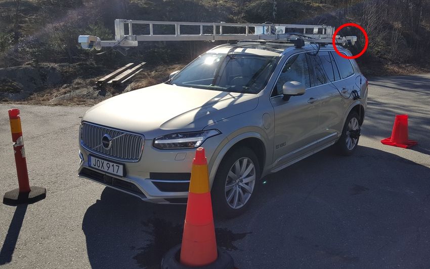
Contents

    6.1   Synthetic data . . . . . . . . . . .   .   .   .   .   .   .   .   .   .   .   .   .   .   .   .   .   .   .   .   .   43
          6.1.1 Convergence to true value        .   .   .   .   .   .   .   .   .   .   .   .   .   .   .   .   .   .   .   .   43
    6.2   Real data . . . . . . . . . . . . .    .   .   .   .   .   .   .   .   .   .   .   .   .   .   .   .   .   .   .   .   45
          6.2.1 Parameter selection . . . .      .   .   .   .   .   .   .   .   .   .   .   .   .   .   .   .   .   .   .   .   45
          6.2.2 Calibration results . . . .      .   .   .   .   .   .   .   .   .   .   .   .   .   .   .   .   .   .   .   .   47

7 Discussion                                                                                                                     55
  7.1 Calibration algorithm . . . . . . . . . . . . . . . . . . . . . . . . . . .                                                55
  7.2 Future work . . . . . . . . . . . . . . . . . . . . . . . . . . . . . . . .                                                56
  7.3 Conclusion . . . . . . . . . . . . . . . . . . . . . . . . . . . . . . . . .                                               58

Bibliography                                                                                                                     59

A Minimisation method                                                                                                              I

B Data sets                                                                                                                      III

C Calibration results                                                                                                             V

x
1
Introduction
Over the last decades, an increasing number of driver assistance functions have been
implemented in modern cars. An early example of a driver assistance function is
cruise control, which simply helps the driver to maintain a constant speed. With
more advanced and less costly sensors as well as faster processors, this technology
has become increasingly accessible and today the cruise control can be much more
complex where the car adapts the speed to its surroundings. More functions are
continuously implemented and the cars are becoming less dependent on the driver.
An important step in the development is verifying both sensor and function perfor-
mance. The verification is often done using a reference system including a 3D-laser
scanner (lidar). In this thesis a method of targetless and automatic calibration for
vehicle mounted lidars is presented.
Driver assistance functions such as adaptive cruise control are often referred as
Advanced Driver Assistance Systems, ADAS, and also include functions such as
driver drowsiness detection, lane departure warning/lane keeping aid and collision
avoidance. Another example of an ADAS function is semi-automatic parking, where
the car uses sensors to read the surroundings and control the steering to help the
driver park the car. However, the system is still dependent on the driver and can-
not park completely by itself, hence semi-automatic. The natural progression of
developing new driver assist functions is to create completely autonomous functions
which do not depend on the driver at all. Fully autonomous vehicles, or autonomous
driving, is currently a hot topic with major investments in research and develop-
ment. Many car manufacturers have announced that they will be testing prototype
autonomous cars on public roads within a few years [1]–[6].
The sensors needed for autonomous driving must work properly in all sorts of
traffic situations, in any weather and also both with and without daylight. The
system must therefore consist of a broad variety of different sensors such as sonars,
cameras and radars. The sensor data is then filtered or processed with various sensor
fusion methods in order to create a combined perception of the vehicle state and its
surroundings. With more sophisticated systems that control the vehicle, the need of
a high reliability is increased. The sensor readings need to be very accurate and the
system verification is an essential part of the development for autonomous drive.
1.1 Test and verification
To ensure that each of these ADAS or autonomous drive functions work properly, the
system needs to be verified. This can be done by performing a number of test cases,
11. Introduction
Figure 1.1: Field of view for the on-board sensors that sense the immediate vehicle
surroundings. These sensors are used in e.g. driver assistance functions such as
semi-automatic parking and collision warning [7].
designed to evaluate if any issues (or bugs) exist within the software or hardware.
With enough test cases it can with increasing certainty be said that the system is
verified to be working according to specification.
If the system is not tested thoroughly the output from the system can be very
different than what is intended. Fig. 1.1 shows the combined field of view for a
number of on-board sensors which are used to sense the immediate surroundings
of the vehicle. The data from these sensor can be used in for example collision
detection during automatic parking or other low-speed manoeuvres.
When verifying the on-board sensor systems used for ADAS and autonomous
drive, it is common to use some ground truth as reference. A ground truth is
considered to be the “true answer” of, in this case, the surroundings. It is used to
evaluate the performance of the vehicle’s own sensors in comparison to the ground
truth. Since the vehicle’s sensors’ data is the perception of the environment that the
ADAS functions then bases its decisions on, the performance of the sensors must
be known when determining the margin of error for the different functions. If the
sensor performance is worse then what the functions take into account, this can
lead to collisions during autonomous parking. Fig. 1.2 exemplifies why knowledge
of the sensor performance is important and what the difference can be compared to
the ground truth, by showing a collision that results from the sensors giving a very
different view then what the ground truth is. Once sensors performance is verified,
the ADAS functions themselves also must be verified to be safe and according to
specification. This in turn also requires a reference point, a ground truth, with
which to evaluate the method’s performance.
The ground truth can be obtained with many different methods of different
level of sophistication. For a case of verifying automatic parking of a car, one
straightforward way is to manually take relevant measurements using a tape ruler.
Relevant measurements could be the width of the parking spot, how well the car
places itself in it, and distance to adjacent objects and cars. This method is easily
available and useful for tests that are only done a few times. However if there are
hundreds, or even thousands, of different parking cases that need to be performed,
21. Introduction
Vehicle perception of its trajectory
True trajectory, “ground truth”
Figure 1.2: Vehicle sensor perception of the trajectory, compared to the ground
truth, i.e. the true trajectory, for a parking case.
and if each case requires manual measurements, this becomes very labour intensive.
In these cases a more automated method of obtaining the ground truth is preferred.
A ground truth for on-board sensor verification could then be a completely separate
reference system, consisting of sensor equipment with a higher precision then the
on-board sensors that are being verified.
1.2 What’s a lidar?
A possible solution for a reference system to the on-board sensors is to use lidar 1 .
The lidar technology is in essence a laser range meter (using time-of-flight range
measurement) where the beam is swept over the surroundings while continuously
taking range measurements. A simple lidar, shown in Fig. 1.3, can consist of only one
laser beam rotating a certain amount to map the surroundings. Current state-of-the-
art lidars consists of several beams, rotating 360° around a centre axis, measuring the
environment with high resolution and accuracy. These range measurements results
in data points of the surroundings, and put together they can shown a detailed
3-dimensional view of the world. The set of data points in a three dimensional
coordinate system is called a point cloud, which is the type of data obtained from a
lidar. An example of a small point cloud is shown in Fig. 1.4. This is the raw lidar
data for a single “frame”, or rotation, from a 64-beam lidar.
Lidar is commonly used in areas such as geo-mapping, with both airborne mea-
1
The word lidar is attributed two different origins: as an acronym of Light Detection And
Ranging (LIDAR), or as an portmanteau of light+radar=lidar [8]. There is no consensus on
capitalisation of the word, but the spelling using lower case is the most frequent in currently
available litterature [9]. The authors have chosen to use lower case for the word lidar throughout
this report.
31. Introduction Figure 1.3: Schematic image of the workings of a simple lidar. This example has a single beam reflected of a moveable mirror, letting the laser beam sweep 180° to perform range measurements, and thus map the surroundings. Figure 1.4: Typical 3D lidar raw data, created from a single rotation of a multi- beam lidar, mounted on the roof of a vehicle. In this case a 64-beam Velodyne HDL-64E [10]. 4
1. Introduction
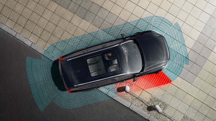
Figure 1.5: The test vehicle used in this thesis work. The reference system is built
by Volvo Car Corporation and used for verifying the vehicle’s on-board proximity
sensors. The proximity sensors’ field of view is shown in Fig. 1.1. The reference
system is mounted on top of the vehicle and includes four lidars, one placed on each
side of the car.
surements and on the ground, as well as a perception sensor for robotic applications.
Over the last decade, with a great leap after the DARPA Grand challenge in 2005
and 2007 [11], [12], the level of sophistication and accuracy of lidars have increased,
as well as reducing prices which has increased the accessibility of the technology.
This has made lidars popular as reference systems in the automotive industry and
they are now an important part of the sensor setup of autonomous vehicles. Because
of their high accuracy and detailed data, lidars are excellent to use as a ground truth
when verifying various functions on a vehicle. Volvo Car Corporation (VCC) has
developed a reference system to verify the vehicle’s proximity sensors, whose field of
view was shown in Fig. 1.1. The proximity sensors are used in different low-speed
manoeuvres, such as narrow lane keeping and automatic parking. The reference sys-
tem in development is shown in Fig. 1.5, and consists of four lidars, one on each side
of the vehicle. The system is intended to create an accurate view of the immediate
surroundings of the vehicle. This is the hardware system that was used throughout
the thesis.
By incrementally adding the new sensor data to a single point cloud (in a global
frame of reference) one can construct a map of the surroundings that the vehicle
moves through. This requires knowledge of the vehicle movement, and the sensor
position on the vehicle platform. Building a point cloud over time like this is called
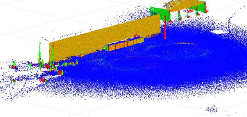
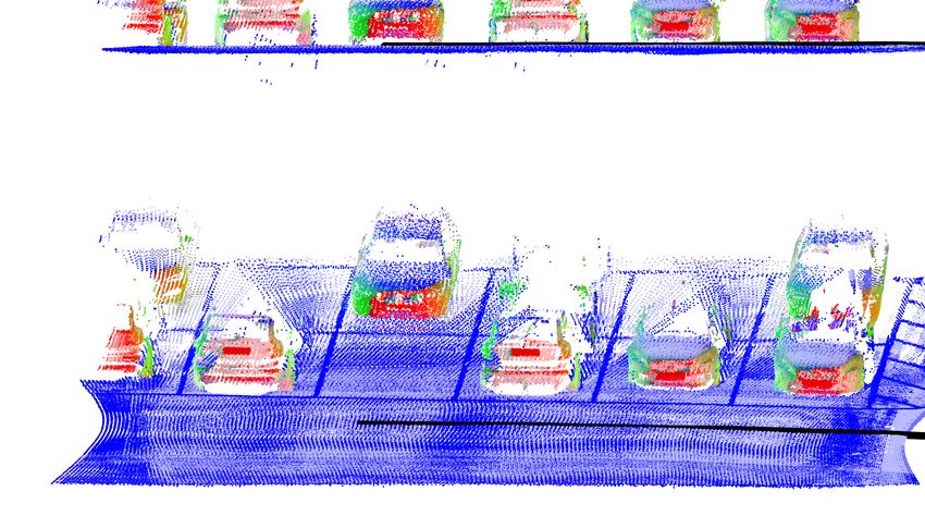
mapping. Fig. 1.6 shows an example of a map created from lidar data while driving
through a parking lot. Note that the lane markings are readily discernible when the
points are coloured based on reflection intensity.
The environment, or objects in it, is broadly classified as either being static or
dynamic. When sampling the environment, objects of two types are detected: either
objects which are stationary (static) during the entire sampling run, or objects which
are moving during the sampling run, called dynamic. Static objects includes the
51. Introduction Figure 1.6: Mapping of a parking lot, two rows with several cars parked, seen from two different angles. The black line indicates the trajectory of the vehicle’s rear-wheel axis (vehicle driven from right to left in the figure). Point cloud from 17 s of lidar data, 2.7·106 points, from the front mounted lidar as seen in Fig. 1.5. Points are coloured according to the surface normal vector at that point, with x, y, z components corresponding to red, green and blue channel, and colour saturation based on the intensity of the reflection for that point. ground, walls of buildings, parked cars, etc. Dynamic objects are typically other moving vehicles, bicyclists and pedestrians. When the sensor data is transformed to a global coordinate system, to create a single point cloud, all static objects will appear in the same location in the point cloud. Each point measured with the lidar will build a more dense point cloud reproduction of that object. Dynamic object on the other hand, have been moving during the sampling run, and when transformed into the global coordinate system they will appear in different locations of the point cloud. To successfully create a useful point cloud, points belonging to dynamic objects must be identified and cut away from the data when creating the map of the environment. When the dynamic objects are classified, useful information about them can be extracted, such as their size, position, velocity and heading. Separating static from dynamic objects is indeed possible, but requires sophisticated filtering methods for the data. The data from a lidar has a huge potential in what type of information can be extracted. By clustering (grouping points that likely belong to the same object) and segmentation (classifying points belonging to different regions), objects can be identified [13]. By further processing the object properties they can be classified to identify different types of objects. These classes could for example be static objects such as curb stones, lamp posts and walls, as well as dynamic objects such as other vehicles, mopeds, pedestrians and bicyclists. With this information at hand, combined with the distance and intensity data, the evaluation of the vehicle’s performance can be much more sophisticated. 6
1. Introduction

1.2.1     Lidar mounting position calibration
All the data processing to extract different information about the surrounding and
its objects is dependant on that the initial data is of high quality. One part in this
is of course using a high precision lidar, but another crucial part is knowing exactly
where in the vehicle coordinate system the lidar is mounted. Without this lidar
position, combining data recorded over time while the vehicle has moved will not
result in a useful mapped point cloud. The same can be said for combining data
from several lidars mounted differently: inaccurate calibration of the mounting po-
sition will result in two different sensors detecting e.g. the ground plane at different
heights or a pedestrian at two different positions. The extrinsic calibration, which
considers the mounting position of the entire lidar unit relative to the vehicle’s own
coordinate frame, needs to be accurate. If the setup must be able to measure dis-
tance from the vehicle to surrounding objects with for example 1 cm accuracy, the
mounting location of the lidar must known with a sub-centimetre accuracy. For the
angles of the mounting position this is doubly important. An error of just 1° in the
calibration translates to a measurement error of 17 cm for an object ten metres away.
Finding the lidar’s mounting location, the extrinsic calibration, is thus essential for
a reference system used as ground truth.
    The system used in this thesis is still in development and there is no procedure
for its extrinsic calibration. For a similar system that is already in use by VCC,
a reference system consisting of a single lidar, there is an established calibration
method. This method makes use of accurate manual measurements and which is
then used as an initial calibration guess. Data for a few seconds of sampling, while
the vehicle is moving, is then mapped on top of itself. For a correct calibration
the ground plane and any objects such as house walls will be contiguous surfaces.
However, for a poor calibration, the surfaces will not be properly aligned. The initial
calibration is then repeatedly adjusted manually until the surfaces appear to align,
by manual inspection. The level of accuracy needed for the calibration is dependant
on how the lidar data is going to be used. While the calibration is important for
a single lidar, it can still produce data of acceptable accuracy with a less accurate
calibration. If only a few seconds of data is mapped, any inaccuracies will not make
a drastic difference in the point cloud. For a system with multiple lidars, where the
data is intended to be combined together into a single point cloud, the accuracy
of calibration is more important. Combining a single 360° measurement from four
different lidars to a single coherent view of the surrounding, will not be possible if
they do not have a calibration of high accuracy. This effect is further amplified if
several seconds of data from each lidar is combined. For the lidar setup used in this
thesis, with four lidars, accurate calibration is therefore of high importance.
    In order to determine the lidar position a total of six parameters must be speci-
fied; the translation parameters x, y and z, and also three rotation parameters roll,
pitch, and yaw. Fig. 1.7b shows an example of the lidar coordinate frame with
respect to the vehicle coordinate frame.
    In addition to the extrinsic calibration, a lidar also has intrinsic parameters.
Lidars are manufactured to high accuracy and factory calibrated, in the sense that
all internal parameters that affect the reading are tuned to produce a reading that
is within some specification. However, with suitable methods the factory calibration

                                                                                      7
1. Introduction
L z
y
x
MV
z
V
z x y
y
G
x
(a) Frames of reference, showing the lidar frame L
for the left side lidar, the vehicle frame V and the
ground fix global frame G. The transformation MV
between V and L is indicated with a vector.
(b) The lidar system mounted on a vehicle. The
left side lidar is circled.
(c) Measurement data from a single rotation of
the left side lidar. Measured points (in blue) are
aligned and overlaid on the photograph of the ve-
hicle.
Figure 1.7: The car with the sensors mounted, and the three different frames of
reference G, V and L. The cones in the photograph are placed approximately in the
centre of the overlapping areas for the four lidars different field of view.
81. Introduction
can be further improvemed by finding the more precise parameter values for that
particular individual lidar. This is referred to as the intrinsic calibration. If the
manufacturer’s specifications of the lidar are acceptable, no intrinsic calibration
needs to be done. Some manner of extrinsic calibration, i.e. finding the mounting
position, must always be done if the data is going to be used in any other another
frame of reference than the lidar’s own.
1.3 Thesis aim
The aim of this thesis was to create a proof-of-concept for a lidar calibration method
for the reference sensing system built by Volvo Car Corporation. The reference sys-
tem is intended to create a detailed 3D representation of the immediate surroundings
of a vehicle. This means that the calibration of the system has to be accurate enough
so that the reference system can be used as a ground truth when verifying the accu-
racy of the vehicles on-board sensor systems and the performance of its autonomous
manoeuvres. The questions to answer with the thesis are firstly if the chosen method
of calibration works for this application, and secondly what accuracy can be achieved
and how it compares to what can be achieved by manual measurements.
1.3.1 Limitations
Each lidar is treated separately, as it would be the only lidar on the vehicle. The
fact that the reference system configuration has four lidars on the platform, with a
partially overlapping field of view, is not exploited in the calibration method. The
lidar measurements return both the measured point and the intensity of reflection
of that point. The data for intensity of the reflection is not used in the calibration
method.
This thesis will only consider extrinsic calibration. The intrinsic calibration is
deemed to be accurate enough already as specfied by the manufacturer, and these
specifications have also been verified in [14].
There are no requirements set on the computational speed on the calibration
method. This thesis will only focus on a proof-of-concept, leaving speed optimisation
as a future work. The calibration procedure is designed to run offline, i.e. during
post-processing of the data.
The calibration algorithm is not designed to handle dynamic objects, therefore
the data will need to be limited to static environments, or data where all dynamic
objects are removed. Filtering dynamic objects from the data is decided to be
outside the scope of the thesis. Therefore when doing sampling runs to collect lidar
data, it will be made sure that no moving objects are within detection range for the
lidar.
1.3.2 Calibration approaches
The first approach to extrinsic calibration is to by hand take measurements of the
lidar mounting position, using tape ruler and protractor. This has the benefit of
being easily accessible and straightforward, but the downside of large measurement
91. Introduction
errors and the result is user dependant. To reach the degree of accuracy needed for
a lidar system intended to be used as ground truth, more sophisticated automatic
methods must be employed.
There are several recently published works in the topic of extrinsic calibration
of lidars. Most methods are intended to be run offline, i.e. as post processing after
the data collection has been done. The computational intensity of the calibration
methods often prohibit them from being run online. An exception is Gao and
Spletzer [15], who suggests an online method where reflective markers are used as
calibration targets. This method is able to calibrate multiple lidars on the same
vehicle, however their conclusions state that further work on the accuracy is needed.
Maddern et al. have developed a method for unsupervised extrinsic lidar cal-
ibration, with positioning of the vehicle from a GPS/IMU, with good results in
accuracy [16]. The method of evaluating the point cloud quality is computationally
expensive, and they also presents faster, approximative, variants.
A supervised calibration method is suggested by Zhu and Liu [17] and provides
an improvement over factory calibration for the range measurement, however such
supervised calibration methods will be cumbersome for a setup with several lidars.
The calibration has the benefit of being straightforward and done by measuring
the distance to known obstacles in the environment, but as such it is very labour
intensive.
Brookshire and Teller presents a method of joint calibration for multiple coplanar
sensors on the same mobile vehicle [18]. Their method recovers the relative position
between two lidars, where the vehicle position itself is not known. This makes use
of the multiple lidars, which the system in this thesis have, however its intended use
is for smaller indoor vehicles, so it does not utilise the accurate positioning obtained
from the GPS/IMU.
A method capable extrinsic calibration of multiple 2D lidars is presented by He
et al. [19]. The method takes advantage of the overlapping fields of view from five
2D lidars, as well as positioning from GPS/IMU. They use classification of different
geometric features in the environment and matches the data from each lidar to
these features by adjusting the calibration. This method is promising for multi-lidar
setups, however it does not utilise the potential of 3D lidars, and in addition the
feature classification is done manually which does not make this a fully unsupervised
calibration method.
Levinson and Thrun has also conducted research in targetless extrinsic calibra-
tion of a 3D-lidar [20]. Their method recovers the calibration by alignment of sensed
three-dimensional surfaces. They formulate the calibration as a minimisation prob-
lem of the alignment of all surfaces in the sensed environment, where the minimal
solution is the correct calibration. In addition they shows that the same approach
can be used for calibration of intrinsic parameters. Their setup is similar to the one
in this thesis, with positioning from GPS/IMU and a Velodyne multi-beam lidar.
Some differences exists: the setup used in this thesis had a different lidar model,
which produced less dense data, as well as a different mounting angle of the lidar
compared to Levinson’s setup. It was decided this method was the most suitable
to be used for calibration of the reference system in this thesis. Partly because the
similarity of the setups, but also because of the relative simplicity of the implemen-
101. Introduction
tation and its future potential to use for intrinsic calibration as well as extrinsic.
As specified in the limitations of the thesis aim, no focus was put on computation
speed. The method presented in this thesis should theoretically be able to perform
similar to the implementation done by Levinson and Thrun in [20], whose calibration
procedure requires one hour of computation time on a regular laptop.
111. Introduction 12
2
                       Hardware setup

This section describes the different sensors used, how they are mounted and some
parts of the data acquisition. An schematic diagram of the system is shown in
Fig. 2.1 and, in essence, the setup consists of four lidars and one Inertial Mea-
surement Unit (IMU). Note that the GPS base station shown in the diagram is
technically not necessary for the system to work, however it greatly improves the
position accuracy and thereby also the accuracy of the results. The sensor placement
on the vehicle is shown in Fig. 2.2.
    All lidars were connected to a aluminium frame which in turn was mounted on
the roof rails on top of the vehicle. The frame is scalable, making it possible to
adjust the position of each lidar in both translation and rotation.
    The field of view for all four lidars is shown in Fig. 2.3. The field of view for
each lidar used in this thesis differs from the field of view in Fig. 1.4. This is due
to the fact that each lidar used in this thesis was mounted such that the centre axis
pointed almost horizontally, whereas the lidar used in Fig. 1.4 had its centre axis
pointed vertically. Each lidar therefore had a field of view on one side of the car
with some overlap at the corners. By adding the individual field of view from each
lidar, the system could map the area closest on all sides of the vehicle.

2.1     Lidar - Velodyne VLP-16
The specific lidars used during the thesis were four Velodyne VLP-16, shown in
Fig. 2.4a and with specifications in Tab. 2.1. This model has a small footprint
and a IP67 protection marking, making it suitable for automotive applications. It
is a multi-beam rotating lidar. The sensor has an array of 16 laser range finders
which rotates with 10 Hz around its centre axis while rapidly taking measurements,
approximately 300 000 measurements per second. The measurements are time of
flight distance measurement, and also returns the intensity of reflection.
    On a low level perspective, each measurement consists of a id number of the
beam, a rotation angle around the lidar’s axis, a distance and an intensity. However,
every measurement is transformed in the sensor software such that, for the end user,
each measurement simply consists of a point (xyz) in a Cartesian coordinate system,
where the lidar is located at the origin, seen by beam i and the intensity of the
reflection at that point.
    Each lidar is connected to a separate GPS unit, which is used to time stamp the
data. The time stamp is crucial when synchronising the lidar data to the others
sensors. The GPS time stamps for the lidars have a margin of error to the order of

                                                                                   13
2. Hardware setup
Lidar Lidar Lidar Lidar
GPS GPS GPS GPS
GPS
GPS
Antenna
IMU
DGPS
Logging computer
Wheel Speed Sensor
Figure 2.1: Connection diagram for the sensor setup used. The setup consisted of
four lidars with an individual GPS, as well as an GPS/IMU with several GPS’s and
a wheel speed sensor.
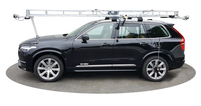
Figure 2.2: Mounting frame attached to vehicle, and with sensors circled. The
lidar on the passenger’s side is obscured in the figure but is mounted in the same
way as the lidar on the driver’s side, and the GPS/IMU is mounted inside the trunk
of the vehicle.
Figure 2.3: Placement indicated with red circles, and field of view for the four
lidars indicated in blue colour. Note that the lidars field of view have some overlap
at the corners of the car.
142. Hardware setup
CENTER AXIS
(MEASUREMENT ZERO)
(OPTICAL
CENTER)
2.00°
41.9mm
(a) Velodyne VLP-16 [21]. (b) Schematic figure with the beams shown.
The beams rotate around the centre axis dur-
ing measurement. Figure adopted from [22].
Figure 2.4: Velodyne VLP-16, the lidar model used during the thesis.
Table 2.1: Specifications for the accuracy of the VLP-16 lidar [22], [25].
Property Value and unit
Number of beams 16
Measurement range ≤100 m
Typical accuracy ± 3 cm
Rotation rate 5 − 20Hz
Field of view (vertical) 30◦ (+15◦ to −15◦ )
Beam separation (elevation angle) 2◦
Beam elevation angle accuracy ±0.11◦
Field of view (azimuth angle range) 0◦ − 360◦
Azimuth angle accuracy ±0.01◦
magnitude 10 ns [23]. This is accurate enough for this application, where a single
firing of each of the 16 lasers takes 55 µs [24].
Specifications for the VLP-16 is shown in Tab. 2.1. The angle between the beam
and the optical centre is called the elevation angle. The beam rotation around the
centre axis is denoted the azimuth angle. The measurement uncertainty presented
in the tabular is for the angles, however the data used is always transformed to
Cartesian coordinates. Because the measurement uncertainty is in both the range
reading and azimuth angle, the uncertainty is in fact dependant on what the range
to the object is from the sensor. A typical accuracy according to manufacturers
specification is ±3 cm. The validity of the manufacturers listed specifications of the
lidar was verified in [14], where the temperature stability was also tested and found
to be within acceptable bounds.
2.2 GPS/IMU - OxTS RT3003
The position of the vehicle is acquired from a so called GPS/IMU (Inertial Measure-
ment Unit). This is a single unit that has GPS coupled with IMU functions (gyro,
magnetometer and accelerometer), and uses Kalman filtering to estimate position,
152. Hardware setup
Figure 2.5: OxTS RT3003 from Oxford Technical Solutions, the GPS/IMU used
during the thesis [26].
Table 2.2: Specifications for the accuracy of the RT3003 Inertial Measurement
Unit [26].
Property Value and unit
Position (xyz) resolution (with RTK) ±0.01 m
Yaw angle (rz ) resolution ±0.1°
Pitch angle (ry ) resolution ±0.03°
Roll angle (rx ) resolution ±0.03°
velocity, acceleration and other states of the vehicle. The model used was an Ox-
ford Technical Solutions ‘RT3003v2’, shown in Fig. 2.5 [26]. During the thesis dual
GPS-antennas and a GPS base station were used with the RT3000, which allows the
position to be done using Real-Time Kinematic GPS (RTK GPS) [27]. This allows
for positioning accuracy of 1 cm. In addition to this a wheel speed sensor was also
used, which further improves the accuracy of the positioning by adding odometry
data. The RT3000-models have internal algorithms for finding its own mounting po-
sition in the vehicle reference frame given the proper initialisation procedure, which
lets the IMU produce data that is already in the vehicle’s frame (even if the IMU is
mounted with an offset to vehicle frame origin). Further accuracy specifications for
the RT3003 is listed in Tab. 2.2.
The position from the GPS/IMU is given as longitude[◦ ], latitude[◦ ] and alti-
tude[m]. To transform the point cloud the position must be in metres, however the
projection of spherical coordinates onto a flat surface will inevitably result in defor-
mations. To minimise the effect of such deformations, the coordinates are projected
according to the national map projection SWEREF 99 TM [28]. The largest defor-
mations are in longitudinal direction (east-west). Projection according to SWEREF
99 TM minimises these deformations by dividing Sweden into 12 different projection
zones, in effect 12 strips that share almost the same longitude. For data sampled at
Hällered Proving Ground, the projection zone 13°300 000 was used, and for Gothen-
burg, zone 12°00 000 .
162. Hardware setup
2.2.1 Wheel speed sensor
To improve the position accuracy from the IMU, a Wheel Speed Sensor (WSS) was
used. The sensor connects to one of the wheels, and measures the rotation with 8bit
accuracy, which means one wheel revolution is measured with a resolution of 1024
steps. The model used was a Pegasem Messtechnik GmbH “WSS3” [29].
2.2.2 GPS base station
To improve the GPS positioning accuracy, the option to use a ground fix GPS
base station was used. This required an additional radio receiver connected to the
IMU, as well as a GPS base station mounted within radio range (which typically
is several kilometres). This enables use of Differential GPS (DGPS), which means
that the base station records and transmits corrections to the current GPS position
indicated by the satellites. This can improve the position accuracy up to one order
of magnitude, from tens of centimetres to single digit centimetres [30]. For the
RT3003 the improvement was approximately from 20 cm with only GPS to 1 cm
with DGPS.
172. Hardware setup 18
3
                             Background

This chapter describes the notation used to formulate the calibration method math-
ematically, as well as some introduction to the synthetic lidar data which was used
through the thesis to verify the methods.

3.1      Frames of reference
In order to transform all lidar data into a single so called point cloud, three different
frames of referece has to be introduced; lidar frame, vehicle frame and global frame.
The different frames are described below.

3.1.1     Lidar frame: L
The data obtained from the lidar output is given as points in a Cartesian coordinate
frame with the lidar placed at the origin, as illustrated in Fig. 3.1. This frame
is called lidar frame, denoted L. Note that each lidar in the system has its own
coordinate frame, but since only one lidar at a time is calibrated the lidar frame
is always called L without distinguishing which one of the four lidars is currently
discussed.

3.1.2     Vehicle frame: V
The vehicle frame, denoted V , has the vehicle kept at the origin as shown in Fig. 3.2.
More precisely, the origin is placed at the centre of the rear wheel axis, but on ground
level.

Figure 3.1: Axis placement for the lidar frame. Aperture opening ω = ±15◦ and
azimuth angle α ∈ (0, 360)◦ [22].

                                                                                      19
3. Background
Figure 3.2: Frame of reference fixed to the vehicle, ISO8855 standard for road
vehicles [26]. This frame is referred as vehicle frame and denoted V in this thesis.
3.1.3 Global frame: G
The global frame, denoted G, is a ground fixed frame of reference where the origin
can be placed at an arbitrary local position on the ground. For practical reasons,
the origin is placed at the coordinates where the position measurement is initialised
for each individual data set.
3.2 Coordinate transformations
The measurement data in this thesis are all sampled in the lidar frame L, however
the calibration algorithm makes use of the data in the global frame G. The transfor-
mation between these two frames is a matter of simple coordinate transform, given
that the correct transformation matrices are known. The standard way of a rigid
transformation which includes both translation and rotation, is to first rotate and
then translate the point p in question as
p0 = R · p + t (3.1)
with R a rotation matrix, t a translation vector and p0 the transformed point.
The convention used for defining the rotation angles is yaw-pitch-roll, or (aero)nautical
angles [31]. The rotation matrix R is created by multiplying rotation around the
z, y, x-axis as follows:
R(rz , ry , rx ) = Rz (rz ) · Ry (ry ) · Rx (rx ), (3.2)
where the matrices for counter-clockwise rotation around the axis z, y, x with angles
rz , ry , rx are defined as:
cos(rz ) − sin(rz ) 0 cos(ry ) 0 sin(ry )
Rz (rz ) = sin(rz ) cos(rz ) 0 Ry (ry ) = 0 1 0
0 0 1 − sin(ry ) 0 cos(ry )
1 0 0
Rx (rx ) = 0 cos(rx ) − sin(rx )
. (3.3)
0 sin(rx ) cos(rx )
203. Background
The rotation is applied to a body-fix coordinate system. The first rotation is around
z-axis, then around the “new” rotated axis y 0 , and finally around the 2-times rotated
x00 axis. The rotation angles rz , ry , rx in this convention are referred to as yaw, pitch
and roll, respectively. This notation is used when referring to the pose of air crafts
or vehicles as the angle name relates directly to a specific movement. Note that the
sequence of rotations zyx around the body-fix frame is equivalent to a sequence of
rotations xyz around the current frame.
3.2.1 Homogeneous coordinates
If more then one transformation needs to be applied, the (3.1) way of writing quickly
becomes cumbersome. A convenient notation is then homogeneous coordinates [31].
Each measurement represents a point p = [x, y, z]T in space. In homogeneous coor-
dinates, the point is augmented as follows p̃ = [p; 1]. The transformation in (3.1) is
instead written as:
! !
0
R t p R·p+t
p̃ = M · p̃ = = . (3.4)
1 1
0 0 0 1
A single matrix multiplication p̃0 = M · p̃ can then apply both rotation and trans-
lation. A sequence of n coordinate transformations is expressed as:
p̃0 = M1 · M2 · ... · Mn · p̃. (3.5)
For simplicity the tilde notation for homogeneous coordinates is from here on disre-
garded. All point vectors p are assumed to be in homogeneous coordinates.
3.2.2 Transformation matrices
For this thesis two coordinate transformations are particularly interesting: from
global frame G to vehicle frame V , and from vehicle frame V to lidar frame L.
These are denoted:
• MV = MV (xcal ): Lidar frame to vehicle frame. The lidars are assumed to
rigidly attached to the vehicle, so this transformation is an (unknown) constant
matrix. The position of the lidar has both translation and rotation with respect
to the vehicle frame. These six parameters are called the calibration vector
xcal = [x, y, z, rx , ry , rz ].
• MG = MG (t) = MG (xvehicle (t)): Vehicle frame to global frame. This is the pose
of the ego vehicle, with six degrees of freedom. The pose varies with time, and
is measured using the IMU. The individual position parameters for the vehicle
xvehicle (t) = [x(t), y(t), z(t), rx (t), ry (t), rz (t)] are never explicitly used outside
of the implementation in code, so MV (t) is written as just dependant on time
t, to keep the notation shorter.
213. Background
Measured data points from the lidar are written as
(frame)
p(measurement index) . (3.6)
The k:th measurement point, projected in the lidar’s own frame L, is written as pLk .
Transformed to vehicle frame it is
pVk (xcal , tk ) = MV (xcal ) · pLk (tk ) (3.7)
and transformed to global frame
pG L
k = MG (tk ) · MV (xcal ) · pk (tk ) (3.8)
| {z }
=pV
k
(xcal ,tk )
where tk is the sampling time for point pk . As stated previously, MG (tk ) is created
from the vehicle pose, and since the vehicle is moving, it is dependant on time.
To transform a single point pLk (tk ) from lidar frame to global frame, the vehicle
pose at the time of sampling for that point must be used to create MG (tk ). When
transforming an entire sampling run consisting of several million data points, MG is
different for each point, while MV is constant since lidar mounting position on the
vehicle remains constant.
3.3 Synthetic lidar data
The development of the calibration algorithm required some realistic data in order
to test the functionality of the code. While real data was accessible, any problems
that would emerge in the computations could be either due to issues with the data,
problems with the algorithm itself or from the search method used. A way to have
control over all the sensors, sources of noise, and world parameters, is to use data
generated from a simulated environment. The true calibration values, i.e. the sensor
position xcal , can also never be known for the real system, while they are trivially
known from synthetic data where the user configures everything.
The simulation environment was constructed to work in principle like the real
physical system does, i.e. a mobile vehicle with a number of sensors that is traversing
some world. The simulated world is represented by a number of polygons represent-
ing ground plane, buildings and other vehicles. The sensor is represented by a large
number of rays emitted from the same point. The vehicle is simply a coordinate
and the sensor is attached a fixed distance from the vehicle origin. During a simu-
lation run the vehicle is moved through a series of positions. For each position in
the trajectory, the intersection between the sensor rays and the world polygons is
computed. These intersections represent where the lidar’s lasers would have hit the
real world object, causing a detection. A simulation run where the vehicle moves
to three different poses, and has a single front mounted lidar, is shown in Fig. 3.3.
The coloured dots are the intersections between the laser beams and the grey world
objects. Note that each “firing” of the lidar results in a thin strip of detections
across the simulation world. An example of a simulation run which is closer to the
type of data the real system will produce, is shown in Fig. 3.4.
223. Background
Figure 3.3: Simulated sampling run consisting of three vehicle poses. The simu-
lation world consists of grey polygons representing ground and buildings. The lidar
measurements from the three poses are also plotted, with one colour for each vehicle
pose.
Figure 3.4: Example of a synthetic data set with coloured lidar detection points.
The surrounding is the same as in Fig. 3.3 but from a different view. The black line
represents the trajectory of the vehicle, driving in a figure-eight through roughly
500 different poses. The point cloud is coloured according to each point’s surface
normal, with xyz component controlling the red, green and blue colour.
233. Background
The data is created in the global frame G. To use it to test the calibration
algorithm, the synthetic lidar data is transformed to lidar frame L. Based on (3.8)
and multiplying with the inverse transformations of the true calibration
−1 −1
pLk (tk ) = MV (xtrue ) · MG (tk ) · pG
k. (3.9)
A synthetic data set consists of the set of points pLk sorted based on what lidar
beam they were sampled with, and the set of vehicle poses MG (t) for the entire
simulation run. The data sets emulates using ideal, noiseless, sensors. When noisy
data was wanted, the noise was set as a normal distributed deviation from the true
sensor measurements. As listed in Sec. 2.1 the sensors have a typical deviation of
3 cm for the measurement. The noise in the real lidar is caused by uncertainty
in azimuth angle, elevation angle and range measurement. This means that the
uncertainty in measurement depends on the distance, and the elevation angle is
a fix angle (but its true value is not know). Therefore the sensor noise on the
measurements xyz is not expected to be completely normal distributed. However as
a simplification the noise for the synthetic data is created as a normal distributed
error from the noise-free lidar measurements of xyz. This simplification could be
done since the robustness to the real noise would be tested when using the real data
sets anyway.
244
Calibration Method
This chapter describes the method used for the extrinsic calibration. As mentioned
in Sec. 3.2, extrinsic calibration is equivalent of finding the transformation matrix
MV . This transformation is used when transforming a point pL (lidar frame) to
pG (global frame). Because the point cloud data is recorded while the vehicle is
moving, each lidar measurement will be taken from a slightly different pose of the
vehicle. Transforming the recorded point cloud from the lidar frame to the global
frame includes this time dependent transformation as well as MV as follows:
pG = MG (t) · MV (x) · pL (t), (4.1)
where MG (tp ) is the transformation from vehicle to global frame at time t, created
with IMU information. MV (x) is the transformation matrix based on a calibration
vector x.
Changing the calibration vector x results in an complex transformation of the
entire point cloud. Therefore traditional methods of point cloud registration such as
Iterative Closest Point (ICP) [32] cannot be used, as ICP assumes the entire point
cloud needs to undergo the same transformation. The calibration algorithm used in
this thesis is based on work done by Levinson and Thrun in [20]. They present a
method for extrinsic calibration of a multi-beam 3D-lidar mounted on a vehicle. It
is similar to ICP and point-to-plane matching, but with some differences specific to
this type of registration (or calibration) problem. Their algorithm makes use of both
the properties of a multi-beam lidar as well as the fact that the system is mounted
on a mobile platform. The first section below explains the calibration method as
introduced by Levinson/Thrun and following that the modifications done for the
implementation used in this thesis are presented.
The proof-of-concept for the calibration method in this thesis was done in Mat-
lab [33], using its implementation of nearest neighbour search from [34] and surface
normal methods included in the Computer Vision System-toolbox. Matlab was
chosen for its ease of implementation and testing of ideas, and since no strict re-
quirement on computation time was set, Matlab’s slower computation speed was
acceptable.
4.1 Single lidar extrinsic calibration
The calibration method in [20] was developed with the Velodyne HDL-64E [35] in
mind, a lidar similar to VLP-16 but with 64 beams instead of 16. The method makes
use of the fact that the lidar has several beams, with fix angles between them, which
254. Calibration Method
can map the entire surrounding. In addition to the lidar data, the algorithm also
needs accurate vehicle pose in some ground-fix frame of reference. This frame may
be local to the sampling site, rather than absolute longitude, latitude, and altitude
coordinates. What is important is to obtain the movement and heading of the vehicle
relative to the static environment, during a sampling run. Similar to the setup for
this thesis, Levinson/Thrun uses a GPS/IMU to obtain position data.
The rotating multi-beam lidars return huge amounts of measurement data which
opens up for new approaches to calibration. Combined with the vehicle pose data,
and knowledge of where and how the lidar is placed on the vehicle, the lidar data
can be transformed to a dense point cloud representation of the surrounding en-
vironment. An observation is made that the world tends to consist of contiguous
surfaces - in contrary to random points scattered in the air. The calibration method
is based on the idea that the best calibration will be one for which the world de-
scribed by the point cloud is as close as possible to a world represented by small
plane surfaces. By testing different transformations and evaluating how well the
tested transformation fulfils this criterion, the true calibration values can be found,
or closely approximated.
The algorithm uses the assumption that the surrounding environment is static.
This is important since the lidar samples data over time which then transforms
every point into a single global and time independent point cloud. Dynamic objects,
objects which move during the sampling run, will result in a more noisy mapping of
the environment.
Apart from a static environment, the algorithm also uses the assumption that the
environment can be represented as small and smooth surfaces. This assumption is
typically true when measuring urban environments consisting mostly of flat ground,
buildings and other vehicles. This assumption does not hold when measuring in less
structured environments such as parks, since grass and trees are not locally smooth.
However, an urban environment with a few trees or other non-smooth object is not
an issue, as long as these objects only make up a smaller portion of the point cloud.
Using these assumptions, a way to measure how well a certain transformation
from lidar to vehicle frame conform to the true transformation, is to compute how
close all the points in the point cloud are to small surfaces constructed from their
closest neighbouring points. In general, one can calculate the distance d from a
point to a plane by
d = kη · (p − m)k (4.2)
where p is the point of interest, η surface normal to a plane and m is a point on that
plane. The distance d between the point pk and the plane around mk is illustrated
in Fig. 4.1.
If d is computed for all the points in the point cloud, and a calibration xcal where
the sum of all distances d is as low as possible is somehow found, xcal should be the
true calibration. To further supress points far from surfaces, the distance is squared
before summation. This results in that single large deviations from the plane is
supressed while many small deviations are accepted, which is the wanted behaviour.
264. Calibration Method
z pk
d
y
ηk mk
x
Figure 4.1: Small point cloud (the circles) with a plane ηk fitted to the nearest
neighbours of mk . The point closest to mk is pk . The perpendicular distance
between the fitted plane and pk , is indicated as d.
Summation of all values d:
kηk · (pk − mk )k2 .
X
Dsum = (4.3)
k
The minimum of Dsum is found when the true calibration vector x∗cal is used to
transform the point cloud. For a synthetic data set without noise, the value of Dsum
is close to zero. Fig. 4.2 shows two examples of a synthetic dataset transformed
to the global frame using the true calibration, and a calibration which deviates 20°
from the true value around the x-axis. Note that the erroneous calibration results
in a point cloud where the surfaces are distorted. A 20° error in calibration is highly
exaggerated but the effect is the same even for small deviations from the true value.
4.1.1 Objective function
Levinson/Thrun introduces an objective function, based on the idea of Dsum from
equation (4.3), which penalises the points which lies far away from planes defined
by its neighbouring points. The lidar that is being calibrated with this method has
B individual laser beams with which measurements are made. The beams have a fix
elevation angle relative to the optical centre (seen in Fig. 2.4b). The measurement
and calibration of this angle belongs to the intrinsic calibration. To reduce the
impact that any errors in the calibration of the elevation angle has on the extrinsic
calibration method, the point cloud data is separated per beam. A plane fitted to
data from all beams will have the different errors in elevation angle from all beams
affect the orientation of the plane, while the orientation of a plane fitted to data
points from a single beam will not be effected in the same way, since the error in
alignment of the created plane will only come from the error of a single beam, and
not from all beams. Creation of the plane is illustrated in Fig. 4.1.
The lidar data is sorted based on what beam the data was sampled with. A
full data set D = B
S
i=1 P(i) from a lidar consists of B number of subsets of data
points from each of the lidar’s beams. The algorithm loops over these data sets
when calculating the value of the objective function.
27You can also read