Four decades of Antarctic surface elevation changes from multi-mission satellite altimetry
←
→
Page content transcription
If your browser does not render page correctly, please read the page content below
The Cryosphere, 13, 427–449, 2019
https://doi.org/10.5194/tc-13-427-2019
© Author(s) 2019. This work is distributed under
the Creative Commons Attribution 4.0 License.
Four decades of Antarctic surface elevation changes from
multi-mission satellite altimetry
Ludwig Schröder1,2 , Martin Horwath1 , Reinhard Dietrich1 , Veit Helm2 , Michiel R. van den Broeke3 , and
Stefan R. M. Ligtenberg3
1 Technische Universität Dresden, Institut für Planetare Geodäsie, Dresden, Germany
2 Alfred Wegener Institute, Helmholtz Centre for Polar and Marine Research, Bremerhaven, Germany
3 Institute for Marine and Atmospheric Research Utrecht, Utrecht University, Utrecht, the Netherlands
Correspondence: Ludwig Schröder (ludwig.schroeder@tu-dresden.de)
Received: 6 March 2018 – Discussion started: 19 March 2018
Revised: 13 January 2019 – Accepted: 16 January 2019 – Published: 5 February 2019
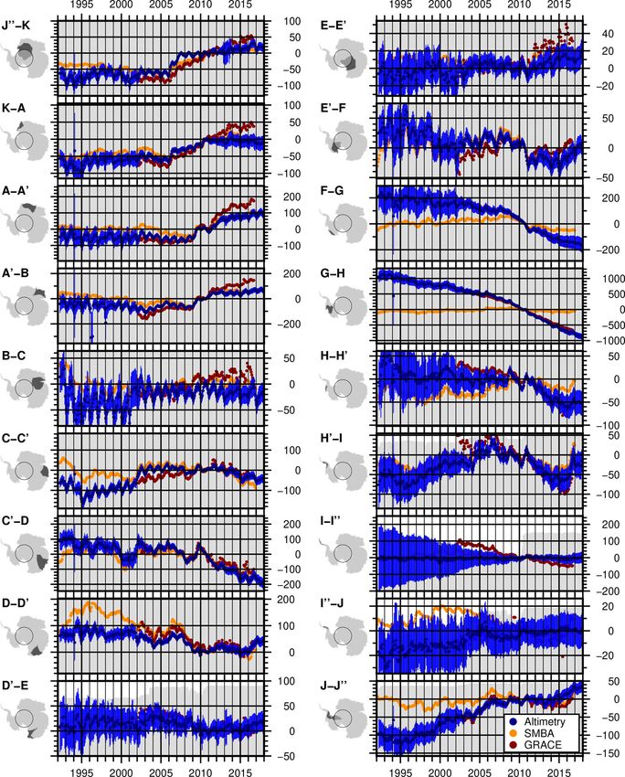
Abstract. We developed a multi-mission satellite altime- 1 Introduction
try analysis over the Antarctic Ice Sheet which comprises
Seasat, Geosat, ERS-1, ERS-2, Envisat, ICESat and CryoSat- Satellite altimetry is fundamental for detecting and under-
2. After a consistent reprocessing and a stepwise calibration standing changes in the Antarctic Ice Sheet (AIS; Rémy and
of the inter-mission offsets, we obtained monthly grids of Parouty, 2009; Shepherd et al., 2018). Since 1992, altime-
multi-mission surface elevation change (SEC) with respect ter missions have revealed dynamic thinning of several out-
to the reference epoch 09/2010 (in the format of month/year) let glaciers of the West Antarctica Ice Sheet (WAIS) and have
from 1978 to 2017. A validation with independent elevation put narrow limits on elevation changes in most parts of East
changes from in situ and airborne observations as well as a Antarctica. Rates of surface elevation change are not con-
comparison with a firn model proves that the different mis- stant in time (Shepherd et al., 2012). Ice flow acceleration
sions and observation modes have been successfully com- has caused dynamic thinning to accelerate (Mouginot et al.,
bined to a seamless multi-mission time series. For coastal 2014; Hogg et al., 2017). Variations in surface mass bal-
East Antarctica, even Seasat and Geosat provide reliable in- ance (SMB) and firn compaction rate also cause interannual
formation and, hence, allow for the analysis of four decades variations of surface elevation (Horwath et al., 2012; Shep-
of elevation changes. The spatial and temporal resolution of herd et al., 2012; Lenaerts et al., 2013). Consequently, differ-
our result allows for the identification of when and where sig- ent rates of change have been reported from altimeter mis-
nificant changes in elevation occurred. These time series add sions that cover different time intervals. For example, ERS-1
detailed information to the evolution of surface elevation in and ERS-2 data over the interval 1992–2003 revealed nega-
such key regions as Pine Island Glacier, Totten Glacier, Dron- tive elevation rates in eastern Dronning Maud Land and En-
ning Maud Land or Lake Vostok. After applying a density derby Land (25–60◦ E) and positive rates in Princess Eliza-
mask, we calculated time series of mass changes and found beth Land (70–100◦ E) (Wingham et al., 2006b), while En-
that the Antarctic Ice Sheet north of 81.5◦ S was losing mass visat data over the interval 2003–2010 revealed the oppo-
at an average rate of −85 ± 16 Gt yr−1 between 1992 and site pattern (Flament and Rémy, 2012). Two large snowfall
2017, which accelerated to −137 ± 25 Gt yr−1 after 2010. events in 2009 and 2011 induced stepwise elevation changes
in Dronning Maud Land (Lenaerts et al., 2013; Shepherd
et al., 2012).
As a consequence, mean linear rates derived from a single
mission have limited significance in characterizing the long-
term evolution of the ice sheet (Wouters et al., 2013). Data
from different altimeter missions need to be linked over a
time span that is as long as possible in order to better distin-
Published by Copernicus Publications on behalf of the European Geosciences Union.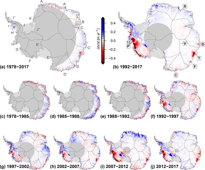
428                                                               L. Schröder et al.: Multi-mission altimetry in Antarctica

guish and understand the long-term evolution and the natural      with the extended time series from satellite altimetry. Finally,
variability of ice sheet volume and mass.                         we calculate ice sheet mass balances from these data for the
   Missions with similar sensor characteristics have been         covered regions. A comparison with independent data indi-
combined, e.g., by Wingham et al. (2006b, ERS-1 and               cates a high consistency of the different data sets but also
ERS-2) and Li and Davis (2008, ERS-2 and Envisat).                reveals remaining discrepancies.
Fricker and Padman (2012) use Seasat, ERS-1, ERS-2 and
Envisat to determine elevation changes of Antarctic ice
shelves. They apply constant biases, determined over open         2     Data
ocean, to cross-calibrate the missions. In contrast to ocean-
                                                                  2.1    Altimetry data
based calibration, Zwally et al. (2005) found significant dif-
ferences for the biases over ice sheets with a distinct spa-      We use the ice sheet surface elevation observations from
tial pattern (see also Frappart et al., 2016). Khvorostovsky      seven satellite altimetry missions: Seasat, Geosat, ERS-1,
(2012) showed that the correction of inter-mission offsets        ERS-2, Envisat, ICESat and CryoSat-2. Figure 1 gives an
over an ice sheet is not trivial. Paolo et al. (2016) cross-      overview of their temporal and spatial coverage. The data
calibrated ERS-1, ERS-2 and Envisat on each grid cell using       of the two early missions, Seasat and Geosat, were obtained
overlapping epochs, and Adusumilli et al. (2018) extended         from the Radar Ice Altimetry project at Goddard Space Flight
these time series by including CryoSat-2 data. We use a very      Center (GSFC). For the ESA missions, we used the data of
similar approach for conventional radar altimeter measure-        the REAPER reprocessing project (Brockley et al., 2017) of
ments with overlapping mission periods. Moreover, we also         ERS-1 and ERS-2, the RA-2 Sensor and Geophysical Data
include measurements of the nonoverlapping missions Seasat        Record (SGDR) of Envisat in version 2.1 and Baseline C
and Geosat and measurements with different sensor charac-         Level 2I data of CryoSat-2. For ICESat we used GLA12
teristics, such as ICESat laser altimetry or CryoSat-2 inter-     of release 633 from the National Snow and Ice Data Cen-
ferometric synthetic aperture radar (SARIn) mode, making          ter (NSIDC). Further details concerning the data set versions
the combination of the observations even more challenging.        used and the data-editing criteria applied to remove corrupted
   Here we present an approach for combining seven differ-        measurements in a preprocessing step are given in the Sup-
ent satellite altimetry missions over the AIS. Using refined      plement.
waveform retracking and slope correction of the radar altime-        As illustrated in Fig. 1, due to the inclination of 108◦ ,
try (RA) data, we ensure the consistency of the surface ele-      Seasat and Geosat measurements only cover the coastal re-
vation measurements and improve their precision by up to          gions of the East Antarctic Ice Sheet (EAIS) and the north-
50 %. In the following stepwise procedure, we first process       ern tip of the Antarctic Peninsula Ice Sheet (APIS) north of
the measurements from all missions jointly using the repeat-      72◦ S, which is about 25 % of the total ice sheet area. With the
altimetry method. We then form monthly time series for each       launch of ERS-1, the polar gap was reduced to areas south of
individual mission data set. Finally, we merge all time series    81.5◦ S, resulting in coverage of 79 % of the area. The polar
from both radar and laser altimetry. For this last step, we em-   gap is even smaller for ICESat (86◦ S) and CryoSat-2 (88◦ S),
ploy different approaches of inter-mission offset estimation,     leading to a nearly complete coverage of the AIS in recent
depending on the temporal overlap or nonoverlap of the mis-       epochs.
sions and on the similarity or dissimilarity of their altimeter      ERS-1 and ERS-2 measurements were performed in two
sensors.                                                          different modes, distinguished by the width of the tracking
   We arrive at consistent and seamless time series of grid-      time window and the corresponding temporal resolution of
ded surface elevation differences with respect to a refer-        the recorded waveform. The ice mode is coarser than the
ence epoch (09/2010; in the format of month/year) which we        ocean mode, in order to increase the chance of capturing the
made publicly available at https://doi.pangaea.de/10.1594/        radar return from rough topographic surfaces (Scott et al.,
PANGAEA.897390 (Schröder et al., 2019). The resulting             1994). While the ice mode was employed for the major-
monthly grids with a 10 km spatial resolution were obtained       ity of measurements, a significant number of observations
by smoothing with a moving window over 3 months and a             have also been performed in the ocean mode over Antarctica
spatial Gaussian weighting with 2σ = 20 km. We evaluate           (22 % for ERS-1, 2 % for ERS-2). We use the data from both
our results and their estimated uncertainties by a compari-       modes, as the ocean mode provides a higher precision while
son with independent in situ and airborne data sets, satellite    the ice mode is more reliable in steep terrain (see Figs. S1
gravimetry estimates and regional climate model outputs. We       and S3 in the Supplement). However, as there is a region-
illustrate that these time series of surface elevation change     ally varying bias between the modes, we treat them as two
(SEC) allow for the study of geometry changes and derived         separate data sets, similar to Paolo et al. (2016).
mass changes of the AIS in unprecedented detail. The re-
cent elevation changes of Pine Island Glacier in West Antarc-
tica, Totten Glacier in East Antarctica and Shirase Glacier of
Dronning Maud Land in East Antarctica are put in context

The Cryosphere, 13, 427–449, 2019                                                      www.the-cryosphere.net/13/427/2019/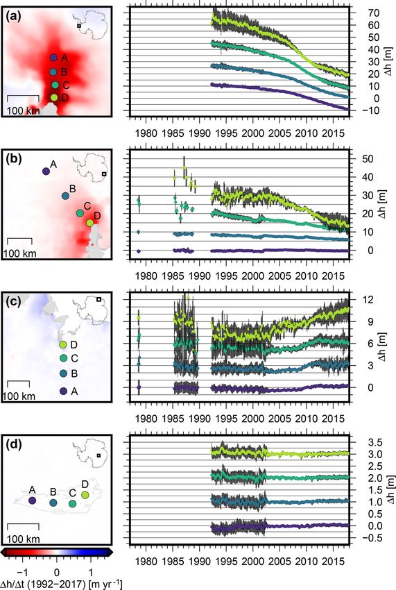
L. Schröder et al.: Multi-mission altimetry in Antarctica                                                                              429

Figure 1. Spatial and temporal coverage of the satellite altimetry data used in this study. The colors denote the maximum southern extent of
the measurements (dark blue: 72◦ S, light blue: 81.5◦ S, orange: 86◦ S, red: 88◦ S) and thus the size of the respective polar gap.

2.2   Reprocessing of radar altimetry                                   tion. In order to achieve a subgrid POCA location, we fit a bi-
                                                                        quadratic function to the satellite-to-surface distance within
Compared to measurements over the global oceans, pulse-                 a 3 × 3 grid cell environment around the coarse POCA grid
limited radar altimetry (PLRA) over ice sheets requires a spe-          cell and determine the POCA according to this function.
cific processing to account for the effects of topography and              The retracking of the return signal waveform is another
the dielectric properties of the surface (Bamber, 1994). To             important component in the processing of RA data over ice
ensure consistency in the analysis of PLRA measurements,                sheets (Bamber, 1994). Functional fit approaches (e.g., Mar-
processed and provided by different institutions, we applied            tin et al., 1983; Davis, 1992; Legrésy et al., 2005; Wingham
our own method for retracking and slope correction.                     et al., 2006b) are well established and allow the interpre-
    The slope correction is applied to account for the effect of        tation of the obtained waveform shape parameters with re-
topography within the beam-limited footprint (Brenner et al.,           spect to surface and subsurface characteristics (e.g., Lacroix
1983). Different approaches exist to apply a correction (Bam-           et al., 2008; Nilsson et al., 2015). However, the alternative
ber, 1994), but this effect is still a main source of error in RA       approach of threshold retrackers has proven to be more pre-
over ice sheets. The “direct method” uses the surface slope             cise in terms of repeatability (Davis, 1997; Nilsson et al.,
within the beam-limited footprint to obtain a correction for            2016; Schröder et al., 2017). A very robust variant is called
the measurement in the nadir direction. In contrast, the “re-           ICE-1, using the “offset center of gravity” (OCOG) ampli-
location method” relates the measurement towards the likely             tude (Wingham et al., 1986). Compared to the waveform
true position up slope. While the direct method has the ad-             maximum, the OCOG amplitude is significantly less affected
vantage that the measurement location is unchanged, which               by noise (Bamber, 1994). Davis (1997) compared different
allows an easier calculation of profile crossovers or repeat-           retrackers and showed that a threshold-based retracker pro-
track parameters, the relocation method has lower intrinsic             duces remarkably higher-precision results (especially with a
error (Bamber, 1994). A validation using crossovers with                low threshold as 10 %), compared to functional-fit-based re-
kinematic GNSS-profiles (Schröder et al., 2017) showed that,            sults. We implemented three threshold levels (10 %, 20 % and
especially in coastal regions, the direct method leads to sig-          50 %) for the OCOG amplitude, which allowed us to ana-
nificantly larger offsets and standard deviations, compared             lyze the influence of the choice of this level, similar to Davis
to the relocation method. Roemer et al. (2007) developed a              (1997).
refined version of the relocation method, using the full in-               In addition to PLRA, we also use the SARIn mode data of
formation of a digital elevation model (DEM) to locate the              CryoSat-2, reprocessed by Helm et al. (2014). The difference
point of closest approach (POCA) within the approximately               with respect to the processing by ESA mainly consisted of a
20 km beam-limited footprint. We applied this method in our             refined determination of the interferometric phase and of the
reprocessing chain using the DEM of Helm et al. (2014).                 application of a threshold retracker.
The CryoSat-2 measurements, used for this DEM, have very
dense coverage, and hence very little interpolation is neces-           2.3    Accuracy and precision
sary. Compared to the DEM of Bamber et al. (2009), this
significantly improves the spatial consistency. We optimized            The accuracy of RA-derived ice surface elevation measure-
the approach of Roemer et al. (2007) with respect to com-               ments has been assessed previously by a crossover compar-
putational efficiency for application over the entire ice sheet.        ison with independent validation data such as the ICESat
Instead of searching the POCA with the help of a moving                 laser observations (Brenner et al., 2007), airborne lidar (Nils-
window of 2 km (which represents the pulse-limited foot-                son et al., 2016) and ground-based GNSS profiles (Schröder
print) in the DEM-to-satellite grid, we applied a Gaussian              et al., 2017). Besides the offset due to snowpack penetration
filter with σ = 1 km to the DEM itself to resemble the cover-           and instrumental calibration over flat terrain, these assess-
age of a pulse-limited footprint. Hence, instead of the closest         ments revealed that, with increasingly rough surface topog-
window average, we can simply search for the closest cell in            raphy, the RA measurements show systematically higher el-
the smoothed grid, which we use as the coarse POCA loca-                evations than the validation data. These topography-related

www.the-cryosphere.net/13/427/2019/                                                               The Cryosphere, 13, 427–449, 2019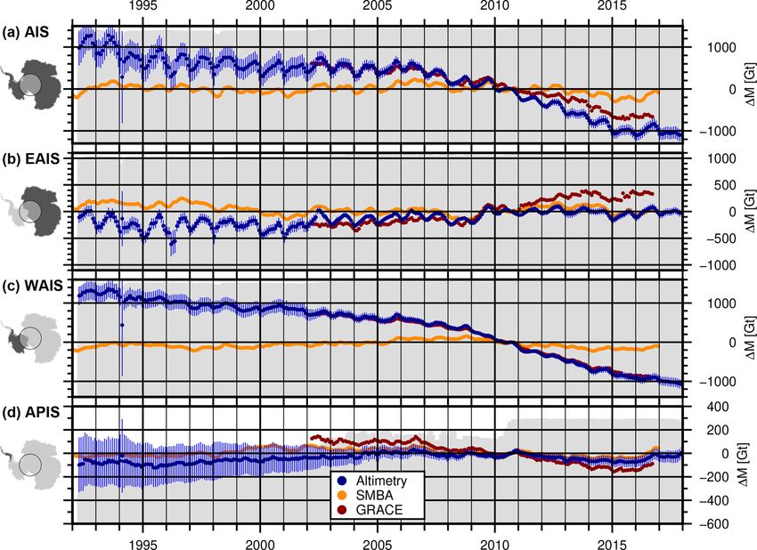
430                                                                  L. Schröder et al.: Multi-mission altimetry in Antarctica

offsets can be explained by the fact that for surfaces that un-
dulate within the ∼ 20 km beam-limited footprint, the radar
measurements tend to refer to local topographic maxima (the
POCA), while the validation data from ground-based GNSS
profiles or ICESat-based profiles represent the full topogra-
phy. The standard deviation of differences between RA data
and validation data contains information about the measure-
ment noise but is additionally influenced by the significantly
different sampling of a rough surface as well. While over flat
terrain, this standard deviation is below 50 cm for most satel-
                                                                     Figure 2. Precision of different processing versions of Envisat mea-
lite altimeter data sets, it can reach 10 m and more in coastal
                                                                     surements from near-time (< 31 days) crossovers, binned against
regions. However, both types of error relate to the different        slope. Red curve: ESA version with ICE-2 retracker and relocated
sampling of topography of the respective observation tech-           by mean surface slope. Light, medium and dark blue curves: data
niques. An elevation change, detected from within the same           reprocessed in this study with 50 %-, 20 %- and 10 %-threshold re-
technique, is not influenced by these effects. Hence, with re-       tracker, relocated using the refined method. Vertical bars: number
spect to elevation changes, not the accuracy but the precision       of crossovers for the ESA (red) and our 10 % threshold retracked
(i.e., the repeatability) has to be considered.                      data (blue).
   This precision can be studied using intra-mission
crossovers between ascending and descending profiles. Here,          Table 1. Noise level and slope-related component (s in degrees) of
the precision
         √      of a single measurement is obtained by σH =          the measurement precision, fitted to near-time crossovers (unit: m)
|1H |/ 2 as two profiles contribute to this difference. To           of the data from the respective data center and our reprocessed data
reduce the influence of significant real surface elevation           (with a 10 % threshold retracker applied).
changes between the two passes, we only consider crossovers
with a time difference of less than 31 days. In stronger in-               Data set                      Data center          Reprocessed
clined topography, the precision of the slope correction dom-
                                                                           Seasat                       0.21 + 1.91s 2        0.25 + 0.70s 2
inates the measurement error (Bamber, 1994). Hence, to pro-
                                                                           Geosat                       0.17 + 0.86s 2        0.18 + 1.16s 2
vide meaningful results, the surface slope needs to be taken
                                                                           ERS-1 (ocean)                0.25 + 0.90s 2        0.09 + 0.18s 2
into consideration. We calculate the slope from the CryoSat-
                                                                           ERS-1 (ice)                  0.36 + 2.37s 2        0.17 + 0.57s 2
2 DEM (Helm et al., 2014). The absence of slope-related ef-                ERS-2 (ocean)                0.23 + 0.75s 2        0.07 + 0.14s 2
fects on flat terrain allows for the study of the influence of the         ERS-2 (ice)                  0.38 + 2.57s 2        0.15 + 0.53s 2
retracker (denoted as noise here). With increasing slope, the              Envisat                      0.17 + 1.03s 2        0.05 + 0.37s 2
additional error due to topographic effects can be identified.             ICESat                       0.05 + 0.25s 2
   A comparison of the crossover errors of our reprocessed                 CryoSat-2 (LRM)              0.18 + 2.46s 2        0.03 + 1.06s 2
data and of the standard products shows significant improve-               CryoSat-2 (SARIn)            0.38 + 2.01s 2        0.11 + 0.79s 2
ments achieved by our reprocessing. Figure 2 shows this
                                                                         Note that the slope-dependent component is weakly determined for data
comparison for Envisat (similar plots for each data set can be           sets with poor tracking in rugged terrain such as Seasat, Geosat or the
found in Fig. S1), binned into groups of 0.05◦ of specific sur-          ERS ocean mode and for the LRM mode of CryoSat-2.
face slope. The results for a flat topography show that a 10 %
threshold provides the highest precision, which confirms the
findings of Davis (1997). For higher slopes, we see that our         provements. For the two early missions Seasat and Geosat,
refined slope correction also contributed to a major improve-        the crossover error of our reprocessed profiles is similar to
ment. A constant noise level σnoise and a quadratic, slope-          that of the original data set from GSFC. However, the num-
related term σslope have been fitted to the data according to        ber of crossover points is significantly increased, especially
σH = σnoise +σslope ·s 2 , where s is in the unit of degrees. The    for Geosat (see Fig. S1). This means that our reprocessing
results in Table 1 show that for each of the PLRA data sets          obtained reliable data where the GSFC processor rejected the
of ERS-1, ERS-2 and Envisat, the measurement noise could             measurements.
be reduced by more than 50 % compared to the ESA prod-                  In addition to measurement noise, reflected in the
uct which uses the functional fit retracker ICE-2 (Legrésy           crossover differences, a consistent pattern of offsets between
and Rémy, 1997). With respect to the CryoSat-2 standard re-          ascending and descending tracks has been observed previ-
tracker (Wingham et al., 2006a), the improvement is even             ously (A–D bias; Legrésy et al., 1999; Arthern et al., 2001).
larger. Improvements are also significant for the slope-related      Legrésy et al. (1999) interpret this pattern as an effect of the
component. For the example of Envisat and a slope of 1◦ , the        interaction of the linearly polarized radar signal with wind-
slope-related component is 1.03 m for the ESA product and            induced surface structures, while Arthern et al. (2001) at-
only 0.37 m for the reprocessed data. The advanced interfer-         tribute the differences to anisotropy within the snowpack.
ometric processing of the SARIn data achieved similar im-            Helm et al. (2014) showed that a low threshold retracker sig-

The Cryosphere, 13, 427–449, 2019                                                               www.the-cryosphere.net/13/427/2019/
L. Schröder et al.: Multi-mission altimetry in Antarctica                                                                      431

nificantly reduces the A–D bias. We observe a similar major         and Simonsen and Sørensen (2017) use two additional wave-
reduction (from ±1 m in some regions for a functional fit re-       form shape parameters, obtained from functional fit retrack-
tracker to ±15 cm when using a 10 % threshold; see Fig. S2).        ers. Nilsson et al. (2016) showed that a low threshold re-
The remaining bias is not larger, in its order of magnitude,        tracker mitigates the need for a complex waveform shape
than the respective noise. Moreover, near the ice sheet mar-        correction. Hence, we decided to use a solely backscatter-
gins, the determination of meaningful A–D biases is compli-         related correction.
cated by the broad statistical distribution of A–D differences         Besides the parameters in Eq. (1), McMillan et al. (2014)
and the difficulty of discriminating outliers. We therefore do      and Simonsen and Sørensen (2017) estimate an additional
not apply a systematic A–D bias as a correction but rather in-      orbit-direction-related parameter to account for A–D biases.
clude its effect in the uncertainty estimate of our final result.   In Sect. 2.3 we showed that these biases are significantly re-
                                                                    duced due to reprocessing with a low threshold retracker.
                                                                    A further reduction of possible remaining artifacts of A–
3     Multi-mission SEC time series                                 D biases is achieved by smoothing in the merging step in
                                                                    Sect. 3.3.3. The weighted averaging of the results over a di-
3.1    Repeat-track parameter fit
                                                                    ameter of 60 km leads to a balanced ratio of ascending and
We obtain elevation time series following the repeat-track          descending tracks. Our choices concerning the correction for
approach, similar to Legrésy et al. (2006) and Flament and          local topography, time-variable penetration effects and A–D
Rémy (2012). As the orbits of the missions used here have           biases were guided by the principle of preferring the simplest
different repeat-track patterns, instead of along-track boxes       viable model in order to keep the number of parameters small
we perform our fit on a regular grid with 1 km spacing (as in       compared to the number of observations.
Helm et al., 2014). For each grid cell we analyze all eleva-           In contrast to this single mission approach, here we per-
tion measurements hi within a radius of 1 km around the grid        form a combined processing of all data from different mis-
cell center. This size seems reasonable as for a usual along-       sions and even different altimeter techniques. Thus, some of
track spacing of about 350 m for PLRA (Rémy and Parouty,            the parameters may vary between the data sets. To allow for
2009), each track will have up to five measurements within          offsets between the missions, the elevation at the cell cen-
the radius. Due to the size of the pulse-limited footprint, a       ter a0 is fitted for each mission individually. The same ap-
smaller search radius would contain only PLRA measure-              plies to dBS, which might relate to specific characteristics of
ments with very redundant topographic information and thus          a mission as well. For Seasat, covering less than 100 days,
would not be suitable to fit a reliable correction for the to-      this parameter is not estimated, as we assume that during the
pography. As specified in Eq. (1), the parameters contain a         mission lifetime no significant changes occurred. For ICE-
linear trend (dh/dt), a planar topography (a0 , a1 , a2 ) and a     Sat, dBS is not estimated either, as signal penetration is neg-
regression coefficient (dBS) for the anomaly of backscattered       ligible for the laser measurements.
power (bsi − bs) to account for variations in the penetration          Between different observation techniques (i.e., PLRA,
depth of the radar signal.                                          SARIn and laser altimetry), the effective surface slope may
   For a single mission, the parameters are adjusted accord-        also differ. Considering the specific footprint sizes and
ing to the following model:                                         shapes, the topography is sampled in a completely different
                                                                    way as illustrated in Fig. 3. While PLRA refers to the clos-
hi =dh/dt (ti − t0 )+                                               est location anywhere within the ∼ 20 km beam-limited foot-
                                                                    print (i.e., the POCA), CryoSat’s SARIn measurement can be
      a0 + a1 xi + a2 yi +
                                                                   attributed within the narrow Doppler stripe in the cross-track
      dBS bsi − bs +                                                direction. For ICESat the ∼ 70 m laser spot allows a much
      resi .                                                 (1)    better sampling of local depressions. Hence, the slope pa-
                                                                    rameters a1 and a2 are estimated for each of the techniques
Here, ti denotes the time of the observation. The reference         independently.
epoch t0 is set to 09/2010. xi and yi are the polar stere-             Considering these sensor-specific differences, the model
ographic coordinates of the measurement location, reduced           for the least squares adjustment in Eq. (1) is extended for
by the coordinates of the cell’s center. The residual resi de-      multi-mission processing to
scribes the misfit between the observation and the estimated
                                                                    hi =dh/dt (ti − t0 )+
parameters.
   To account for varying penetration depths due to variations          a0,M(i) + a1,T (i) xi + a2,T (i) yi +
in the electromagnetic properties of the ice sheet surface,

                                                                        dBSM(i) bsi − bsM(i) +
different approaches exist. Wingham et al. (1998), Davis
                                                                        resi ,                                                 (2)
and Ferguson (2004), McMillan et al. (2014) and Zwally
et al. (2015) apply a linear regression using the backscat-         where M(i) and T (i) denote to which mission or technique
tered power. Flament and Rémy (2012), Michel et al. (2014)          the measurement hi belongs.

www.the-cryosphere.net/13/427/2019/                                                          The Cryosphere, 13, 427–449, 2019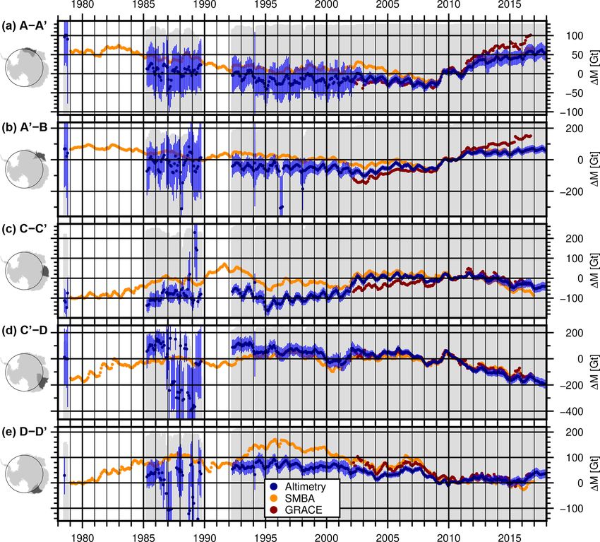
432                                                                        L. Schröder et al.: Multi-mission altimetry in Antarctica

                                                                           This recombination of parameters from Eq. (2) and averages
                                                                           of residuals does not include the parameters of topography
                                                                           slope and backscatter regression. Hence, each time series
                                                                           of hj,M relates to the cell center and is corrected for time-
                                                                           variable penetration effects. Due to the reference elevation
                                                                           a0,M , which may also contain the inter-mission offset, the
                                                                           penetration depth and a component of the topography sam-
                                                                           pling within the cell, this results in individual time series for
                                                                           each single mission. A schematic illustration of the results of
                                                                           this step is given in Fig. 5a. The temporal resolution of these
                                                                           time series is defined by using monthly averages of the resid-
                                                                           uals. With typical repeat-cycle periods of 35 days or more,
                                                                           these res typically represent the anomalies of a single satel-
                                                                           lite pass towards all parameters including the linear rate of
                                                                           elevation change. The standard deviation of the residuals in
Figure 3. Illustration of the technique-dependent topographic sam-         these monthly averages is used as uncertainty measure for
pling. The laser (red) measures the surface elevation in the nadir of      hj,M (see Sect. S3.1 for further details).
the instrument, while for radar altimetry (blue) the first return signal
originates from the POCA (marked by the blue point). Hence, pla-           3.3     Combination of the single-mission time series
nar surface approximations to the measured heights (dashed lines)
as in Eq. (2) are intrinsically different for the different techniques.    In order to merge data from different missions into a joint
                                                                           time series, inter-mission offsets have to be determined and
                                                                           eliminated. In the ERS reprocessing project (Brockley et al.,
   We define a priori weights for the measurements hi based                2017), mean offsets between the ERS missions and Envisat
on the precision of the respective mission and mode from                   have been determined and applied to the elevation data. How-
crossover analysis (Table 1) and depending on the surface                  ever, for ice sheet studies inter-satellite offsets are found to be
slope at the measurement location. This means that in re-                  regionally varying (Zwally et al., 2005; Thomas et al., 2008;
gions with a more distinctive topography, ICESat measure-                  Khvorostovsky, 2012). When merging data from different
ments (with a comparatively low slope-dependent error com-                 observation techniques (PLRA, SARIn and laser) the cali-
ponent) will obtain stronger weights, compared to PLRA as                  bration gets even more challenging. We chose an approach
Envisat. Over regions of flat topography, such as the interior             in different steps which is depicted in Figs. 4 and 5. The fol-
of East Antarctica, the weights between PLRA and ICESat                    lowing section gives an overview and explains the different
are comparable.                                                            steps to merge the single mission time series. A detailed de-
   In order to remove outliers from the data and the results we            scription of the parameters used in each step can be found in
apply different outlier filters. After the multi-mission fit, we           the Supplement.
screen the standardized residuals (Baarda, 1968) to exclude
any resi that exceed 5 times its a posteriori uncertainty. We              3.3.1    Merging PLRA time series
iteratively repeat the parameter fit until no more outliers are
found. Furthermore, in order to exclude remaining unrealis-                In the first step, we merge the PLRA time series. For these
tic results from further processing, we filter our repeat-track            missions the topographic sampling by the instruments is sim-
cells and reject any results where we obtain an absolute el-               ilar and thus the offsets are valid over larger regions. For
evation change rate |dh/dt| which is larger than 20 m yr−1                 overlapping missions (ERS-1, ERS-2, Envisat, CryoSat-2
or where the standard deviation of this rate is higher than                LRM) the offsets are calculated from simultaneous epochs
0.5 m yr−1 .                                                               (blue area in Fig. 5b), as performed by Wingham et al. (1998)
                                                                           or Paolo et al. (2016). Smoothed grids of these offsets are
                                                                           generated, summed up if necessary to make all data sets com-
3.2   Single-mission time series
                                                                           parable with Envisat (see Fig. S4) and applied to the respec-
                                                                           tive missions. For the ERS missions, we find significant dif-
After fitting all parameters according to the multi-mission
                                                                           ferences in the offsets for ice and ocean mode; hence, we de-
model (Eq. 2), we regain elevation time series by recombin-
                                                                           termine separate offsets for each mode. Comparing our maps
ing the parameters a0 and dh/dt with monthly averages of
                                                                           with similar maps of offsets between ERS-2 (ice mode) and
the residuals (res). For each month j and each mission M,
                                                                           Envisat shown by Frappart et al. (2016) reveals that the spa-
the time series are constructed as
                                                                           tial pattern agrees very well, but we find significantly smaller
                                                                           amplitudes. We interpret this as a reduced influence of vol-
hj,M = a0,M + dh/dt (tj − t0 ) + resj,M .                           (3)    ume scattering due to our low retracking threshold. In ac-

The Cryosphere, 13, 427–449, 2019                                                                www.the-cryosphere.net/13/427/2019/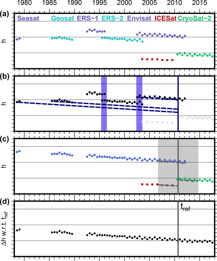
L. Schröder et al.: Multi-mission altimetry in Antarctica                                                                               433

Figure 4. Schematic diagram of the processing steps from the com-
bined repeat-track parameter fit over single-mission time series to-
wards a combined multi-mission time series.

cordance with Zwally et al. (2005), we did not find an ap-
propriate functional relationship between the offset and the
waveform parameters.
   To calibrate Geosat and Seasat, a gap of several years with-
out observations has to be bridged. As depicted by the dashed
blue lines in Fig. 5b, we do this using the trend-corrected ref-
erence elevations a0,M from the joint fit in Eq. (2). This, how-
ever, can only be done if the rate is sufficiently stable over the
whole period. Therefore, we use two criteria. First, we check          Figure 5. Schematic illustration of the combination of the missions.
the standard deviation of the fit of dh/dt. This σdh/dt indi-          (a) Single-mission time series of PLRA missions (blue and cyan),
cates the consistency of the observations towards a linear rate        CryoSat-2 in SARIn mode (green) and the laser altimetry measure-
during the observational period. However, anomalies dur-               ments of ICESat (red) with inter-mission offsets. (b) Offsets be-
ing the temporal gaps between the missions (i.e., 1978–1985            tween the PLRA data are determined from overlapping epochs (blue
and 1989–1992) cannot be detected in this way. Therefore,              area) or trend-corrected elevation differences (according to Eq. 2)
we further utilize a firn densification model (FDM; Ligten-            where dh/dt is sufficiently stable. (c) The specific offset between
berg et al., 2011; van Wessem et al., 2018). This model de-            PLRA, SARIn and laser data depends on the sampling of the topog-
                                                                       raphy within each single cell. These different techniques are aligned
scribes the anomalies in elevation due to atmospheric pro-
                                                                       by reducing each elevation time series by the specific elevation at
cesses against the long-term mean. The root mean square
                                                                       the reference epoch tref . Due to possible nonlinear surface elevation
(rms) of the FDM time series is hence a good measure for               changes, this reference elevation is obtained from an 8-year inter-
the magnitude of the nonlinear variations in surface eleva-            val only (gray area). (d) The combined multi-mission time series
tion. Consequently, only cells where σdh/dt < 1 cm yr−1 and            contains SECs with respect to tref .
rmsFDM < 20 cm, indicating a highly linear rate, are used to
calibrate the two historic missions. Maps of the offsets with
respect to Envisat are shown in Fig. S5. The FDM criterion
is not able to detect changes in ice dynamics. However, as             our final estimate of the offset, applied to the measurements,
regions where both stability criteria are fulfilled are mainly         is a constant, calculated as the average offset over the re-
found on the plateau where flow velocity is below 30 m yr−1            gions meeting the stability criterion. The spatial variability
(Rignot et al., 2017), we expect no significant nonlinear el-          not accounted for by the applied offset is included, instead,
evation changes due to ice flow. The mean of the offsets               in the assessed uncertainty. Our bias between Seasat and En-
over all cells amounts to −0.86 m for Seasat and −0.73 m               visat (−0.86 ± 0.85 m) agrees within uncertainties with the
for Geosat. The corresponding standard deviations of 0.85              ocean-based bias of −0.77 m used by Fricker and Padman
and 0.61 m are mainly a result of the regional pattern of              (2012). However, we prefer the offset determined over the ice
the offsets. The true offsets are likely to have spatial varia-        sheet because this kind of offset may depend on the reflecting
tions. However, we are not able to distinguish spatial vari-           medium (see Sect. S3.2.2 for a more detailed discussion).
ations of the offset from residual effects of temporal height             With the help of these offsets, all PLRA missions were
variations in the regions meeting the stability criterion. In          corrected towards the chosen reference mission Envisat. Un-
the regions not meeting this criterion, we are not able to es-         certainty estimates of the offsets are applied to the respective
timate the spatial variations of the offset at all. Therefore,         time series to account for the additional uncertainty. Hence,

www.the-cryosphere.net/13/427/2019/                                                              The Cryosphere, 13, 427–449, 2019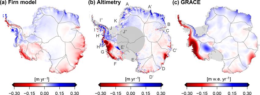
434                                                                L. Schröder et al.: Multi-mission altimetry in Antarctica

the PLRA time series are combined (blue in Fig. 5c with ad-        (which is about the size of a beam-limited radar footprint).
ditional CryoSat-2 LRM mode where available). At epochs            The five examples in Fig. 6 demonstrate the spatiotemporal
when more than one data set exists, we apply weighted aver-        coverage of the resulting SEC grids at different epochs. The
aging using the uncertainty estimates.                             corresponding uncertainty estimates, given in Fig. 6b (further
                                                                   details in the Supplement), reach values of 1 m and more.
3.3.2   Technique-specific surface elevation changes               Besides the measurement noise and the uncertainties of the
                                                                   offsets, these uncertainty estimates contain a further compo-
In contrast to the PLRA data in the previous step, when            nent from the weighted averaging. In regions with large vari-
merging data from different observation techniques such as         ations in 1h over relatively short spatial scales (such as at
CryoSat’s SARIn mode, ICESat’s laser observations and              fast-flowing outlet glaciers), such variations can add a sig-
PLRA, the different sampling of topography also has to be          nificant contribution to σ1h . As the magnitude of 1h grows
considered. As noted in Sect. 3.1, this might lead to com-         with the temporal distance to the reference epoch, the largest
pletely different surfaces fitted to each type of elevation mea-   contributions to σ1h can be expected for the earliest epochs.
surement and the time series need to be calibrated for each        This also explains why the epoch 09/2008 provides the low-
cell individually. However, not all cells have valid observa-      est uncertainty estimate in these examples, even lower than
tions of each data set. Therefore, instead of calibrating the      the CryoSat-2-based epoch 09/2017.
techniques against each other, we reduce each time series
by their elevation at a common reference epoch and hence
obtain time series of surface elevation changes (SEC) with         4     Comparison of SEC with independent data
respect to this reference epoch instead of absolute elevation
time series. This step eliminates offsets due to differences in    4.1    In situ and airborne observations
firn penetration or due to the system calibration between the
techniques as well.                                                To validate our results, we used inter-profile crossover differ-
   We chose September 2010 (09/2010) as the reference              ences of 19 kinematic GNSS profiles (available for download
epoch. This epoch is covered by the observational periods          from Schröder et al., 2016) and elevation differences from
of PLRA and CryoSat SARIn and also is exactly 1 year after         Operation IceBridge (OIB ATM L4; Studinger, 2014). The
the last observations of ICESat, which reduces the influence       ground-based GNSS profiles were observed between 2001
of an annual cycle. As discussed in Sect. 3.3.1, nonlinear ele-    and 2015 on traverse vehicles of the Russian Antarctic Ex-
vation changes will adulterate a0 from Eq. (2), obtained over      pedition and most of them covered more than 1000 km. The
the full time span. Therefore, we applied another linear fit       accuracy of these profiles has been determined in Schröder
to a limited time interval of 8 years only (September 2006–        et al. (2017) to 4–9 cm. One profile (K08C) has not been used
September 2014, gray area in Fig. 5c). We subtract the vari-       due to poorly determined antenna height offsets. For each
ation of the FDM over this period to account for short-term        crossover difference between kinematic profiles from differ-
variations. The limited time interval reduces the influence of     ent years, we compare the differences of the correspond-
changes in ice dynamics. We estimate the individual refer-         ing altimetric SEC epochs in this location (δ1h = 1hKIN −
ence elevations a0,T for each technique T and a joint dh/dt.       1hALT ). The same analysis has been performed with the el-
After subtracting the technique-specific reference elevations      evation changes obtained from differences of measurements
a0,T from the respective time series, they all refer to 09/2010    of the scanning laser altimeter (Airborne Topographic Map-
and can be combined.                                               per, ATM) of OIB. As described by Studinger (2014), the
                                                                   Level 4 1h product is obtained by comparing planes fitted
3.3.3   Merging different techniques                               to the laser scanner point clouds. The flights, carried out be-
                                                                   tween 2002 and 2016, were strongly concentrated along the
We perform the final combination of the techniques using           outlet glaciers of West Antarctica and the Antarctic Penin-
a weighted spatiotemporal averaging with 10 km σ Gaus-             sula. Hence, they cover much more rugged terrain, which
sian weights in the spatial domain (up to a radius of 3σ =         is more challenging for satellite altimetry. Over the tribu-
30 km) and over 3 epochs (i.e., including the two consecutive      taries of the Amundsen Sea glaciers and along the polar gap
epochs) in the temporal domain. Hence, we obtain grids of          of ICESat, some repeated measurements have also been per-
surface elevation change (SEC) with respect to 09/2010 for         formed over flat terrain. The accuracy of these airborne mea-
each month observed. Due to the smoothing of the weight-           surements has been validated, e.g., near summit station in
ing function, we reduce our spatial SEC grid resolution to         Greenland. Brunt et al. (2017) used ground-based GNSS pro-
10 km × 10 km. The respective uncertainties are calculated         files of snowmobiles for this task and obtained offsets on the
according to the error propagation. To avoid extrapolation         order of only a few centimeters and standard deviations be-
and to limit this merging step to the observed area only, we       tween 4 and 9 cm.
calculate a value for an epoch in the 10 km × 10 km grid cells        Figure 7a and d show the results of our validation (more
only if we have data within 20 km around the cell center           detailed maps for several regions at Fig. S6). A satellite cal-

The Cryosphere, 13, 427–449, 2019                                                       www.the-cryosphere.net/13/427/2019/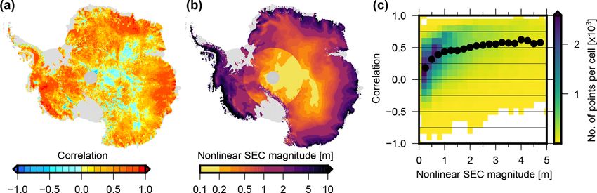
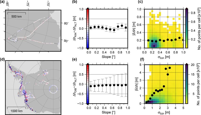
L. Schröder et al.: Multi-mission altimetry in Antarctica                                                                                435

Figure 6. Five example snapshots of the resulting combined surface elevation time series (a) and their corresponding uncertainty (b). The
height differences refer to our reference epoch 09/2010.

Figure 7. Validation with elevation differences observed by kinematic GNSS between 2001 and 2015 (a, b, c) and Operation IceBridge
between 2002 and 2016 (d, e, f). Differences between elevation changes observed by the validation data and altimetry are shown in the maps
(a, d, color scale in panels b and e). Median and MAD of these differences, binned by different surface slope, are shown in the center (b, e).
The right diagrams (c, f) show the comparison of these differences with the respective uncertainty estimate, obtained from both data sets.
The point density is plotted from yellow to blue and the black dots show the root mean square, binned against the estimated uncertainty.

ibration error would lead to systematic biases between the               variation with slope. The IceBridge data cover the margins of
observed elevation differences if 1hALT is obtained from                 many West Antarctic glaciers, where elevation changes differ
data of two different missions. However, such biases may                 over relatively short distances. Hence, it is not surprising that
also be caused by systematic errors in the validation data.              we see a significantly larger spread of δ1h at higher slopes
Furthermore, in contrast to the calibration data, the RA mea-            here. However, in the less inclined regions, the MAD of the
surements may systematically miss some of the most rapid                 differences is still at a level of 25 cm, which is significantly
changes if those are located in local depressions (Thomas                larger than in the comparison with the GNSS profiles. This
et al., 2008). With an overall median difference of 6 ± 10 cm            large spread for regions with low slopes originates mainly
for the GNSS profiles and −9 ± 42 cm for OIB, however, the               from the tributaries of Pine Island Glacier, where many cam-
observed elevation changes show only moderate systematic                 paigns of OIB are focused (see Figs. 7d and S6d for details).
effects and agree within their error bars. The median absolute           While still relatively flat, the surface elevation in this area
deviation (MAD) for different specific surface slopes (Fig. 7b           is comparatively low, which leads to a stronger influence of
and e) reveals the influence of topography in this validation.           precipitation (Fyke et al., 2017). This induces higher short-
The GNSS profiles show only a very small increase of this                term variations in surface elevation, which might explain the

www.the-cryosphere.net/13/427/2019/                                                                 The Cryosphere, 13, 427–449, 2019
436                                                                L. Schröder et al.: Multi-mission altimetry in Antarctica

higher differences between the IceBridge results and our 3-        for the period 1992–2016 (depicted in Fig. S7). The trends
month temporally smoothed altimetry data. In contrast, the         are only calculated from epochs where both data sets have
differences around the South Pole or in Queen Elizabeth            data; i.e., in the polar gap this comparison is limited to 2003–
Land (see also Fig. S6c) are significantly smaller. For the        2016 or 2010–2016, depending on the first altimetry mission
2016 campaign of OIB, Brunt et al. (2018) furthermore re-          providing data here. After the detrending, the anomalies are
port a spurious elevation variation of 10 to 15 cm across the      used to calculate correlation coefficients for each cell, de-
wide-scan ATM swath, which indicates a bias in the instru-         picted in Fig. 8a. Figure 8b shows the average magnitude of
mental tilt angle. This could explain the systematic differ-       the seasonal and interannual variations (nonlinear SEC), cal-
ences along the 88◦ S circle profiles where this campaign is       culated as the rms of the anomalies from the altimetry data.
involved.                                                          Comparing the two maps shows that the correlation is around
   The observed δ1h can further be used to evaluate the un-        0.5 or higher, except in regions where the magnitude of the
certainty estimates. In Fig. 7c and f, the uncertainty estimates   anomalies is small (i.e., where the signal-to-noise ratio of the
of the four contributing data sets are combined and compared       altimetric data is low) and where large accelerations in ice ve-
to the observed differences. The comparison with both vali-        locity are observed (such as near the grounding zone of Pine
dation data sets supports the conclusion that the uncertainty      Island Glacier). The relationship between the correlation co-
estimates are reasonable. For 1hALT we expect higher er-           efficient and the magnitude of the nonlinear SEC is depicted
rors in coastal regions due to the increased uncertainty of the    in Fig. 8c, where we see that for the vast majority of cells the
topographic correction in radar altimetry. A similar relation      correlation is positive. For anomalies with a nonlinear SEC
to topography is expected for 1hOIB due to the plane fit to        > 0.5 m, the average correlation is between 0.3 and 0.6.
the ATM point cloud, but surface roughness and crevassing             Anomalies against the simultaneously observed long-term
also play an important role here. In contrast, the errors of the   trend (1992–2016) can also be computed for earlier epochs.
GNSS-derived 1hKIN are almost independent of topography.           Assuming no significant changes in ice dynamics here, these
Instead, 1hKIN tends to be more uncertain on the plateau,          anomalies allow for a comparison of Geosat and Seasat with
where the soft snow causes large variations of the subsidence      the FDM. The median difference between the anomalies ac-
of the vehicles into the upper firn layers. The relatively low     cording to Geosat and the anomalies according to the FDM
differences in δ1h, even in regions that imply a higher un-        amounts to 0.12 ± 0.21 m (see Fig. S8). Considering that this
certainty, are likely just incidental for the small sample of      difference is very sensitive to extrapolating the long-term
validation data along the GNSS profiles.                           trends, this is a remarkable agreement. With a median of
   In conclusion, this validation shows that remaining sys-        0.26±0.32 m, the difference between anomalies from Seasat
tematic biases (originating from satellite altimetry or the val-   and from the FDM is larger, but this comparison is also more
idation data) are less than a decimeter in the observed re-        vulnerable to potential errors due to the extrapolation. As
gions and that our uncertainty estimate is realistic. However,     the FDM starts in 1979 while Seasat operated in 1978, we
only altimetric SEC within the interval 2001–2016 can be           compare the Seasat data with the FDM anomalies from the
validated in this way. For the earlier missions, no spatially      respective months of 1979, which might impose additional
extensive high-precision in situ data are publicly available.      differences. Finally, the FDM model has its own inherent er-
                                                                   rors and uncertainties. Therefore, only part of the differences
4.2   Firn model                                                   originate from errors in the altimetry results.

Another data set, which covers almost the identical spatial
and temporal range as the altimetric data, is the IMAU Firn        5     Results
Densification Model (FDM; Ligtenberg et al., 2011), forced
at the upper boundary by the accumulation and temperature          5.1    Surface elevation changes
of the Regional Atmospheric Climate Model, version 2.3p2
(van Wessem et al., 2018). The IMAU-FDM has been up-               The average rates of elevation change over different time in-
dated to the period 1979–2016, modeling the firn properties        tervals of our multi-mission time series are shown in Fig. 9.
and the related surface elevation changes on a 27 km grid.         To calculate these rates, we first averaged the data over the
However, as the FDM contains elevation anomalies only,             first year and the last year of the interval to reduce the noise,
any long-term elevation trend over 1979–2016, e.g., due to         then subtracted the respective averages from each other and
changes in precipitation on longer timescales (for example         finally divided these differences by their time difference in
those observed in some regions of West Antarctica; Thomas          years. If one of the years does not cover the full annual cy-
et al., 2015) would not be included in the model. Further-         cle, we calculate the average only from the months covered
more, due to the nature of the model, it cannot give infor-        in both years (July–October for 1978–2017, April–December
mation about ice dynamic thinning and thickening. Hence,           for 1992–2017). We calculate the SEC rate from epoch dif-
to compare the FDM and the SEC from altimetry, we first            ferences instead of fitting a rate to all epochs because the
remove a linear trend from both data sets. This is performed       first observations at specific latitudes start in different years,

The Cryosphere, 13, 427–449, 2019                                                        www.the-cryosphere.net/13/427/2019/
L. Schröder et al.: Multi-mission altimetry in Antarctica 437 Figure 8. (a) Correlation coefficient between the SEC anomalies of the altimetry grids and the FDM over 1992–2016 after detrending. (b) Av- erage magnitude of anomalies of the altimetry time series. (c) Correlation coefficient plotted against the nonlinear SEC. The point density is color coded from yellow to blue. The black dots show the binned mean values. Figure 9. Multi-mission surface elevation change from the combined SEC time series over different time intervals. (a, b) The long-term surface elevation change between 1978 and 2017 and 1992 and 2017 for the covered area. (c–j) Elevation change over consecutive time intervals reveals the interannual variability. Thin lines mark the drainage basin outlines, denoted in panel (a). Bold letters in boxes in panel (b) denote areas mentioned in the text and in Fig. 10. the observations have different precisions and the large gap 60 % of East Antarctica north of 81.5◦ S shows surface eleva- between 1978 and 1985 is not covered by observations at tion changes of less than ±1 cm yr−1 . Several coastal regions all. These three points would lead to a bias towards the later of the EAIS, however, show significant elevation changes. epochs in a fit, so that the rates would not be representative Totten Glacier (T in Fig. 9b) is thinning at an average rate for the true average elevation change over the full interval. of 72 ± 18 cm yr−1 at the grounding line (cf. Fig. 10b). Sev- The long-term elevation changes over 25 years (Fig. 9b) eral smaller glaciers in Wilkes Land also show a persistent show the well known thinning in the Amundsen Sea Em- thinning. We observe SEC rates of −26±10 cm yr−1 at Den- bayment and at Totten Glacier, as well as the thicken- man Glacier (D), −41 ± 19 cm yr−1 at Frost Glacier (F) and ing of Kamb Ice Stream (see, e.g., Wingham et al., 2006b; −33 ± 12 cm yr−1 near Cook Ice Shelf (C). Rignot (2006) Flament and Rémy, 2012; Helm et al., 2014). In contrast, showed that the flow velocity of these glaciers, which are www.the-cryosphere.net/13/427/2019/ The Cryosphere, 13, 427–449, 2019
438                                                                     L. Schröder et al.: Multi-mission altimetry in Antarctica

                                                                        1992–2017 interval, which indicates a persistent rate of thin-
                                                                        ning. Another benefit of our merged time series is that they
                                                                        allow for the calculation of rates over any subinterval, in-
                                                                        dependent of mission periods as demonstrated in Fig. 9c–j.
                                                                        For most of the coastal regions of the AIS, these rates over
                                                                        different intervals reveal that there is significant interannual
                                                                        variation. Such large-scale fluctuations in elevation change
                                                                        have been previously reported by Horwath et al. (2012) and
                                                                        Mémin et al. (2015) for the Envisat period. Our combined
                                                                        multi-mission time series now allow a detailed analysis of
                                                                        such signals on a temporal scale of up to 40 years.
                                                                           Four examples for elevation change time series in the re-
                                                                        sulting multi-mission SEC grids are shown in Fig. 10 (coor-
                                                                        dinates in Table S2). Pine Island Glacier (PIG) is located in
                                                                        the Amundsen Sea Embayment, which is responsible for the
                                                                        largest mass losses of the Antarctic Ice Sheet (e.g., McMil-
                                                                        lan et al., 2014). In East Antarctica, the largest thinning rates
                                                                        are observed at Totten Glacier. The region of Dronning Maud
                                                                        Land and Enderby Land in East Antarctica has been chosen
                                                                        as an example for interannual variation. Here, Boening et al.
                                                                        (2012) reported two extreme accumulation events in 2009
                                                                        and 2011, which led to significant mass anomalies. We chose
                                                                        a profile at Shirase Glacier as an example for this region. In
                                                                        contrast to the previous locations, a very stable surface ele-
                                                                        vation has been reported for Lake Vostok (e.g., Richter et al.,
                                                                        2014). This stability, however, has been a controversial case
                                                                        recently (Zwally et al., 2015; Scambos and Shuman, 2016;
                                                                        Richter et al., 2016). Therefore, our results in this region shall
                                                                        add further evidence that pinpoints the changes there.
                                                                           For Pine Island Glacier (Fig. 10a), we observe a continu-
                                                                        ous thinning over the whole observational period since 1992
Figure 10. Multi-mission SEC time series in four selected regions       (Seasat and Geosat measurements did not cover this region).
(a) Pine Island Glacier, (b) Totten Glacier, (c) Shirase Glacier in     Close to the grounding line (point D) the surface elevation
Dronning Maud Land and (d) Lake Vostok (marked by P, T, S and           has decreased by −45.8 ± 7.8 m since 1992, which means
V in Fig. 9b). The time series of points B, C and D are shifted along   an average SEC rate of −1.80 ± 0.31 m yr−1 . The time se-
1h for better visibility and the one σ uncertainty range is displayed
                                                                        ries reveals that this thinning was not constant over time,
in black. The maps on the left show the elevation change rate be-
                                                                        but accelerated significantly around 2006. The mean rate
tween 1992 and 2017 as in Fig. 9b (but in a different color scale).
                                                                        at D over 1992–2006 of −1.32 ± 0.66 m yr−1 increased to
                                                                        −4.17 ± 1.67 m yr−1 over 2007–2010. After 2010, the thin-
                                                                        ning rates near the grounding line decelerate again and for
grounded well below sea level, was above the balance veloc-             the period 2013–2017, the rate at D of −1.31 ± 0.80 m yr−1
ity for many years. Miles et al. (2018) analyzed satellite im-          is very close to the rate preceding the acceleration. Also,
ages since 1973 and found that the flow velocity of Cook Ice            at greater distances from the grounding line (B at 80 km,
Shelf glaciers has significantly accelerated since then. In con-        A at 130 km) we observe an acceleration of the prevailing
trast, the western sector of the EAIS (Coats Land, Dronning             rates around 2006 (−0.44 ± 0.15 m yr−1 over 1992–2006,
Maud Land and Enderby Land; basins J”–B) shows thicken-                 −1.20±0.10 m yr−1 over 2006–2017 at A). In contrast to the
ing over the last 25 years at rates of up to a decimeter per            points near the grounding line, further inland the thinning has
year.                                                                   not decelerated so far and is still at a high level. Hence, for
   Comparing the long-term elevation changes over 40 years              the most recent period (2013–2017) the elevation at all points
(Fig. 9a) with those over 25 years shows the limitations of the         along the 130 km of the main flow line is decreasing at very
early observations, but also the additional information they            similar rates. A similar acceleration of the elevation change
provide. There were relatively few successful observations              rate near the grounding line, followed by slowdown, is ob-
at the margins. However, for Totten and Denman glaciers,                served by Konrad et al. (2016). The onset of this acceleration
the 40-year rates at a distance of approximately 100 km in-             coincides with the detaching of the ice shelf from a pinning
land from the grounding line are similar to the rates over the          point (Rignot et al., 2014). For the time after 2009, Joughin

The Cryosphere, 13, 427–449, 2019                                                             www.the-cryosphere.net/13/427/2019/
You can also read