COVID-19 Public Sentiment Insights and Machine Learning for Tweets Classification - MDPI
←
→
Page content transcription
If your browser does not render page correctly, please read the page content below
information
Article
COVID-19 Public Sentiment Insights and Machine
Learning for Tweets Classification
Jim Samuel 1, * , G. G. Md. Nawaz Ali 2, * , Md. Mokhlesur Rahman 3,4 , Ek Esawi 5
and Yana Samuel 6
 1   Department of Business Analytics, University of Charleston, Charleston, WV 25304, USA
 2   Department of Applied Computer Science, University of Charleston, Charleston, WV 25304, USA
 3   The William States Lee College of Engineering, University of North Carolina at Charlotte,
     Charlotte, NC 28223, USA; mrahma12@uncc.edu
 4   Department of Urban and Regional Planning (URP), Khulna University of Engineering & Technology
     (KUET), Khulna 9203, Bangladesh
 5   Department of Data Analytics, University of Charleston, Charleston, WV 25304, USA; eesawi@ucwv.edu
 6   Department of Education, Northeastern University, Boston, MA 02115, USA; yana.samuel@gmail.com
 *   Correspondence: jim@aiknowledgecenter.com (J.S.); ggmdnawazali@ucwv.edu (G.G.M.N.A.)

 Received: 28 April 2020; Accepted: 9 June 2020; Published: 11 June 2020

 Abstract: Along with the Coronavirus pandemic, another crisis has manifested itself in the form
 of mass fear and panic phenomena, fueled by incomplete and often inaccurate information.
 There is therefore a tremendous need to address and better understand COVID-19’s informational
 crisis and gauge public sentiment, so that appropriate messaging and policy decisions can be
 implemented. In this research article, we identify public sentiment associated with the pandemic
 using Coronavirus specific Tweets and R statistical software, along with its sentiment analysis
 packages. We demonstrate insights into the progress of fear-sentiment over time as COVID-19
 approached peak levels in the United States, using descriptive textual analytics supported by
 necessary textual data visualizations. Furthermore, we provide a methodological overview of
 two essential machine learning (ML) classification methods, in the context of textual analytics,
 and compare their effectiveness in classifying Coronavirus Tweets of varying lengths. We observe a
 strong classification accuracy of 91% for short Tweets, with the Naïve Bayes method. We also observe
 that the logistic regression classification method provides a reasonable accuracy of 74% with shorter
 Tweets, and both methods showed relatively weaker performance for longer Tweets. This research
 provides insights into Coronavirus fear sentiment progression, and outlines associated methods,
 implications, limitations and opportunities.

 Keywords: COVID-19; Coronavirus; machine learning; sentiment analysis; textual analytics; twitter

1. Introduction
     In this research article, we cover four critical issues: (1) public sentiment associated with the
progress of Coronavirus and COVID-19, (2) the use of Twitter data, namely Tweets, for sentiment
analysis, (3) descriptive textual analytics and textual data visualization, and (4) comparison of
textual classification mechanisms used in artificial intelligence (AI). The rapid spread of Coronavirus
and COVID-19 infections have created a strong need for discovering efficient analytics methods
for understanding the flow of information and the development of mass sentiment in pandemic
scenarios. While there are numerous initiatives analyzing healthcare, preventative, care and recovery,
economic and network data, there has been relatively little emphasis on the analysis of aggregate
personal level and social media communications. McKinsey [1] recently identified critical aspects

Information 2020, 11, 314; doi:10.3390/info11060314                        www.mdpi.com/journal/information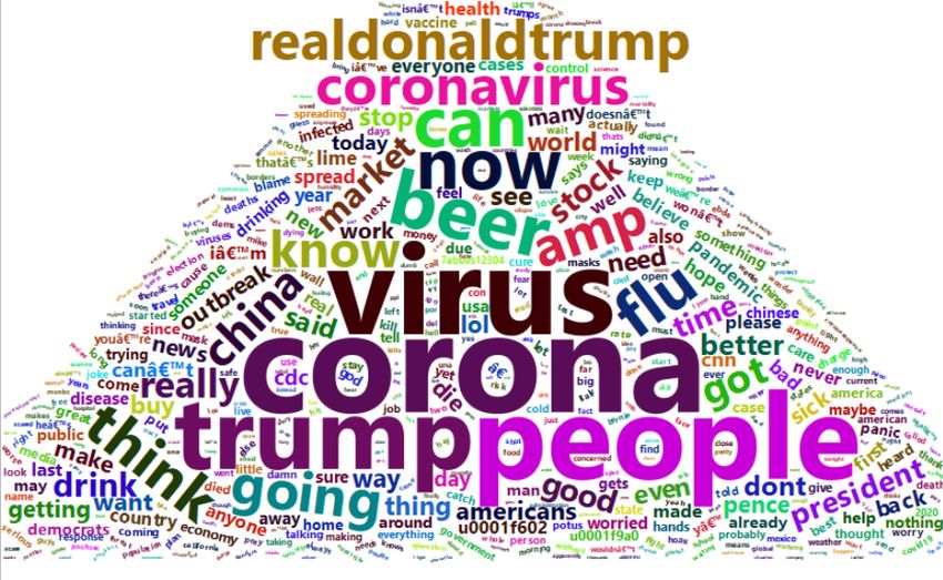
Information 2020, 11, 314                                                                                                  2 of 22

for COVID-19 management and economic recovery scenarios. In their industry-oriented report,
they emphasized data management, tracking and informational dashboards as critical components of
managing a wide range of COVID-19 scenarios.
     There has been an exponential growth in the use of textual analytics, natural language processing
(NLP) and other artificial intelligence techniques in research and in the development of applications.
Despite rapid advances in NLP, issues surrounding the limitations of these methods in deciphering
intrinsic meaning in text remain. Researchers at CSAIL, MIT (Computer Science and Artificial
Intelligence Laboratory, Massachusetts Institute of Technology), demonstrated how even the most
recent NLP mechanisms can fall short and thus remain “vulnerable to adversarial text” [2]. It is,
therefore, important to understand inherent limitations of text classification techniques and relevant
machine learning algorithms. Furthermore, it is important to explore whether multiple exploratory,
descriptive and classification techniques contain complimentary synergies which will allow us to
leverage the “whole is greater than the sum of its parts” principle in our pursuit for artificial intelligence
driven insights generation from human communications. Studies in electronic markets demonstrated
the effectiveness of machine learning in modeling human behavior under complex informational
conditions, highlighting the role of the nature of information in affecting human behavior [3].
The source data for all Tweets data analysis, tables and every figure, including the fear curve in
Figure 1 below, in this research consists of publicly available Tweets data, specifically downloaded for
the purposes of this research and further described in the Data acquisition and preparation Section 3.1.1
of this study.

                                                                COVID−19's Sentiment Curve: The Fear Pandemic
                                               600
                                               500
                 Fear Sentiment Tweets Count

                                               400
                                               300
                                               200
                                               100
                                               0

                                                     20−02−20      Fear Sentiment in Public Tweets              29−02−20

                                                                  Figure 1. Fear curve.

     The rise in emphasis on AI methods for textual analytics and NLP followed the tremendous
increase in public reliance on social media (e.g., Twitter, Facebook, Instagram, blogging, and LinkedIn)
for information, rather than on the traditional news agencies [4–6]. People express their opinions,
moods, and activities on social media about diverse social phenomena (e.g., health, natural hazards,
cultural dynamics, and social trends) due to personal connectivity, network effects, limited costs
and easy access. Many companies are using social media to promote their product and service
to the end-users [7]. Correspondingly, users share their experiences and reviews, creating a rich
reservoir of information stored as text. Consequently, social media and open communication platforms
are becoming important sources of information for conducting research, in the contexts of rapid
development of information and communication technology [8]. Researchers and practitioners mine
massive textual and unstructured datasets to generate insights about mass behavior, thoughts and
emotions on a wide variety of issues such as product reviews, political opinions and trends,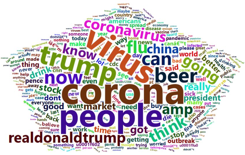
Information 2020, 11, 314 3 of 22
motivational principles and stock market sentiment [4,9–13]. Textual data visualization is also used to
identify the critical trend of change in fear-sentiment, using the “Fear Curve” in Figure 1, with the
dotted Lowess line demonstrating the trend, and the bars indicating the day to day increase in fear
Tweets count. Tweets were first classified using sentiment analysis, and then the progression of
the fear-sentiment was studied, as it was the most dominant emotion across the entire Tweets data.
This exploratory analysis revealed the significant daily increase in fear-sentiment towards the end of
March 2020, as shown in Figure 1.
In this research article, we present textual analyses of Twitter data to identify public sentiment,
specifically, tracking the progress of fear, which has been associated with the rapid spread of
Coronavirus and COVID-19 infections. This research outlines a methodological approach to analyzing
Twitter data specifically for identification of sentiment, key words associations and trends for crisis
scenarios akin to the current COVID-19 phenomena. We initiate the discussion and search for insights
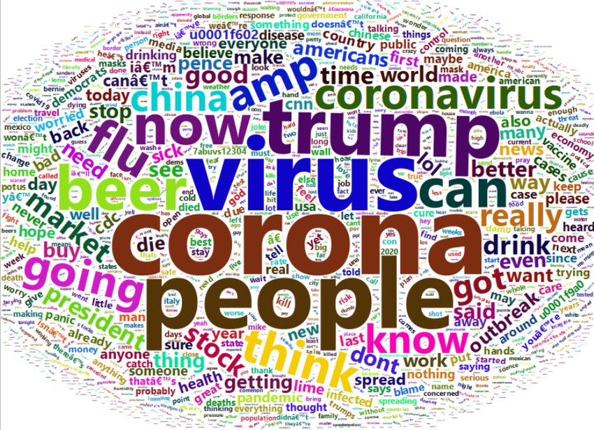
with descriptive textual analytics and data visualization, such as exploratory Word Clouds and
sentiment maps in Figures 2–4.
democrats
chinese beer
vaccine stock
since economy
worry
even
time
need little
virus
hope money
president
disease amp last public
bad next infected
person
everyone big
realdonaldtrump
getting probably
says things health already
charge this flu made
please come got
state
today
many
can due may
enough anyone
drinking
long
mask
don
cure must control case
stop
making
actually
america
thought
make con stay better
help buy told americans masks
want panic
died
cnn
catch
way
lol
great best someone kill government name coming
new hands
f602 travel tell
isn potus maybe response drink thing
yet wall good days
love now didn wouldn
really
mike said
man
gets
die think let
7abuvs12304
feel pence
spread usa joke won well media you deaths
heard
week
real
going f9a0 worse how started doesn know
else
country
pandemic
viruses care
year trump keep serious look news
away election give
cause job mexico
anything believe que
rate put worried also sure
home work there
talking first coronavirus another
cases world might
the
god sick
spreading never nothing back blame use
damn
outbreak lime
american saying china
something market cdc
what everything day
trying around open ever
cold people find
corona
Figure 2. An instance of word cloud in twitter data.
Early stage exploratory analytics of Tweets revealed interesting aspects, such as the relatively
higher number of Coronavirus Tweets coming from iPhone users, as compared to Android users,
along with a proportionally higher use of word-associations with politics (mention of Republican
and Democratic party leaders), URLs and humour, depicted by the word-association of beer with
Coronavirus, as summarized in Table 1 below. We observed that such references to humour and beer
were overtaken by “Fear Sentiment” as COVID-19 progressed and its seriousness became evident
(Figure 1). Tweets insights with textual analytics and NLP thus serve as a good reflector of shifts in
public sentiment.
Table 1. Tweet features summarized by source category.
Source Total Hashtags Mentions Urls Pols Corona Flu Beer AbuseW
iPhone 3281 495 2305 77 218 4238 171 336 111
Android 1180 149 1397 37 125 1050 67 140 41
iPad 75 6 96 4 12 85 4 8 2
Cities 30 0 0 0 0 0 0 0 0
One of the key contributions of this research is our discussion, demonstration and comparison
of Naïve Bayes and Logistic methods-based textual classification mechanisms commonly used in AIInformation 2020, 11, 314 4 of 22
applications for NLP, and specifically contextualized in this research using machine learning for Tweets
classifications. Accuracy is measured by the ratio of correct classifications to the total number of test
items. We observed that Naïve Bayes is better for small to medium size tweets and can be used for
classifying short Coronavirus Tweets sentiments with an accuracy of 91%, as compared to logistic
regression with an accuracy of 74%. For longer Tweets, Naïve Bayes provided an accuracy of 57% and
logistic regression provided an accuracy of 52%, as summarized in Tables 6 and 7.
2. Literature Review
This study was informed by research articles from multiple disciplines and therefore, in this
section, we cover literature review of textual analytics, sentiment analysis, Twitter and NLP,
and machine learning methods. Machine learning and strategic structuring of information
characteristics are necessary to address evolving behavioral issues in big data [3]. Textual analytics
deals with the analysis and evocation of characters, syntactic features, semantics, sentiment and
visual representations of text, its characteristics, and associated endogenous and exogenous features.
Endogenous features refer to aspects of the text itself, such as the length of characters in a social media
post, use of keywords, use of special characters and the presence or absence of URL links and hashtags,
as illustrated for this study in Table 2. These tables summarize the appearances of “mentions” and
“hashtags” in descending order, indicating the use of screen names and “#” symbol within the text of
the Tweet, respectively.
Table 2. Summary of endogenous features.
Tagged Frequency Hashtag Frequency
realDonaldTrump 74 coronavirus 23
CNN 21 DemDebate 16
ImtiazMadmood 16 corona 8
corona 13 CoronavirusOutbreak 8
AOC 12 CoronaVirusUpdates 7
coronaextrausa 12 coronavirususa 7
POTUS 12 Corona 6
CNN MSNBC 11 COVID19 5
Exogenous variables, in contrast, are those aspects which are external but related to the text, such
as the source device used for making a post on social media, location of Twitter user and source types,
as illustrated for this study in Table 3. The Table summarizes “source device” and “screen names”,
indicating variables representing type of device used post the Tweet, and the screen name of the Twitter
user, respectively, both external to the text of the Tweet. Such exploratory summaries describe the
data succinctly, provide a better understanding of the data, and helps generate insights which inform
subsequent classification analysis. Past studies explored custom approaches to identifying constructs
such as dominance behavior in electronic chat, indicating the tremendous potential for extending such
analyses by using machine learning techniques to accelerate automated sentiment classification and
the subsections that follow present key insights gained from literature review to support and inform
the textual analytics processes used in this study [14–17].Information 2020, 11, 314 5 of 22
Table 3. Summary of exogenous features.
Source Frequency Screen Name Frequency
Twitter for iPhone 3281 _CoronaCA 30
Twitter for Android 1180 MBilalY 25
Twitter for iPad 75 joanna_corona 17
Cities 30 eads_john 13
Tweetbot for iS 29 _jvm2222 11
CareerArc2.0 14 AlAboutNothing 11
Twitter Web Client 16 dallasreese 9
511NY-Tweets 3 CpaCarter 8
2.1. Textual Analytics
A diverse array of methods and tools were used for textual analytics, subject to the nature
of the textual data, research objectives, size of dataset and context. Twitter data has been used
widely for textual and emotions analysis [18–20]. In another instance, a study analyzing customer
feedback for a French Energy Company using more than 70,000 tweets published over a year [21],
used a Latent Dirichlet Allocation algorithm to retrieve interesting insights about the energy company,
hidden due to data volume, by frequency-based filtering techniques. Poisson and negative binomial
models were used to explore Tweet popularity as well. The same study also evaluated the
relationship between topics using seven dissimilarity measures and found that Kullback-Leibler
and the Euclidean distances performed better in identifying related topics useful for user-based
interactive approach. Similarly, extant research applying Time Aware Knowledge Extraction (TAKE)
methodology [22] demonstrated methods to discover valuable information from huge amounts of
information posted on Facebook and Twitter. The study used topic-based summarizing of Twitter data
to explore content of research interest. Similarly, they applied a framework which uses less detailed
summary to produce good quality information. Past research has also investigated the usefulness of
twitter data to assess personality of users, using DISC (Dominance, Influence, Compliance and
Steadiness) assessment techniques [23]. Similar research has been used in information systems
using textual analytics to develop designs for identification of human traits, including dominance in
electronic communication [17]. DISC assessment is useful for information retrieval, content selection,
product positioning and psychological assessment of users. So also, a combination of psychological
and linguistic analysis was used in past research to extract emotions from multilingual text posted on
social media [24].
2.2. Twitter Analytics
Extant research has evaluated the usefulness of social media data in revealing situational
awareness during crisis scenarios, such as by analyzing wildfire-related Twitter activities in San
Diego County, modeling with about 41,545 wildfire related tweets, from May of 2014, [11]. Analysis of
such data showed that six of the nine wildfires occurred on May 14, associated with a sudden increase
of wildfire tweets on May 14. Kernel density estimation showed the largest hot spots of tweets
containing “fire” and “wildfire” were in the downtown area of San Diego, despite being far away from
the fire locations. This shows a geographical disassociation between fact and Tweet. Analysis of Twitter
data in the current research also showed some disassociation between Coronavirus Tweets sentiment
and actual Coronavirus hot spots, as shown in Figure 3. Such disassociation can be explained to some
extent by the fact that people in urban areas have better access to information and communication
technologies, resulting in a higher number of tweets from urban areas. The same study on San
Diego wildfires also found that a large number of people tweeted “evacuation”, which presented a
useful cue about the impact of the wildfire. Tweets also demonstrated emphasis on wildfire damage
(e.g., containment percentage and burnt acres) and appreciation for firefighters. Tweets, in the wildfire
scenario, enhanced situational awareness and accelerated disaster response activities. Social networkInformation 2020, 11, 314 6 of 22
analysis demonstrated that elite users (e.g., local authorities, traditional media reporters) play an
important role in information dissemination and dominated the wildfire retweet network.
Negative Sentiment in Tweets by State, USA Fear Sentiment in Tweets by State, USA
Washington North Dakota Washington North Dakota
Montana Montana
Minnesota Minnesota
Maine Maine
Wisconsin Michigan Wisconsin Michigan
Idaho South Dakota Idaho South Dakota
Oregon Vermont Oregon Vermont
New Hampshire New Hampshire
Wyoming New York Wyoming New York
Massachusetts Massachusetts
Iowa Iowa
Nebraska Connecticut Nebraska Connecticut
Pennsylvania Rhode Island Pennsylvania Rhode Island
Illinois Ohio New Jersey Illinois Ohio New Jersey
Indiana Indiana
Nevada Utah Nevada Utah
Colorado West Virginia Maryland Colorado West Virginia Maryland
Kansas Missouri Delaware Kansas Missouri Delaware
Kentucky Virginia Kentucky Virginia
California California
Oklahoma Tennessee North Carolina Oklahoma Tennessee North Carolina
Arkansas Arkansas
Arizona New Mexico Arizona New Mexico
South Carolina South Carolina
Mississippi Alabama Georgia Mississippi Alabama Georgia
Texas Texas
Louisiana Louisiana
Florida Florida
² ²
Proportion Proportion
1.00000000 - 1.24000000 0.250000000 - 0.428571429
1.24000001 - 1.52149945 0.428571430 - 0.536934950
1.52149946 - 1.74074074 0.536934951 - 0.703703704
1.74074075 - 2.11111111 0.703703705 - 0.916666667
Miles Miles
2.11111112 - 2.75000000 0 175 350 700 1,050 1,400 0.916666668 - 1.37500000 0 175 350 700 1,050 1,400
(a) Negative sentiment. (b) Fear sentiment.
Figure 3. Sentiment map.
Twitter data has also been extensively used for crisis situations analysis and tracking, including the
analysis of pandemics [25–28]. Nagar et al. [29] validated the temporal predictive strength of daily
Twitter data for influenza-like illness for emergency department (ILI-ED) visits during the New York
City 2012–2013 influenza season. Widener and Li (2014) [8] performed sentiment analysis to understand
how geographically located tweets on healthy and unhealthy food are geographically distributed across
the US. The spatial distribution of the tweets analyzed showed that people living in urban and suburban
areas tweet more than people living in rural areas. Similarly, per capita food tweets were higher in
large urban areas than in small urban areas. Logistic regression revealed that tweets in low-income
areas were associated with unhealthy food related Tweet content. Twitter data has also been used in
the context of healthcare sentiment analytics. De Choudhury et al. (2013) [10] investigated behavioral
changes and moods of new mothers in the postnatal situation. Using Twitter posts this study evaluated
postnatal changes (e.g., social engagement, emotion, social network, and linguistic style) to show that
Twitter data can be very effective in identifying mothers at risk of postnatal depression. Novel analytical
frameworks have also been used to analyze supply chain management (SCM) related twitter data
about, providing important insights to improve SCM practices and research [30]. They conducted
descriptive analytics, content analysis integrating text mining and sentiment analysis, and network
analytics on 22,399 SCM tweets. Carvaho et al. [31] presented an efficient platform named MISNIS
(intelligent Mining of Public Social Networks’ Influence in Society) to collect, store, manage, mine and
visualize Twitter and Twitter user data. This platform allows non-technical users to mine data easily
and has one of the highest success rates in capturing flowing Portuguese language tweets.
2.3. Classification Methods
Extant research has used diverse textual classification methods to evaluate social media sentiment.
These classifiers are grouped into numerous categories based on their similarities. The section that
follows discusses details about four essential classifiers we reviewed, including linear regression and
K-nearest neighbor, and focuses on the two classifiers we chose to compare, namely Naïve Bayes and
logistic regression, their main concepts, strengths, and weaknesses. The focus of this research is to
present a machine learning-based perspective on the effectiveness of the commonly used Naïve Bayes
and logistic regression methods.Information 2020, 11, 314 7 of 22
2.3.1. Linear Regression Model
Although linear regression is primarily used to predict relationships between continuous variables,
linear classifiers can also used to classify texts and documents [32]. The most common estimation
method using linear classifiers is the least squares algorithm which minimizes an objective function
(i.e., squared difference between the predicted outcomes and true classes). The least squares algorithm
is similar to maximum likelihood estimation when outcome variables are influenced by Gaussian
noise [33]. Linear ridge regression classifier optimizes the objective function by adding a penalizer to it.
Ridge classifier converts binary outcomes to −1, 1 and treats the problem as a regression (multi-class
regression for a multi-class problem) [34].
2.3.2. Naïve Bayes Classifier
Naïve Bayes classifier (NBC) is a proven, simple and effective method for text classification [35].
It has been used widely for document classification since the 1950s [36]. This classifier is theoretically
based on the Bayes theorem [32,34,37]. A discussion on the mathematical formulation of NBC from a
textual analytics perspective is provided under the methods section. NBC uses maximum a posteriori
estimation to find out the class (i.e., features are assigned to a class based on the highest conditional
probability). There are mainly two models of NBC: Multinomial Naïve Bayes (i.e., binary representation
of the features) and Bernoulli Naïve Bayes (i.e., features are represented with frequency) [32].
Many studies have used NBCs for text, documents and products classification. A comparative
study showed that NBC has higher accuracy to classify documents than other common classifiers,
such as decision trees, neural networks, and support vector machines [38]. Collecting 7000 status
updates (e.g., positive or negative) from 90 Facebook users, researchers found that NBC has a higher
rate (77%) of accuracy to predict the sentimental status of users compared to the Rocchio Classifier
(75%) [37]. Previous studies investigating different techniques of sentiment analysis [39] found that
symbolic techniques (i.e., based on the force and direction of words) have accuracy lower than 80%.
In contrast, machine learning techniques (e.g., SVM, NBC, and maximum Entropy) have a higher level
of accuracy (above 80%) in classifying sentiment. NBCs can be used with limited size training data to
estimate necessary parameters and are quite efficient to implement, as compared to other sophisticated
methods with comparable accuracy [34]. However, NBCs are based on over-simplified assumptions of
conditional probability and shape of data distribution [34,36].
2.3.3. Logistic Regression
Logistics regression (LR) is one of the popular and earlier methods for classification. LR was first
developed by David Cox in 1958 [36]. In the LR model, the probabilities describing the possible
outcomes of a single trial are modeled using a logistic function [34]. Using a logistic function,
the probability of the outcomes are transformed into binary values (0 and 1). Maximum likelihood
estimation methods are commonly used to minimize error in the model. A comparative study
classifying product reviews reported that logistic regression multi-class classification method has the
highest (min 32.43%, max 58.50%) accuracy compared to Naïve Bayes, Random Forest, Decision Tree,
and Support Vector Machines classification methods [40]. Using multinomial logistic regression [41]
observed that this method can accurately predict the sentiment of Twitter users up to 74%. Past research
using stepwise logistic discriminant analysis [42] correctly classified 96.2% cases. LR classifier is
suitable for predicting categorical outcomes. However, this prediction needs each data point to be
independent to each other [36]. Moreover, the stability of the logistic regression classifier is lower
than the other classifiers due to the widespread distribution of the values of average classification
accuracy [40]. LR classifiers have a fairly expensive training phase which includes parameter modeling
with optimization techniques [32].Information 2020, 11, 314 8 of 22
2.3.4. K-Nearest Neighbor
K-Nearest Neighbor (KNN) is a popular non-parametric text classifier which uses instance-based
learning (i.e., does not construct a general internal model but just stores an instance of the data) [34,36].
KNN method classifies texts or documents based on similarity measurement [32]. The similarity
between two data points is measured by estimating distance, proximity or closeness function [43].
KNN classifier computes classification based on a simple majority vote of the nearest neighbors of
each data point [34,44]. The number of nearest neighbors (K) is determined by specification or by
estimating the number of neighbors within a fixed radius of each point. KNN classifiers are simple,
easy to implement and applicable for multi-class problems [36,44,45].
2.3.5. Summary
Table 4 represents main features of different classifiers with their respective strengths and
weaknesses. This table provides a good overview of all the classifiers mentioned in the above section.
Based on a review of multiple machine learning methods, we decided to apply Naïve Bayes and
logistic regression classification methods to train and test binary sentiment categories associated
with the Coronavirus Tweets data. Naïve Bayes and logistic regression classification methods were
selected based on their parsimony, and their proven performance with textual classification provides
for interesting comparative evaluations.
Table 4. Summary of classifiers for machine learning.
Classifier Characteristic Strength Weakness
Linear regression Minimize sum of Intuitive, useful Sensitive to outliers;
squared differences and stable, easy to Ineffective with
between predicted and understand non-linearity
true values
Logistic regression Probability of an Transparent and easy to Expensive training
outcome is based on a understand; Regularized phase; Assumption of
logistic function to avoid over-fitting linearity
Naïve Bayes classifier Based on assumption of Effective with real-world Over-simplified
independence between data; Efficient and can assumptions; Limited
predictor variables deal with dimensionality by data scarcity
K-Nearest Neighbor Computes classification KNN is easy to Inefficient with big data;
based on weights of implement, efficient with Sensitive to data quality;
the nearest neighbors, small data, applicable for Noisy features degrade
instance based multi-class problems the performance
3. Methods and Textual Data Analytics
The Methods section has two broad parts, the first part deals with exploratory textual analytics,
summaries by features endogenous and exogenous to the text of the Tweets, data visualizations,
and describes key characteristics of the Coronavirus Tweets data. It goes beyond traditional statistical
summaries for quantitative and even ordinal and categorical data, because of the unique properties of
textual data, and exploits the potential to fragment and synthesize textual data (such as by considering
parts of the Tweets, “#” tags, assign sentiment scores, and evaluation of use of characters) into useful
features which can provide valuable insights. This part of the analysis also develops textual analytics
specific data visualizations to gain and present quick insights into the use of key words associated with
Coronavirus and COVID-19. The second part deals with machine learning techniques for classification
of textual data into positive and negative sentiment categories. Implicit therefore, is that the first part
of the analytics also includes sentiment analysis of the textual component of Twitter data. Tweets are
assigned sentiment scores using R and R packages. The Tweets with their sentiment scores, are thenInformation 2020, 11, 314 9 of 22
split into train and test data, to apply machine learning classification methods using two prominent
methods described below, and their results are discussed.
3.1. Exploratory Textual Analytics
Exploratory textual analytics deals with the generation of descriptors for textual features in data
with textual variables, and the potential associations of such textual features with other non-textual
variables in the data. For example, a simple feature that is often used in the analysis of Tweets is the
number of characters in the Tweet, and this feature can also be substituted or augmented by measures
such as the number of words per Tweet [9]. A “Word Cloud” is a common and visually appealing early
stage textual data visualization, consisting of the size and visual emphasis of words being weighted by
their frequency of occurrence in the textual corpus, and is used to portray prominent words in a textual
corpus graphically [46]. Early stage World Clouds used plain vanilla black and white graphics, such as
in Figure 2, and current representations use diverse word configurations (such as all word being set to
horizontal orientation), colors and outline shapes, such as in Figure 4, for increased aesthetic impact.
This research used R along with Wordcloud and Wordcloud2 packages, while other packages in R and
Python are also available with unique Wordcloud plotting capabilities.
(a) Word Cloud 1. (b) Word Cloud 2. (c) Word Cloud 3.
Figure 4. A couple of word cloud instances.
3.1.1. Data Acquisition and Preparation
The research was initiated with standard and commonly used Tweets collection, cleaning and
data preparation process, which we outline briefly below. We downloaded Tweets using a Twitter
API, the rTweet package in R, which was used to gather over nine hundred thousand tweets from
February to March of 2020, applying the keyword “Corona” (case ignored). This ensured a textual
corpus focused on the Coronavirus, COVID-19 and associated phenomena, and reflects an established
process for topical data acquisition [21,47]. The raw data with ninety variables was processed and
prepared for analysis using the R programming language and related packages. The data was subset
to focus on Tweets tagged by country as belonging to the United States. Multiple R packages were
used in the cleaning process, to create a clean dataset for further analysis. Since the intent was to use
the data for academic research, we replaced all identifiable abusive words with a unique alphanumeric
tag word, which contained the text “abuvs”, but was mixed with numbers to avoid using a set of
characters that could have preexisted in the Tweets. Deleting abusive words completely would deprive
the data of potential analyses opportunities, and hence a specifically coded algorithm was used to
make a customized replacement. This customized replacement was in addition to the standard use of
“Stopwords” and cleaning processes [48,49]. The dataset was further evaluated to identify the most
useful variables, and sixty two variables with incomplete, blank and irrelevant values were deleted to
create a cleaned dataset with twenty eight variables. The dataset was also further processed based
on the needs of each analytical segment of analysis, using “tokenization”—which converts text to
analysis relevant word tokens, “part-of-speech” tagging—which tags textual artifacts by grammatical
category such as noun or verb, “parsing”—which identifies underlying structure between textual
elements, “stemming”—which discards prefixes and suffixes using rules to create simple forms of baseInformation 2020, 11, 314 10 of 22
words and “lemmatization”—which like stemming, aims to transform words to simpler forms and
uses dictionaries and more complex rules and processes than in stemming.
3.1.2. Word and Phrase Associations
An important and distinct aspect of textual analytics involves the identification of not only
the most frequently used words, but also of word pairs and word chains. This aspect, known as
N-grams identification in a text corpus, has been developed and studied in computational linguistics
and NLP. We transformed the “Tweets” variable, containing the text of the Tweets in the data,
into a text corpus and identified the most frequent words, the most frequent Bigrams (two word
sequences), the most frequent Trigrams (three word sequences) and the most frequent “Quadgrams”
(four word sequences, also called Four-grams). Our research also explored longer sequences but
the text corpus did not contain longer sequences with sufficient frequency threshold and relevance.
While identification of N-grams is a straightforward process with the availability of numerous packages
in R and Python, and other NLP tools, it is more nuanced to identify the most useful n-grams in a text
corpus, and interpret the implications. In reference to Figure 5, it is seen that in some scenarios, such as
with the popular use of words “beer”, “Trump” and “abuvs” (the tag used to replace identifiable
abusive words), and Bigrams and Trigrams such as “corona beer”, “stock market”, “drink corona”,
“corona virus outbreak”, and “confirmed cases (of) corona virus” (a Quadgram) indicate a mixed
mass response to the Coronavirus in its early stages. Humor, politics, and concerns about the
stock market and health risks words were all mixed in early Tweets based public discussions on
Coronavirus. Additional key word and sentiment analysis factoring the timeline, showed an increase
in seriousness, and fear in particular as shown in Figure 1, indicating that public sentiment changed
as the consequences of the rapid spread of Coronavirus, and the damaging impact upon COVID-19
patients became more evident.
Top Unigrams Top Bigrams
2500
4000
Word Frequencies
Word Frequencies
2000
3000
1500
2000
1000
1000
500
0 0
corona
virus
people
trump
abuvs
beer
now
corona virus
corona beer
stock market
drink corona
got corona
virus outbreak
drinking corona
Top Trigrams Top Quadgrams
14
Word Frequencies
50
12
10
40
8
30 6
4
20
2
10 0
corona clear sky âf
current weather corona clear
corona virus task force
corona beer corona virus
first case corona virus
corona virus people dying
dying worldwide use tool
0
corona virus outbreak
corona virus ufa
corona virus uf
due corona virus
got corona virus
cure corona virus
corona virus abuvs
Figure 5. N-Grams.Information 2020, 11, 314 11 of 22
3.1.3. Geo-Tagged Analytics
Data often contain information about geographic locations, such as city, county, state and country
level data or by holding zip code and longitude and latitude coordinates, or geographical metadata.
Such data are said to be “Geo-tagged”, and “Geo-tagged Analytics” represents the analysis of data
inclusive of geographical location variables or metadata. Twitter data contains two distinct location
data types for each tweet: one is a location for the tweet, indicating where the Tweet was posted from,
and the other is the general location of the user, and may refer to the place of stay for the user when
the Twitter account was created, as shown in Table 5. For the Coronavirus Tweets, we examined both
fear-sentiment and negative sentiment and found some counter-intuitive insights, showing relatively
lower levels of fear in states which were significantly affected by a high number of COVID-19 cases,
as demonstrated in Figure 3.
Table 5. Location variables (tagged and stated locations).
Tagged Frequency Stated Frequency
Los Angeles, CA 183 Los Angeles, CA 78
Manhattan, NY 130 United States 75
Florida, USA 84 Washington, DC 60
Chicago, IL 71 New York, NY 54
Houston, TX 65 California, USA 49
Texas, USA 57 Chicago, IL 40
Brooklyn, NY 51 Houston, TX 39
San Antonio, TX 51 Corona, CA 33
3.1.4. Association with Non-Textual Variables
This research also analyzed Coronavirus Tweets texts for potential association with other variables,
in addition to endogenous analytics, and the time and dates variable. Using a market segmentation
logic, we grouped Tweets by the top three source devices in the data, namely: iPhone, Android and
iPad, as shown in Figure 6, which is normalized to each device count. This means that Figure 6 reflects
comparison of the relative ratio of device property count to total device count for each source category,
and is not a direct device-totals comparison. Our research analyzed direct totals comparison as well,
and the reason for presenting the source device comparison by relative ratio is because the comparison
by totals simply follows the distribution of source device totals provided in Table 1. We observed that,
higher ratio of: iPhone users made the most use of hashtags and mentions of “Corona”, iPad users
made the most mention of URLs and “Trump”, Android users made the most mention of “Flu” and
“Beer” words. Both iPhone and Android users has similar ratios for usage of abusive words.
3.1.5. Sentiment Analytics
One of the key insights that can be gained from textual analytics is the identification of sentiment
associated with the text being analyzed. Extant research has used custom methods to identify temporal
sentiment as well as sentiment expressions of character traits such as dominance [17], and standardized
methods to assign positive and negative sentiment scores [7,50]. Sentiment analysis is broadly
described as the assignment of sentiment scores and categories, based on keyword and phrase match
with sentiment score dictionaries, and customized lexicons. Prominent analytics software including R,
and open-source option, have standardized sentiment scoring mechanisms. We used two R packages,
Syuzhet and sentimentr, to classify and score the Tweets for sentiment classes such as fear, sadness
and anger, and sentiment scores ranging from negative (around −1) to positive (around 1) with
sentiR [51,52]. We used two methods to assign sentiment scores and classifications: the first method
assigned a positive to negative score as continuous value between 1 (maximum positive) and −1
(minimum positive).Information 2020, 11, 314 12 of 22
A Total Hashtags B Total Tweets C Total URLs
Twitter for iPhone
Twitter for Android
Twitter for iPad
Twitter for iPad
Twitter for Android
Twitter for iPhone
Twitter for iPad
Twitter for Android
Twitter for iPhone
D `Trump` Mentions E `Flu` Mentions F `Corona` Mentions
Twitter for iPad
Twitter for Android
Twitter for iPhone
Twitter for Android
Twitter for iPad
Twitter for iPhone
Twitter for iPhone
Twitter for iPad
Twitter for Android
G `Beer` Mentions H Abusive Words I Text Width
Twitter for Android
Twitter for iPad
Twitter for iPhone
Twitter for Android
Twitter for iPhone
Twitter for iPad
Twitter for iPad
Twitter for Android
Twitter for iPhone
Figure 6. Source device comparison by relative ratio.
3.2. Machine Learning with Classification Methods
Extant research has examined linguistic challenges and has demonstrated the effectiveness of ML
methods such as SVM (Support Vector Machine) in identifying extreme sentiment [53]. The focus of this
study is on demonstrating how commonly used ML methods can be applied, and used to contribute to
classification of sentiment by varying Tweets characteristics, and not the development of contributions
to new ML theory or algorithms. Unlike linear regression, which is mainly used for estimating
the probability of quantitative parameters, classification can be effectively used for estimating the
probability of qualitative parameters for binary or multi-class variables—that is when the prediction
variable of interest is binary, categorical or ordinal in nature. There are many classification methods
(classifiers) for qualitative data; among the most well-known are Naïve Bayes, logistic regression,
linear and KNN. The first two are elaborated upon below in the context of textual analytics. The most
general form of classifiers is as follows:
How can we predict responses Y given a set of predictors { X }? For general linear regression,
the mathematical model is Y = β 0 + β 1 x1 + β 2 x2 +, · · · , + β n xn . The aim is to find an estimated Y b for Y
by modeling values of βˆ0 , βˆ1 , · · · , βˆn for β 0 , β 1 , · · · , β n . These estimates are determined from training
data sets. If either the predictors and/or responses are not continuous quantitative variables, then the
structure of this model is inappropriate and needs modifications. X and Y become proxy variables
and their meaning depends on the context in which they are used; in the context of the present study,
X represents a document or features of a document and Y is the class to be evaluated, for which the
model is being trained.
Below is a brief mathematical-statistical formulation of two of the most important classifiers for
textual analytics, and sentiment classification in particular: Naïve Bayes which is considered to be
a generative classifier, and Logistic Regression which is considered to be a discriminative classifier.
Extant research has demonstrated the viability of the using Naïve Bayes and Logistic Regression for
generative and discriminative classification, respectively [54].Information 2020, 11, 314 13 of 22
3.3. Naïve Bayes Classifier
Naïve Bayes Classifier is based on Bayes conditional probability rule [55]. According to Bayes
theorem, the conditional probability of P( x |y) is,
P(y| x ) P( x )
P( x |y) = (1)
P(y)
The Naïve Bayes classifier identifies the estimated class ĉ among all the classes c ∈ C for a given
document d. Hence the estimated class is,
ĉ = argmaxc∈C P(c|d) (2)
After applying Bayes conditional probability from (1) in (2) we get,
P(d|c) P(c)
ĉ = argmaxc∈C P(c|d) = argmaxc∈C (3)
P(d)
Simplifying (3) (as P(d) is the same for all classes, we can drop P(d) from the denominator) and
using the likelihood of P(d|c), we get,
ŷ = argmaxc∈C P(y1 , y2 , · · · , yn |c) P(c) (4)
where y1 , y2 , · · · , yn are the representative features of document d.
However, (4) is difficult to evaluate and needs more simplification. We assume that word position
does not have any effect on the classification and the probabilities P(yi |c) are independent given a
class c, hence we can write,
P(y1 , y2 , · · · , yn |c) = P(y1 |c).P(y2 |c). · · · .P(yn ) (5)
Hence, from (4) and (5) we get the final equation of the Näive Bayes classifier as,
CNB = argmaxc∈C P(c) ∏ P ( yi | c ) (6)
y i ∈Y
To apply the classifier in the textual analytics, we consider the index position of words (wi ) in the
documents, namely replace yi by wi . Now considering features in log space, (6) becomes,
CNB = argmaxc∈C logP(c) + ∑ logP(wi |c) (7)
i ∈ positions
3.3.1. Classifier Training
In (7), we need to find the values of P(c) and P(wi |c). Assume Nc and Ndoc denote the number of
documents in the training data belong in class c and the total number of documents, respectively. Then,
Nc
P̂(c) = (8)
Ndoc
The probability of word wi in class c is,
count(wi , c)
P̂(wi |c) = (9)
∑w∈V count(w, c)
where count(wi , c) is the number of occurrences of wi in class c, and V is the entire word vocabulary.Information 2020, 11, 314 14 of 22
Now since Naïve Bayes multiplies all the features likelihood together (refer to (6)), the zero
probabilities in the likelihood term for any class will turn the whole probability to zero, to avoid such
situation, we use the Laplace add-one smoothing method, hence (9) becomes,
count(wi , c) + 1
P̂(wi |c) =
∑w∈V (count(w, c) + 1)
(10)
count(wi , c) + 1
=
∑w∈V (count(w, c) + |V |)
From an applied perspective, the text needs to be cleaned and prepared to contain clear,
distinct and legitimate words (wi ) for effective classification. Custom abbreviations, spelling errors,
emoticons, extensive use of punctuation, and such other stylistic issues in the text can impact the
accuracy of classification in both the Naïve Bayes and logistic classification methods, as text cleaning
processes may not be 100% successful.
3.4. Application of Naïve Bayes for Coronavirus Tweet Classification
This research aims to explore the viability of applying exploratory sentiment classification in
the context of Coronavirus Tweets. The goal therefore was directional, and set to classifying positive
sentiment and negative sentiment in Coronavirus Tweets. Tweets with positive sentiment were
assigned a value of 1, and Tweets with a negative sentiment were assigned a value of 0. We created
subsets of data based on the length of Tweets to examine classification accuracy based on length
of Tweets, where the lengths of Tweets were calculated by a simple character count for each Tweet.
We created two groups, where the first group consisted of Coronavirus Tweets which were less than
77 characters in length, consisting of about a quarter of all Tweets data, and the group consisted of
Coronavirus Tweets which were less than 120 characters in length, consisting of about half of all Tweets
data. These groups of data were further subset to ensure that the number of positive Tweets and
Negative Tweets were balanced when being classified. We used R [56] and associated packages to
run the analysis, train using a subset of the data, and test the accuracy of the classification method
using about 70 randomized test values. The results of using Naïve Bayes for Coronavirus Tweet
Classification are presented in Table 6.
Table 6. Naïve Bayes classification by varying Tweet lengths.
Tweets (nchar < 77) Tweets (nchar < 120)
Negative Positive Negative Positive
Negative 34 1 Negative 34 1
Positive 5 30 Positive 29 6
Accuracy: 0.9143 Accuracy: 0.5714
Interestingly, though we found strong classification accuracy for shorter Tweets with around
nine out of every ten Tweets being classified correctly (91.43% accuracy). We observed an inverse
relationship between the length of Tweets and classification accuracy, as the classification accuracy
decreased to 57% with increase in the length of Tweets to below 120 characters.We calculated the
Sensitivity of the classification test, which is given by the ratio of the number of correct positive
predictions (30) in the output, to the total number of positives (35), to be 0.86 for the short Tweets
and 0.17 for the longer Tweets. We calculated the Specificity of the classification test, which is given
by the ratio of the number of correct negative predictions (34) in the output, to the total number of
negatives (35), to be 0.97 for both the short and long Tweets classification. Naïve Bayes thus had better
performance with classifying negative Tweets.Information 2020, 11, 314 15 of 22
3.5. Logistic Regression
Logistic regression is a probabilistic classification method that can be used for supervised
machine learning. For classification, a machine learning model usually consists of the following
components [54]:
1. A feature representation of the input: For each input observation ( x (i) ), this will be represented
by a vector of features, [ x1 , x2 , · · · , xn ].
2. A classification function: It computes the estimated class ŷ. The sigmoid function is used in
classification.
3. An objective function: The job of objective function is to minimize the error of training examples.
The cross-entropy loss function is often used for this purpose.
4. An optimizing algorithm: This algorithm will be used for optimizing the objective function.
The stochastic gradient descent algorithm is popularly used for this task.
3.5.1. The Classification Function
Here we use logistic regression and sigmoid function to build a binary classifier.
Consider an input observation x which is denoted by a vector of features [ x1 , x2 , · · · , xn ].
The output of classifier will be either y = 1 or y = 0. The objective of the classifier is to know P(y = 1| x ),
which denotes the probability of positive sentiment in this classification of Coronavirus Tweets,
and P(y = 0| x ), which correspondingly denotes the probability of negative sentiment. wi denotes
the weight of input feature xi from a training set and b denotes the bias term (intercept), we get the
resulting weighted sum for a class,
n
z= ∑ wi .xi + b (11)
i =1
representing w.x as the element-wise dot product of vectors of w and x, we can simplify (11) as,
z = w.x + b (12)
We use the following sigmoid function to map the real-valued number into the range [0, 1],
1
y = σ(z) = (13)
1 + e−z
After applying sigmoid function in (12) and making sure that P(y = 1| x ) + P(y = 0| x ) = 1, we
get the following two probabilities,
P(y = 1| x ) = σ (w.x + b)
1 (14)
=
1 + e−(w.x+b)
P ( y = 0| x ) = 1 − P ( y = 1| x )
e−(w.x+b) (15)
=
1 + e−(w.x+b)
considering 0.5 as the decision boundary, the estimated class ŷ will be,
(
1 if P(y = 1| x ) > 0.5
ŷ = (16)
0 otherwiseInformation 2020, 11, 314 16 of 22
3.5.2. Objective Function
For an observation x, the loss function computes how close the estimated output ŷ is from the
actual output y, which is represented by L(ŷ, y). Since there are only two discrete outcomes (y = 1 or
y = 0), using Bernoulli distribution, P(y| x ) can be expressed as,
P(y| x ) = ŷy (1 − ŷ)1−y (17)
taking log both sides in (17),
h i
log P(y| x ) = log ŷy (1 − ŷ)1−y
(18)
= y log ŷ + (1 − y) log(1 − ŷ)
To turn (18) into a minimizing function (loss function), we take the negation of (18), which yields,
L(ŷ, y) = − [y log ŷ + (1 − y) log(1 − ŷ)] (19)
substituting ŷ = σ (w.x + b), from (19), we get,
L(ŷ, y) = − [y log σ(w.x + b) + (1 − y) log(1 − σ (w.x + b))]
" !#
e−(w.x+b) (20)
1
= − y log + (1 − y) log
1 + e−(w.x+b) 1 + e−(w.x+b)
3.5.3. Optimization Algorithm
To minimize the loss function stated in (20), we use gradient descent method. The objective is to
find the minimum weight of the loss function. Using gradient descent, the weight of the next iteration
can be stated as,
d
w k +1 = w k − η f ( x; w) (21)
dw
d
where dw f ( x; w) is the slope and η is the learning rate.
Considering θ as vector of weights and f ( x; θ ) representing ŷ, the updating equation using
gradient descent is,
θ k+1 = θ k − η ∇θ L ( f ( x; θ ), y) (22)
where
L ( f ( x; θ ), y) = L(w, b)
(23)
= L(ŷ, y) = − [y log σ(w.x + b) + (1 − y) log(1 − σ(w.x + b))]
∂
and the partial derivative ( ∂w ) for this function for one observation vector x is,
j
∂L(w, b)
= [σ(w.x + b) − y] x j (24)
∂w j
where the gradient in (24) represents the difference between ŷ and y multiplied by the
corresponding input x j . Please note that in (22), we need to do the partial derivatives for all the
values of x j where 1 ≤ j ≤ n.
3.6. Application of Logistic Regression for Coronavirus Tweet Classification
As described in Section 3.4, the purpose is to demonstrate application of exploratory sentiment
classification, to compare the effectiveness of Naïve Bayes and logistic regression, and to examineInformation 2020, 11, 314 17 of 22
accuracy under varying lengths of Coronavirus Tweets. As with classification of Tweets using Naïve
Bayes, positive sentiment Tweets were assigned a value of 1, and negative sentiment Tweets were
denoted by 0, allowing for a simple binary classification using logistic regression methodology. Subsets
of data were created, based on the length of Tweets, in a similar process as for Naïve Bayes classification
and the same two groups of data containing Tweets with less than 77 characters (approximately 25%
of the Tweets), and Tweets with less than 125 characters (approximately 50% of the data) respectively,
were used. We used R [56] and associated packages for logistic regression modeling, and to train and
test the data. The results of using logistic regression for Coronavirus Tweet Classification are presented
in Table 7.
Table 7. Logistic classification by varying Tweet lengths.
Tweets (nchar < 77) Tweets (nchar < 120)
Negative Positive Negative Positive
Negative 30 5 Negative 21 14
Positive 13 22 Positive 19 16
Accuracy: 0.7429 Accuracy: 0.52
We observed on the test data with 70 items that, akin to the Naïve Bayes classification accuracy,
shorter Tweets were classified using logistic regression with a greater degree of accuracy of just above
74%, and the classification accuracy decreased to 52% with longer Tweets. We calculated the Sensitivity
of the classification test, which is given by the ratio of the number of correct positive predictions (22)
in the output, to the total number of positives (35), to be 0.63 for the short Tweets, and 0.46 for the
longer Tweets. We calculated the Specificity of the classification test, which is given by the ratio of the
number of correct negative predictions (30) in the output, to the total number of negatives (35), to be
0.86 for the short Tweets, and 0.60 for the longer Tweets classification. Logistic regression thus had
better performance with a balanced classification of Tweets.
4. Discussion
The classification results obtained in this study are interesting and indicate a need for additional
validation and empirical model development with more Coronavirus data, and additional methods.
Models thus developed with additional data and methods, and using Naïve Bayes and logistic
regression Tweet Classification methods can then be used as independent mechanisms for automated
classification of Coronavirus sentiment. The model and the findings can also be further extended
to similar local and global pandemic insights generation in the future. Textual analytics has gained
significant attention over the past few years with the advent of big data analytics, unstructured
data analysis and increased computational capabilities at decreasing costs, which enables the
analysis of large textual datasets. Our research demonstrates the use of the NRC sentiment lexicon,
using the Syuzhet and sentimentr packages in R ([51,52]), and it will be a useful exercise to evaluate
comparatively with other sentiment lexicons such as Bing and Afinn lexicons [51]. Furthermore,
each type of text corpus will have its own features and peculiarities, such as Twitter data will tend to
be different from LinkedIn data in syntactic features and semantics. Past research has also indicated
the usefulness of applying multiple lexicons, to generate either a manually weighted model or a
statistically derived model based on a combination of multiple sentiment scores applied to the same
text, and hybrid approaches [57], and a need to apply strategic modeling to address big data challenges.
We have demonstrated a structured approach which is necessary for successful generation of insights
from textual data. When analyzing crisis situations, it is important to map sentiment against time,
such as in the fear curve plot (Figure 1), and where relevant geographically, such as in Figure 3a,b.
Associating text and textual features with carefully selected and relevant non-textual features is
another critical aspect of insights generation through textual analytics as has been demonstrated
through Tables 1–7.You can also read


