Gap-free global annual soil moisture: 15 km grids for 1991-2018 - ESSD
←
→
Page content transcription
If your browser does not render page correctly, please read the page content below
Earth Syst. Sci. Data, 13, 1711–1735, 2021
https://doi.org/10.5194/essd-13-1711-2021
© Author(s) 2021. This work is distributed under
the Creative Commons Attribution 4.0 License.

                   Gap-free global annual soil moisture: 15 km
                               grids for 1991–2018
                               Mario Guevara1,a , Michela Taufer2 , and Rodrigo Vargas1
                   1 Department   of Plant and Soil Sciences, University of Delaware, Newark, DE, USA
               2 Department  of Electrical Engineering and Computer Science, The University of Tennessee,
                                                     Knoxville, TN, USA
                a present address: University of California Riverside, Environmental Sciences|USDA-ARS,

                                        U.S. Salinity Laboratory, Riverside, CA, USA
                                  Correspondence: Rodrigo Vargas (rvargas@udel.edu)

                              Received: 1 September 2020 – Discussion started: 22 September 2020
                         Revised: 19 January 2021 – Accepted: 5 March 2021 – Published: 27 April 2021

      Abstract. Soil moisture is key for understanding soil–plant–atmosphere interactions. We provide a soil mois-
      ture pattern recognition framework to increase the spatial resolution and fill gaps of the ESA-CCI (European
      Space Agency Climate Change Initiative v4.5) soil moisture dataset, which contains > 40 years of satellite soil
      moisture global grids with a spatial resolution of ∼ 27 km. We use terrain parameters coupled with bioclimatic
      and soil type information to predict finer-grained (i.e., downscaled) satellite soil moisture. We assess the im-
      pact of terrain parameters on the prediction accuracy by cross-validating downscaled soil moisture with and
      without the support of bioclimatic and soil type information. The outcome is a dataset of gap-free global mean
      annual soil moisture predictions and associated prediction variances for 28 years (1991–2018) across 15 km
      grids. We use independent in situ records from the International Soil Moisture Network (ISMN, 987 stations)
      and in situ precipitation records (171 additional stations) only for evaluating the new dataset. Cross-validated
      correlation between observed and predicted soil moisture values varies from r = 0.69 to r = 0.87 with root
      mean squared errors (RMSEs, m3 m−3 ) around 0.03 and 0.04. Our soil moisture predictions improve (a) the
      correlation with the ISMN (when compared with the original ESA-CCI dataset) from r = 0.30 (RMSE = 0.09,
      unbiased RMSE (ubRMSE) = 0.37) to r = 0.66 (RMSE = 0.05, ubRMSE = 0.18) and (b) the correlation with
      local precipitation records across boreal (from r = < 0.3 up to r = 0.49) or tropical areas (from r = < 0.3 to
      r = 0.46) which are currently poorly represented in the ISMN. Temporal trends show a decline of global annual
      soil moisture using (a) data from the ISMN (−1.5[−1.8, −1.24] %), (b) associated locations from the original
      ESA-CCI dataset (−0.87[−1.54, −0.17] %), (c) associated locations from predictions based on terrain parame-
      ters (−0.85[−1.01, −0.49] %), and (d) associated locations from predictions including bioclimatic and soil type
      information (−0.68[−0.91, −0.45] %). We provide a new soil moisture dataset that has no gaps and higher gran-
      ularity together with validation methods and a modeling approach that can be applied worldwide (Guevara et al.,
      2020, https://doi.org/10.4211/hs.9f981ae4e68b4f529cdd7a5c9013e27e).

Published by Copernicus Publications.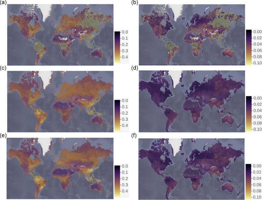
1712                                                                    M. Guevara et al.: Gap-free global annual soil moisture

1   Introduction                                                     datasets (e.g., Soil Moisture Active Passive (Al-Yaari et al.,
                                                                     2019).
                                                                        Across large areas of the world, the ESA-CCI soil mois-
Soil moisture data are essential for scientific inquiry in a vari-   ture data have been validated and calibrated against in situ
ety of research areas. These data enable scientists to charac-       soil moisture measurements (Al-Yaari et al., 2019; Dorigo
terize hydrological patterns (Greve and Seneviratne, 2015),          et al., 2011a). In addition, there are continuing efforts to
quantify the influence of soil moisture on terrestrial carbon        improve the spatial reliability of the satellite measurements
dynamics (van der Molen et al., 2011), identify trends in            (Gruber et al., 2017), resulting in new dataset versions. How-
global climate variability (Seneviratne et al., 2013), analyze       ever, even the most recent versions of ESA-CCI soil moisture
the response of ecosystems to moisture decline (Zhou et al.,         data (i.e., v4.5 to 5.0) still suffer from a too-coarse-grained
2014), or detect the impact of moisture on models of land–           spatial resolution and substantial spatial gaps in their spatial
atmosphere interactions (May et al., 2016). The integrity of         coverage (Llamas et al., 2020), making the data unsuitable to
current soil moisture data is fundamental for a comprehen-           tackle problems such as quantifying the implications of soil
sive understanding of the global water cycle (Al-Yaari et al.,       moisture in water cycle across fine-grained scales or across
2019).                                                               areas with spatial gaps. Scientists have developed empiri-
   The main sources of soil moisture data are in situ soil           cal and physical modeling approaches for predicting miss-
moisture measurements through monitoring networks such               ing satellite soil moisture data (Peng et al., 2017; Sabaghy
as the International Soil Moisture Network (ISMN; Dorigo             et al., 2020) and for evaluating the errors in soil moisture
et al., 2011a) and satellite soil moisture measurements such         satellite model predictions (Gruber et al., 2020). The spatial
as those provided by the European Space Agency Climate               resolution and coverage of these recent studies are still an
Change Initiative (ESA-CCI; Dorigo et al., 2017; Liu et al.,         emergent challenge due to limited data across large areas of
2011). Both measurement techniques can quantify regional-            the world (e.g., extremely dry, extremely wet, or frozen re-
to-continental global soil moisture patterns and dynamics            gions) as well as the signal excessive noise and saturation
(Gruber et al., 2020).                                               affecting the quality of satellite soil moisture records. Con-
   In situ soil moisture measurements assess soil moisture           sequently, there is a need for developing alternative model-
within specific study sites at specific soil depths (e.g., 0–        ing approaches and their validation methods to fill the gaps
5 cm). These measurements are fine-grained as soil moisture          of the ESA-CCI dataset, improving both the spatial resolu-
sensors have a small and localized footprint, and despite na-        tion and the coverage. Recent soil moisture products across
tional and international networks they are limited in much           Europe and the United States (Bauer-Marschallinger et al.,
of the world (Fig. 1). Collection of in situ soil moisture data      2018, Guevara and Vargas, 2019) reveal the possibility of
across large areas is expensive and time consuming; in many          developing high-spatial-resolution surface soil moisture esti-
cases, logistical challenges such as limited funding for data        mates that complement the coarse spatial granularity of avail-
collection and accessibility of soil moisture monitoring sites       able remote sensing products (e.g., ESA-CCI).
make it impossible.                                                     In this study we tackle the need to increase spatial gran-
   On the other hand, satellite soil moisture measurements           ularity and provide gap-free global soil moisture predic-
collected in the form of microwave radiometry using L band           tions. In doing so, we combine a pattern recognition tech-
(∼ 1.4–1.427 GHz) and C band (∼ 4–8 GHz) are more ef-                nique called kernel-weighted k-nearest neighbors (or k-
fective for larger regional-to-global soil moisture measure-         KNN; Hechenbichler and Schliep, 2004) with the use of
ments (Mohanty et al., 2017). As for most available in situ          independent covariate or prediction factors such as topo-
soil moisture measurements, satellite soil moisture datasets         graphic parameters, bioclimatic features, and soil types. Our
are representative for the first 0–5 cm of soil depth. Unlike        approach enables us to augment both spatial resolution and
the fine-grained in situ measurements, satellite soil moisture       coverage in the ESA-CCI dataset despite limited data in large
datasets are available at the global scale in coarse-grained         areas of the world.
grids with spatial resolution ranging between 9 and 25 km               k-KNN is a machine learning (ML) algorithm that has
(Senanayake et al., 2019) and at the regional scale (e.g.,           several benefits for predicting satellite soil moisture at the
the European continent) with a spatial resolution of 3 km            global scale. First of all, k-KNN accounts for non-linearities
grids (Naz et al., 2020). A well-known satellite soil moisture       (e.g., local and regionally specific data patterns). Soil mois-
dataset is collected by ESA-CCI. The ESA-CCI dataset con-            ture data (as a dependent variable) can be predicted as a func-
tains more than 40 years of satellite soil moisture global grids     tion of the spatial variability of environmental data (indepen-
(from 1978 to 2019) with a spatial resolution of ∼ 27 km (Liu        dent variables) with different spatial resolution and coverage
et al., 2011; Chung et al., 2018). This soil moisture dataset        (Peng et al., 2017; Guevara and Vargas, 2019; Llamas et al.,
is a synthesis from multiple soil moisture sources and has           2020). k-KNN can take advantage of the spatial autocorre-
been applied in long-term ecological and hydrological stud-          lation of training data such as the relation between variance
ies (Dorigo et al., 2017). The dataset covers a longer period        and distance between soil moisture observations (Llamas et
of time compared with other satellite-derived soil moisture          al., 2020; Oliver and Webster, 2015) and use it as ancillary

Earth Syst. Sci. Data, 13, 1711–1735, 2021                                           https://doi.org/10.5194/essd-13-1711-2021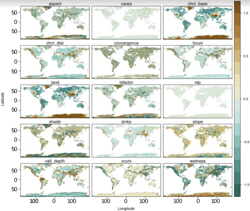
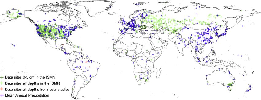
M. Guevara et al.: Gap-free global annual soil moisture                                                                                  1713

Figure 1. Spatial distribution of available data from in situ monitoring sites. This information was only used for validating our soil moisture
predictions. The ISMN (green for all data sites and dark green for sites with available information at 0–5 cm), precipitation records (blue),
and soil moisture additional datasets from previous local studies (red).

information when spatial coordinates (e.g., latitude and lon-             tion contour lines, or digital elevation models) quantitatively
gitude) are considered in the prediction approach (Hengl et               represent topographic variability and are the basis of digi-
al., 2018; Behrens et al., 2018; McBratney et al., 2003). Sec-            tal terrain analysis (i.e., geomorphometry). The topographic
ond, k-KNN can use kernel functions to weight the neighbors               wetness index is a terrain parameter that characterizes areas
according to their distances. Finally, by including spatial co-           where soil moisture increases by the effect of overland flow
ordinates in the predictions, k-KNN can consider geograph-                accumulation (Moore et al., 1993). Overland flow and poten-
ical distances. In doing so, it is able to account for local and          tial incoming solar radiation are two important topographic
regional variability in the feature space: each predicted value           drivers of the spatial distribution of soil moisture (Nicolai-
is dependent on a unique combination of k neighbors in the                Shaw et al., 2015), its lags after precipitation events (Mc-
feature space that are weighted using kernel functions that               Coll et al., 2017), and its role as a dominant control of plant
can be different from one place to another (see Sect. 2.2).               productivity (Forkel et al., 2015). Bioclimatic features and
   We use a diverse set of independent covariates or pre-                 soil types account for hydroclimatic and soil variability af-
diction factors such as topographic parameters, bioclimatic               fecting soil moisture. We add bioclimatic features and soil
features, and soil types to augment the prediction of soil                type classes as additional prediction factors to our approach
moisture values with k-KNN. Topographic parameters are                    to determine if information beyond terrain parameters sub-
based on physical principles related to the overall distribu-             stantially improves soil moisture predictions. To validate our
tion of surface water across the landscape (Western et al.,               dataset, we use independent in situ information (i.e., annual
2002; Moeslund et al., 2013; Mason et al., 2016). We gener-               soil moisture measurements) from local studies (n = 8 sta-
ate the topographic parameters from digital terrain analysis.             tions; Vargas, 2012; Saleska et al., 2013), from the ISMN
Digital terrain analysis involves calculations of land surface            (n = 2185 stations), and from precipitation records across the
characteristics that depend on topography (e.g., terrain slope            world (n = 171 stations, including tropical areas poorly rep-
and aspect; Wilson, 2012). The impact of terrain parameters               resented in the ISMN).
on spatial variability of satellite soil moisture is supported               The contributions of this paper are 2-fold: first, we inte-
by previous studies that have provided evidence of a topo-                grate the k-KNN algorithm and prediction factors into a mod-
graphic signal in satellite soil moisture measurements from               eling approach to predict fine-grained, gap-free soil moisture
local (Mason et al., 2016) to continental scales (Guevara and             data with a resolution of 15 km; second, we generate a new
Vargas, 2019). Other studies derive terrain parameters from               dataset that complements the ESA-CCI dataset and is com-
elevation data and use them to predict soil moisture across               posed of soil moisture predictions from our modeling ap-
a gradient of hydrological conditions (Western et al., 2002).             proach. With reference to our first contribution, we study the
Topographic parameters have also been used for soil attribute             effectiveness of k-KNN in downscaling satellite-derived soil
predictions (Moore et al., 1993) and for soil moisture map-               moisture using two prediction factor datasets: a first dataset
ping applications (Florinsky, 2016). All these studies suggest            based only on topographic parameters and a second based on
that topography (represented by multiple terrain parameters)              topographic parameters, bioclimatic features, and soil types.
is a useful predictor of surface soil moisture variability at the         We compare the accuracy of the two types of fine-grained,
global scale. Different types of terrain parameters exist, in-            gap-free soil moisture models obtained using the two predic-
cluding elevation data structures, topographic wetness, over-             tion factor datasets. The comparison allows us to assess the
land flow, and potential incoming solar radiation, among oth-             impact of the individual prediction factors. Specifically, we
ers. Elevation data structures (i.e., point elevation data, eleva-        address the impact of topographic parameters versus biocli-

https://doi.org/10.5194/essd-13-1711-2021                                                  Earth Syst. Sci. Data, 13, 1711–1735, 2021
1714                                                                  M. Guevara et al.: Gap-free global annual soil moisture

matic features and soil types. Previous studies have used a        values (i.e., data not available; NAs) are between years 2003
variety of prediction factors for soil moisture, including veg-    and 2006 (Appendix A, Fig. A1).
etation indexes (from optical imagery), climate information           We generate and test two different datasets of prediction
(Alemohammad et al., 2018), choropleth maps (i.e., land use        factors with a 15 km grid resolution: (a) a dataset of only
and land forms), thermal data, and soil information to im-         digital terrain parameters and (b) a more complex dataset
prove the spatial resolution and coverage of soil moisture         that uses digital terrain parameters, static bioclimatic fea-
gridded datasets (Naz et al., 2020; Peng et al., 2017). In con-    tures, and soil type information. The second dataset allows
trast to past efforts, our solution uses a comprehensive set of    us to differentiate between the impact of terrain parameters
factors for predicting satellite soil moisture data and indepen-   in isolation and the impact of terrain parameters when aug-
dently testing the model with in situ soil moisture data. Our      mented with static bioclimatic features and soil type informa-
approach is computationally less expensive and prevents po-        tion. The values of prediction factors are generated to over-
tential spurious correlations when predicted soil moisture es-     lap with the central coordinates (latitude and longitude) of
timates are compared with climate, vegetation, or soil infor-      the original ESA-CCI soil moisture pixels following previ-
mation. With reference to our second contribution, we gen-         ous research (Guevara and Vargas, 2019).
erate a dataset complementary to the ESA-CCI soil moisture            Digital terrain parameters (described in Fig. 2) are de-
dataset that provides gap-free global mean annual soil mois-       rived from a global digital elevation model using SAGA-GIS
ture predictions for 28 years (1991–2018) across a 15 km grid      (System for Automated Geoscientific Analysis GIS) (Con-
(note that ESA-CCI has a grid of 27 km). Our soil moisture         rad et al., 2015). The source of elevation data is a radar-
dataset can be used for identifying spatial and temporal pat-      based digital elevation model (Becker et al., 2009). This dig-
terns of soil moisture and its contributions to climate and veg-   ital elevation model is provided by Hengl et al. (2017), and
etation feedbacks. The soil moisture predictions, the field soil   we re-sampled it (along with bioclimatic features and soil
moisture validation dataset, and the set of prediction factors     type classes) to a spatial resolution of 15 km grids across
for soil moisture are publicly available (Guevara et al., 2020).   the world. We consider the following terrain parameters:
                                                                   (a) terrain aspect (aspect), (b) specific catchment area (carea),
2     Methodology                                                  (c) channel network base level (chnl base), (d) distance to
                                                                   channel network (chnl dist), (e) flow convergence index (con-
Our prediction approach has four key steps. First, we de-          vergence), (f) horizontal curvature (hcurv), (g) digital eleva-
fine training soil moisture datasets and define two differ-        tion model (land), (h) length–slope factor (lsfactor), (i) rel-
ent datasets of prediction factors with a 15 km global grid        ative slope position (rsp), (j) analytical hillshade (shade),
resolution: a dataset consisting only of terrain parameters        (k) smoothed elevation (sinks), (l) terrain slope (slope),
and a different dataset combining terrain parameters, bio-         (m) valley depth index (vall depth), (n) vertical curvature
climatic features, and soil type classes (Sect. 2.1). Second,      (vcurv), and (o) topographic wetness index (wetness). The
we build prediction models by feeding the prediction factors       parameters are presented in Fig. 2, and a detailed descrip-
and ESA-CCI satellite soil moisture data to the k-KNN algo-        tion and units of the parameters can be found in Guevara and
rithm and using cross-validation for selecting the best mod-       Vargas (2019).
els (Sect. 2.2). Third, we bootstrap the parameters to assess         Static bioclimatic features are extracted from the Food
variances of soil moisture predictions (Sect. 2.3). Last, we       and Agriculture Organization Global Agro-Ecological Zones
validate our best predictions against independent in situ soil     project (FAO, 2013; baseline period: 1961–1990) to account
moisture measurements when they are available (Sect. 2.4).         for hydroclimatic variability. Thus, these static bioclimatic
                                                                   features consist of a spatial database of land mapping units
                                                                   with the following categories: (1) boreal coniferous forest,
2.1    Training datasets and datasets of prediction factors
                                                                   (2) boreal mountain system, (3) boreal tundra woodland, (4)
We generate a training dataset for each analyzed year              polar, (5) subtropical desert, (6) subtropical dry forest, (7)
(n = 28). A training dataset consists of a table with the cen-     subtropical humid forest, (8) subtropical mountain system,
tral coordinates of each pixel in the ESA-CCI dataset and          (9) subtropical steppe, (10) temperate continental forest, (11)
the corresponding satellite-derived soil moisture values for a     temperate desert, (12) temperate mountain system, (13) tem-
given year. We use all available pixels with valid soil mois-      perate oceanic forest, (14) temperate steppe, (15) tropical
ture values reported in the ESA-CCI v4.5 and calculate (for        desert, (16) tropical dry forest, (17) tropical moist decidu-
each pixel) the mean value of all available observations for a     ous forest, (18) tropical mountain system, (19) tropical rain
given year. We do not consider a threshold value (e.g., a min-     forest, and (20) tropical shrubland.
imum number of pixels) to calculate the mean for each pixel           These categories were developed for assessing global land
for a given year. There are large areas in the world (mainly       resources following a methodology has been jointly devel-
in the tropics or deserts) with missing information through-       oped by FAO and the International Institute for Applied Sys-
out an entire year. After identifying the gaps for each year,      tems Analysis (Fischer et al., 2000). Each category is ex-
we observe that the years with the largest number of missing       pressed within independent maps of zeros and ones (absence

Earth Syst. Sci. Data, 13, 1711–1735, 2021                                         https://doi.org/10.5194/essd-13-1711-2021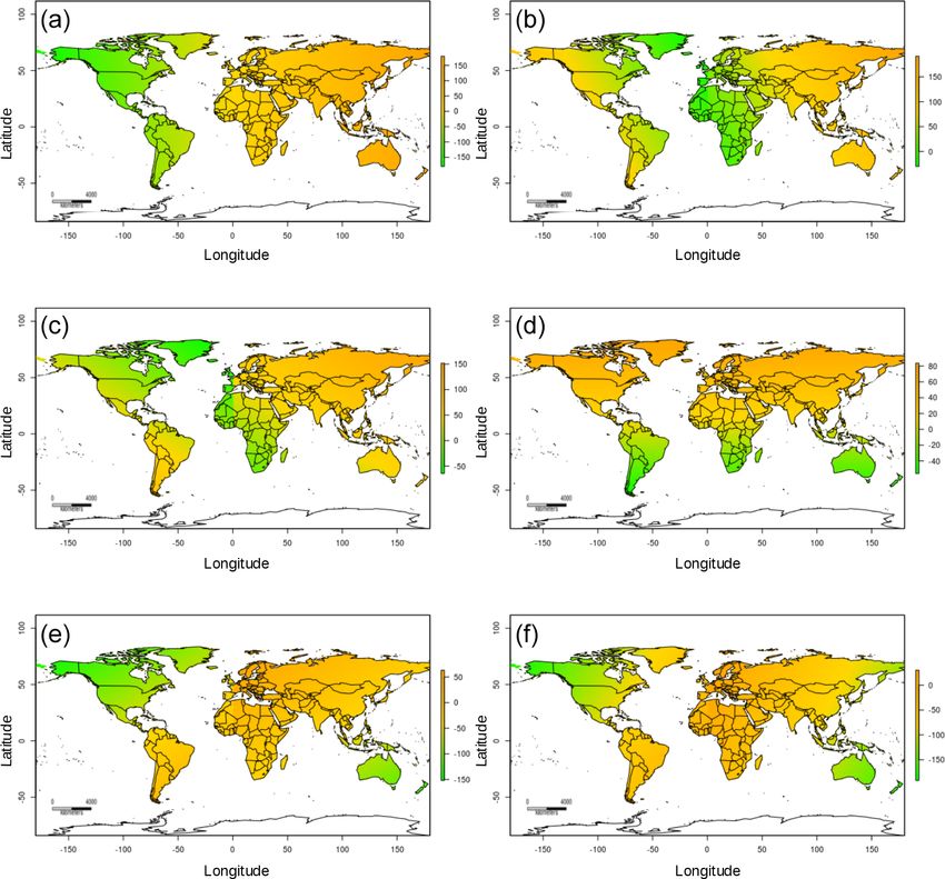
M. Guevara et al.: Gap-free global annual soil moisture                                                                                          1715

Figure 2. Digital terrain parameters used as prediction factors for soil moisture. These parameters are derived from a digital elevation model
using SAGA-GIS. These terrain parameters are standardized by centering their means to zero and a variance unit for visualization purposes.
Legend: (a) terrain aspect (aspect), (b) specific catchment area (carea), (c) channel network base level (chnl base), (d) distance to channel
network (chnl dist), (e) flow convergence index (convergence), (f) horizontal curvature (hcurv), (g) digital elevation model (land), (h) length–
slope factor (lsfactor), (i) relative slope position (rsp), (j) analytical hillshade (shade), (k) smoothed elevation (sinks), (l) terrain slope (slope),
(m) valley depth index (vall depth), (n) vertical curvature (vcurv), and (o) topographic wetness index (wetness). For a detailed description
and units of these parameters see Guevara and Vargas (2019).

and presence, respectively, at each pixel), and this informa-                  extract the values to the corresponding locations of the ESA-
tion is considered as an independent quantitative predictor.                   CCI pixels. By overlapping the original ESA-CCI dataset
   As soil type information, we include soil water retention                   with one of the two prediction factor datasets and extracting
capacity classes (1: 150 mm water per meter of the soil unit;                  the prediction factor values for the ESA-CCI pixel centers,
2: 125 mm; 3: 100 mm; 4: 75 mm; 5: 50 mm; 6: 15 mm; 7:                         we generate two augmented ESA-CCI datasets. A similar
0 mm) from the Regridded Harmonized World Soil Database                        method was initially used for the conterminous United States
v1.2 (Wieder et al., 2014) to account for soil type variability                (Guevara and Vargas, 2019), and here we extend the method
in our prediction framework. In this soil type map the dis-                    to the entire world. In our mapping, we leverage observa-
tance between the above-mentioned water retention classes                      tions from other work outlining the positive impact of spatial
is known (e.g., from high to low every 25 mm of water), and                    structure (e.g., spatial distances and autocorrelation) on soil
it can be considered a quantitative predictor.                                 attribute predictions (e.g., soil moisture) (see spatial coordi-
   For each pixel with available soil moisture values in the                   nate maps in Fig. A1) (Llamas et al., 2020; Møller et al.,
ESA-CCI dataset, we augment the spatial coordinates (i.e.,                     2020; Hengl et al., 2018; Behrens et al., 2018; McBratney et
latitude and longitude) and soil moisture value by adding the                  al., 2003; Oliver and Webster, 2015). We include spatial co-
tuple of the 15 terrain parameters for the first dataset and the               ordinates in our modeling framework (described in Sect. 2.2)
tuple of the 15 terrain parameters, the 19 bioclimatic features,               to account for the spatial structure of the ESA-CCI train-
and the soil type classes for the second dataset. The pixels                   ing data. To this end, we use spatial coordinates at multiple
without soil moisture values become our prediction targets.                    oblique angles as suggested by recent work (Møller et al.,
Because the prediction factor datasets have a 15 km resolu-                    2020, Appendix A, Fig. A2). This preprocessing is done us-
tion while the ESA-CCI soil moisture pixels have a 27 km                       ing open-source R software functionalities for geographical
resolution, we preprocess each prediction factor dataset to                    information systems (R Core Team, 2020; Hijmans, 2019).

https://doi.org/10.5194/essd-13-1711-2021                                                       Earth Syst. Sci. Data, 13, 1711–1735, 2021
1716                                                                    M. Guevara et al.: Gap-free global annual soil moisture

2.2    Building prediction models                                    quires us to randomly create multiple independent training
                                                                     and testing datasets. Training and testing datasets generated
To build prediction models of the soil moisture at a finer           from one of our augmented ESA-CCI datasets are disjoined;
spatial resolution (15 km) than the original ESA-CCI dataset         training data are used for building the models, and testing
(27 km), we use the kernel-based method for pattern recog-           data are used only for quantifying model residuals and eval-
nition known as k-KNN (Hechenbichler and Schliep, 2004).             uating soil moisture predictions.
We build one model per year (n = 28 models). We observe                 As our cross-validation indicators (i.e., information crite-
that the relationships among spatial coordinates, soil mois-         ria about prediction), we use the Pearson correlation coeffi-
ture values, terrain parameters, bioclimatic classes, and soil       cient (r) and the root mean squared error (RMSE) for each
types are not linear. For example, south slope areas tend to         one of the prediction models. For each year we select the
be dryer than north slopes areas. Moreover, there is a con-          model whose combination of k and kernel function has the
trasting feedback of soil moisture and precipitation between         highest r and lowest RMSE. We use the model to predict an-
humid and dry areas (e.g., between the eastern and western           nual mean global soil moisture across 15 km global grids.
United States; Tuttle and Salvucci, 2016). We use k-KNN
because it allows us to account for the non-linear feedback          2.3   Assessing variances of model predictions
while providing a simple and fast prediction solution.
   The k-KNN algorithm has two main settings: (a) the pa-            We study three sources of modeling variance. First, we assess
rameter k that determines the number of neighbors from               the sensitivity of the prediction models to variations in avail-
which information is considered for prediction and (b) a ker-        able training data over the entire world. Second, we assess
nel function that converts distances among neighbors into            the relevance of the spatial coordinates and different predic-
weights, so the farther the neighbor, the smaller the weight         tion factors by rebuilding the models using the k-KNN al-
it will be assigned. We consider k neighbors with k ranging          gorithm with and without each prediction factor, once again
from 2 to 50 soil moisture pixels and with close spatial co-         over the entire world. Third, we assess the effectiveness of
ordinates and similar prediction factors. In the case of the         the k-KNN algorithm across selected areas of the world with
first prediction factor dataset (i.e., only digital terrain param-   fewer data available for training the prediction models and
eters), distances among neighbors are computed among spa-            with different environmental and climate gradients.
tial coordinates and terrain parameters; in the case of the sec-        To assess the sensitivity of the prediction models to varia-
ond dataset (i.e., digital terrain parameters, static bioclimatic    tions in training data, we compute the variance of our soil
features, and soil type classes), distances among neighbors          moisture predictions as surrogates of model-based uncer-
are computed among spatial coordinates, terrain parameters,          tainty. We rebuild the prediction models setting the k-KNN
static bioclimatic features, and soil type classes. The simi-        algorithm to use different random subsets of available pix-
larity among neighbors is measured with the Minkowski dis-           els (n = 1000) and 10-fold repeated cross-validation (n = 10)
tance (i.e., the statistical average of the neighbors’ value dif-    to quantify the variance of soil moisture predictions. This
ference). We consider six different kernel functions (i.e., rect-    model variance enables us to identify geographical areas with
angular, triangular, Epanechnikov, Gaussian, rank, and opti-         high or low sensitivity of prediction models to random vari-
mal).                                                                ations in training data.
   Using the two augmented ESA-CCI datasets obtained by                 To assess the relevance of the different prediction factors,
overlapping the original ESA-CCI dataset with one of the             we use the r and RMSE of modeling with all prediction fac-
two prediction factor datasets and extracting the prediction         tors as a reference, and we compare the r and RMSE with
factor values for the ESA-CCI pixel centers (from Sect. 2.1),        the r and RMSE values of modeling without each one of
we generate two sets of 28 prediction models, one for each of        the prediction factors. We test the sensitivity of the spatial
the 28 years (i.e., 1991–2018) in the ESA-CCI soil moisture          coordinates and each prediction factor (i.e., terrain parame-
dataset (v4.5). We feed the augmented ESA-CCI datasets               ters, bioclimatic features, and soil type classes) by systemat-
into the k-KNN algorithm and search for the most effec-              ically leaving out one prediction factor at a time and repeat-
tive k neighbors’ values and kernel functions. To this end,          ing our k-KNN algorithm and its respective cross-validation.
we use 10-fold cross-validation to select the values of the k        This process is repeated 10 times for each prediction factor
neighbors among the 48 possible values (i.e., k ranged from          to capture a variance estimate. This empirical validation ap-
2 to 50) and the kernel function from these six kernel func-         proach provides empirical insights of the relative importance
tions (i.e., rectangular, triangular, Epanechnikov, Gaussian,        of prediction factors for the k-KNN algorithm predicting soil
rank, and optimal). We use cross-validation as a re-sampling         moisture at the global scale.
technique because it can prevent overfitting in ML methods              To assess the effectiveness of the k-KNN algorithm across
such as k-KNN and can generate multiple sets of indepen-             specific areas of the world, we first test the k-KNN algorithm
dent model residuals to evaluate the stability of prediction         in tropical areas (Appendix A, Fig. A3) with low availabil-
outcomes. The use of cross-validation for searching for the          ity of data to train prediction models (e.g., greater distances
most effective k neighbors’ values and kernel function re-           between k neighbors) and under homogeneous environmen-

Earth Syst. Sci. Data, 13, 1711–1735, 2021                                           https://doi.org/10.5194/essd-13-1711-2021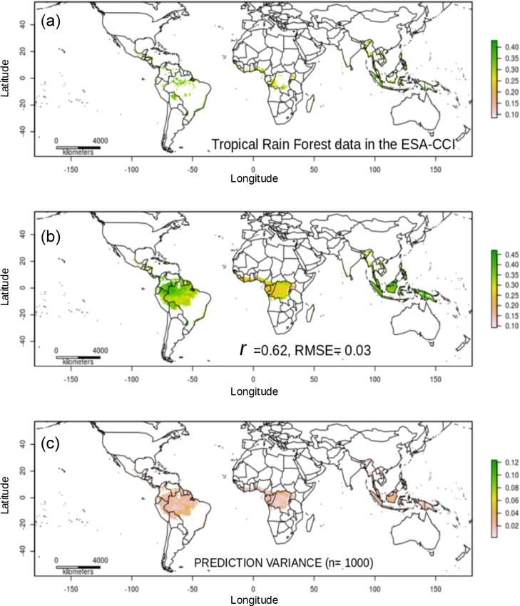
M. Guevara et al.: Gap-free global annual soil moisture                                                                       1717

tal and climate conditions (e.g., higher water content above        ative purposes between the ESA-CCI and our soil moisture
ground than below ground). We extract the limits of tropical        predictions.
areas from the Global Agro-Ecological Zones project (FAO,              We highlight that any potential bias associated with the
2013; baseline period: 1961–1990; described in Sect. 2.1).          data in our augmented ISMN dataset (e.g., stations with low
Second, we test the k-KNN algorithm using only the avail-           number of records) has potentially the same impact on the
able ESA-CCI data across countries with large heterogenous          validation results of the three datasets (ESA-CCI and our two
environmental and climate gradients, such as Canada, Aus-           prediction datasets). In other words, we assume biases are
tralia, and Mexico. We generate new training, testing, and          randomly distributed across all observations, and thus they
prediction factor datasets for these countries using geopo-         are not accounted for in the outcome of our comparisons.
litical limits provided by the Global Administrative Areas          We summarize the validation results in a target diagram to il-
(GADM, 2021). We use the resulting model predictions to             lustrate the accuracy of our soil moisture predictions. The
explore modeling consistency in terms of r and RMSE values          target diagram (presented in Appendix A, Fig. A4; Jolliff
across the selected areas and to visualize spatial patterns be-     et al., 2009) shows the relation between the variance and
tween the ESA-CCI soil moisture dataset and our soil mois-          magnitude of errors (i.e., unbiased root mean squared error,
ture predictions.                                                   or ubRMSE) (a) between the ESA-CCI and the augmented
                                                                    ISMN dataset and (b) between our predictions and the aug-
2.4   Validation against independent in situ data
                                                                    mented ISMN dataset.
                                                                       To compare trends in soil moisture over time for areas for
We validate the ESA-CCI dataset and our predictions against         which we have in situ data, we perform a non-parametric
in situ soil moisture data reported in ISMN for each year.          (median-based) trend detection test (i.e., Theil–Sen estima-
Additionally, we compare soil moisture trends (i.e., changes        tor) to compare soil moisture trends at the locations of the
in soil moisture over time) by comparing either in situ soil        augmented ISMN dataset. This trend detection is done by
moisture or the ESA-CCI with our predictions.                       calculating the median value of the slopes and intercepts of
   We first augment the original ISMN (downloaded in Au-            all possible combinations of pairs of points in the relationship
gust of 2019) from the datasets with information from eight         of soil moisture (response) and time (explanatory variable).
stations with in situ soil moisture data from literature reviews    This resulting median slope and intercept estimates are unbi-
that are distributed in open-access data repositories: one sta-     ased and resistant to outliers (Kunsch, 1989).
tion was deployed in a tropical forest of Mexico with data             For those areas in which the ISMN dataset has multiple
from 2006 to 2008 (Vargas, 2012), and seven stations across         gaps, we rely on the ESA-CCI and our prediction datasets
Brazil’s tropical forests with data from 1999 to 2006 (Saleska      to generate a map of soil moisture trends. To this end, we
et al., 2013).                                                      apply a pixel-wise trend detection test to the ESA-CCI and
   To perform the validation, we compute yearly means at            prediction datasets to search for possible breakpoints (i.e.,
every available location of the ISMN dataset. Then, we or-          significant changes in soil moisture over time). We consider
ganize for further comparisons these yearly means with the          two regression parameters (i.e., slopes and intercepts) before
yearly means of the combined ESA-CCI (v4.5) soil mois-              and after any possible breakpoint to detect trends; in all the
ture grids and our soil moisture predictions. Consequently,         tests, a minimum of 4 years is required between breakpoints
further analyses are consistent in space (i.e., locations from      for detecting trends. To provide our study with robust trend
the ISMN and corresponding pixels in the ESA-CCI (v4.5)             detection estimates, we do not consider segments between
and our predictions) and time (1991–2018). We first calcu-          breakpoints with fewer than eight observations. (Forkel et al.,
late the yearly means using all available soil moisture values      2013, 2015).
per site in the ISMN (n = 2185 stations), and then we ex-
tract the sites containing information of soil moisture for the
0–5 cm for further analyses (n = 987 stations, 1996–2016).          3   Results
   To complement our validation strategy, we perform an ad-
ditional independent validation against in situ records of an-      In our assessment of the results, we first discuss the statis-
nual precipitation (n = 171 stations). This information was         tical description of the observed and modeled soil moisture
extracted from the global soil respiration database (Bond-          datasets (Sect. 3.1). Second, we present the sensitivity of the
Lamberty and Thomson, 2018) and represented the years               prediction models and the way they are generated to vari-
2008 to 2018. Soil moisture and precipitation are closely re-       ations in available datasets (Sect. 3.2). Third, we measure
lated variables (McColl et al., 2017), and previous work has        the relevance of the different prediction factors by rebuild-
recommended the use of soil-moisture-related information to         ing the models using the k-KNN algorithm with and with-
validate soil moisture predictions in the absence of in situ        out one prediction factor at the time over the entire world
soil moisture information (Gruber et al., 2020). The purpose        (Sect. 3.3). Finally, we summarize results on soil moisture
of including precipitation datasets is to enrich the spatial rep-   for models that are trained in regions for which augmented
resentation of soil-moisture-related information for compar-        ISMN datasets exist (Sect. 3.4) and results on soil moisture

https://doi.org/10.5194/essd-13-1711-2021                                          Earth Syst. Sci. Data, 13, 1711–1735, 2021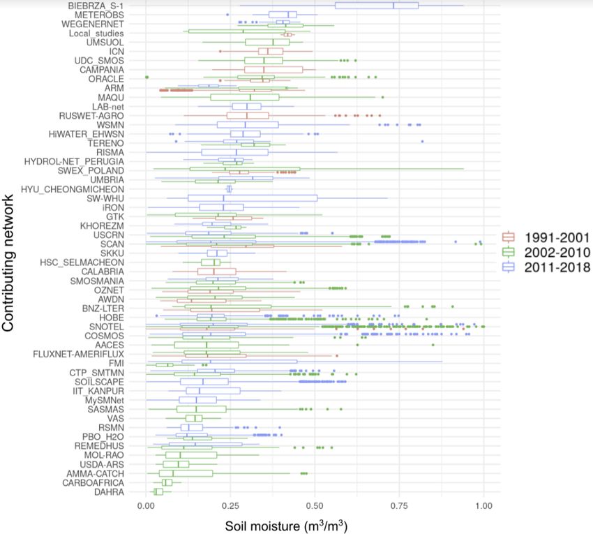
1718                                                                 M. Guevara et al.: Gap-free global annual soil moisture

for models that are trained in regions for which augmented
ISMN datasets do not exist, and thus we use either ESA-CCI
or our predictions as alternative datasets (Sect. 3.5).

3.1    Descriptive statistics

We first assess the statistical distributions of the observed
ESA-CCI dataset, our soil moisture model predictions us-
ing the k-KNN algorithm, and the augmented ISMN dataset
(Fig. 3). Comparing the statistical distribution between ob-
served datasets (i.e., ESE-CCI and ISMN datasets) and our
modeled soil moisture datasets allows us to identify if mod-
eled soil moisture falls within the expected range of observed
soil moisture values. The statistical distribution among dif-
ferent soil moisture datasets can be compared in terms of         Figure 3. Statistical distribution of the ESA-CCI soil moisture
differences in the mean and standard deviation. We present        dataset (red), the predictions of soil moisture using the k-KNN al-
the mean and standard deviation of the ESA-CCI dataset, our       gorithm (gray and green), and the augmented ISMN dataset (black).
modeled soil moisture predictions, and the augmented ISMN         The lines represent the values of each dataset at the locations of all
dataset only at locations (latitude and longitude) where all      existing datasets (locations reported in the augmented ISMN).
datasets have an observation or a prediction. We also restrain
the period of time for our comparisons between 1991 and
2016, which is the period of time with higher consistency of      of data). We repeat the same process for each year, leaving
data availability for both the ESA-CCI dataset and the aug-       out each one of the prediction factors at the time, and assess
mented ISMN dataset.                                              the prediction sensitivity for different datasets as explained
   When comparing the statistical distribution of the soil        in Sect. 2.3. We compute the r and RMSE between obser-
moisture datasets, we observe that the ESA-CCI dataset            vation and model prediction datasets. Our observations are
has mean soil moisture values of 0.29 m3 m−3 and a stan-          soil moisture values from the ESA-CCI dataset and from the
dard deviation of 0.09 m3 m−3 . The modeled soil moisture         augmented ISMN as generated in Sect. 2.4. Our prediction
predictions based only on digital terrain parameters have         factors datasets (defined in Sect. 2.1) are the basis to generate
mean soil moisture values of 0.24 m3 m−3 and a standard           (a) the soil moisture predictions based on terrain parameters
deviation of 0.05 m3 m−3 . Modeled soil moisture predic-          only and (b) the soil moisture predictions based on terrain
tions based on digital terrain parameters, bioclimatic fea-       parameters, bioclimatic features, and soil type classes.
tures, and soil type classes show the mean soil moisture value       We first report results for the entire world using ESA-
is 0.24 m3 m−3 and standard deviation is 0.05 m3 m−3 . The        CCI as a training dataset for building prediction models
augmented ISMN dataset shows a larger range of soil mois-         and repeated cross-validation for assessing the accuracy of
ture values (Fig. 3) when comparing all datasets: the dataset     the model predictions (described in Sect. 2.2). The cross-
values show a mean of 0.25 m3 m−3 and a standard deviation        validated r of soil moisture predictions based on digital ter-
of 0.07 m3 m−3 . We have two key observations. First, we ob-      rain parameters only ranges from 0.69 to 0.81 across years
serve a consistent statistical distribution when comparing the    (1978–2019). The RMSE ranges from 0.03 to 0.04 m3 m−3 .
statistical distribution of the augmented ISMN with the sta-      The soil moisture predictions based on terrain parameters,
tistical distribution of the ESA-CCI dataset (Fig. 3). Second,    bioclimatic features, and soil type classes have a slightly
and more importantly, the mean and standard deviation of our      higher correlation between observed and predicted soil mois-
modeled soil moisture predictions based on terrain parame-        ture values (ranging between 0.78 and 0.85) and slightly
ters only and based on terrain parameters, bioclimatic fea-       lower RMSE values (ranging from 0.02 to 0.04 m3 m−3 ).
tures, and soil type classes as prediction factors show similar   Note that each soil moisture prediction contains a cross-
agreement with the means and standard deviations of both          validation accuracy report (see Sect. 5). The small variations
ESA-CCI and augmented ISMN datasets.                              of r and RMSE indicate a reliable prediction capacity of our
                                                                  models.
3.2    Prediction sensitivity for different datasets
                                                                     For the entire world once again, we assess the sensitiv-
                                                                  ity of our predictions (described in Sect. 2.3) in terms of
We evaluate r and RMSE for 12 040 cross-validated soil            the models’ prediction variance, which ranges from < 0.001
moisture models. The number of models is defined as fol-          to 0.18 m3 m−3 . This prediction variance is higher in areas
lows. For each year (n = 28) we build a model with all pre-       with lower availability of training data from the ESA-CCI
diction factors (n = 42) and assess the variance of 10 model      (e.g., across the tropical areas and coastal areas). These vari-
replicas based on different random data subsets (n − 10 %         ances also serve as surrogates for uncertainty; each file con-

Earth Syst. Sci. Data, 13, 1711–1735, 2021                                          https://doi.org/10.5194/essd-13-1711-2021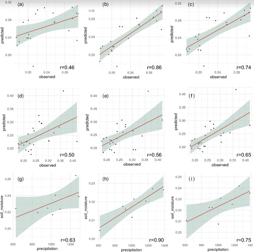
M. Guevara et al.: Gap-free global annual soil moisture                                                                      1719

taining a soil moisture prediction model includes a file with      3.3   Relevance of the different prediction factors
a soil moisture prediction variance (see Sect. 5). For exam-
ple, for the year 2018 (Fig. 4), soil moisture predictions vary
between ∼ 0.001 and ∼ 0.45 m3 m−3 , while the prediction           Across the entire world, we assess the relevance of the dif-
variances range from ∼ 0.001 to 0.14 m3 m−3 , indicating a         ferent prediction factors defined in Sect. 2.1 (i.e., prediction
broader variability around the predicted values. Larger pre-       factors from terrain parameters, bioclimatic features, and soil
diction variances are the combined result of both the higher       type classes) by rebuilding the prediction models using the
possible values of soil moisture and the limited sample size       k-KNN algorithm and removing one prediction factor at a
within the ESA-CCI to train the prediction models, such as         time. By systematically removing one prediction factor at
in tropical areas dominated by dense vegetation.                   a time and using repeated 10-fold cross-validation (n = 10),
   We provide an example of the sensitivity of our models          we can measure the prediction factor impact on the accuracy
across tropical areas with low availability of data for train-     of each model generated for each year using the k-KNN algo-
ing the models as described in Sect. 2.3. For tropical areas of    rithm (Fig. 6). To this end, we compare the cross-validation
the world with limited information in the ESA-CCI datasets,        results (r and RMSE values) of each new model against a
the cross-validated results of the model predictions showed        reference model that we build by using all prediction fac-
r values around 0.62 and RMSE values around 0.03 m3 m−3            tors. Each soil moisture prediction using all prediction fac-
using terrain parameters and soil type classes (Fig. A3). We       tors for each year is accompanied by a reference accuracy
find that the model predictions based only on the limited          report containing the cross-validation results (see Sect. 5).
ESA-CCI soil moisture information available across tropi-          We sort the relevance of prediction factors based on the im-
cal areas (Fig. A3) show a similar prediction variance to          pact of their absence on the cross-validation results (r and
the model predictions for the entire world, with values from       RMSE values), compared with the reference models (using
< 0.001 to < 0.12 m3 m−3 (Fig. A3). These result support the       all prediction factors) across each year. Specifically, for each
effectiveness of our approach across areas with lower avail-       year (1991–2018) and for each factor that is removed at the
ability of information to train the k-KNN algorithm.               time (42 factors), we repeat the cross-validation 10 times as
   We additionally assess the sensitivity of the model pre-        explained in Sect. 2.2 and compute the mean accuracy. For
dictions across areas of the world with heterogeneous en-          each factor, we count the number of times when the absence
vironmental and climate gradients (i.e., geographical extent       of that factor causes a higher r and a lower RMSE compared
of countries such as Mexico, Canada, and Australia), gen-          with the mean accuracy of the reference model generated for
erated as described in Sect. 2.3. The ESA-CCI has rela-            each of the 28 years. Across the years we count the number
tively better spatial coverage across these countries (Fig. 5)     of positive and negative impacts and show the proportion of
compared with tropical areas (Fig. A3) but still has a lower       times (or impact rate) when the absence of each prediction
amount of training data compared with models generated for         factor results in a higher accuracy (i.e., higher r and lower
the entire world. Comparing our soil moisture predictions          RMSE) versus the proportion of times when the absence re-
across 15 km grids with the original ESA-CCI soil moisture         sults in a lower accuracy (i.e., lower r and higher RMSE)
dataset at 27 km grids (Fig. 8) for these areas, we observe that   (Fig. 6).
our soil moisture predictions have consistently higher maxi-          We sort the relevance of prediction factors based on the
mum values (> 0.04 m3 m−3 ) than the original ESA-CCI soil         impact of their absence on the cross-validation results (r and
moisture dataset (< 0.4 m3 m−3 ) (Fig. 5). We observe consis-      RMSE values), compared with the reference models (using
tent modeling accuracy across these countries and across the       all prediction factors) across each year: for r (Fig. 6a) a neg-
entire world (in all cases r values > 0.6 and RMSE values          ative impact rate of a factor means that the model tends to
around 0.04 m3 m−3 ).                                              improve in accuracy (in terms of higher r) when including
   The last two sets of results for tropical areas with low        that factor, and vice versa a positive impact means that the
availability of data and areas of the world with heteroge-         correlation increased when the factor is removed. In contrast,
neous environmental and climate gradients support the ef-          for RMSE (Fig. 6b) a positive impact means that the model
fectiveness of our approach across areas exhibiting unfea-         tends to improve accuracy (in terms of lower RMSE) when
sible data collection and heterogeneous data characteristics,      including that factor, and vice versa a negative impact means
respectively. The flexibility of our prediction models to gen-     that the error decreased when the factor is removed.
erate consistent results on a country-specific basis could be         We observe that spatial coordinates in rotated angles rang-
supported by the use of country-specific information (e.g., to-    ing between 17 and 83◦ (Fig. A2) are coordinates with a pos-
pographic, bioclimatic, and soil information) to predict soil      itive impact on r and RMSE results across years (Fig. 6).
moisture with higher spatial resolution (< 15 km grids) in fu-     Considering each year in isolation, we observe that values
ture research.                                                     for r and RMSE are consistent across individual years. In
                                                                   Fig. 7 we present the values for r and RMSE for 2018 as a
                                                                   representative case. In 2018, we observe that spatial coordi-
                                                                   nates rotated in an oblique angle between 33 and 50◦ (vari-

https://doi.org/10.5194/essd-13-1711-2021                                         Earth Syst. Sci. Data, 13, 1711–1735, 2021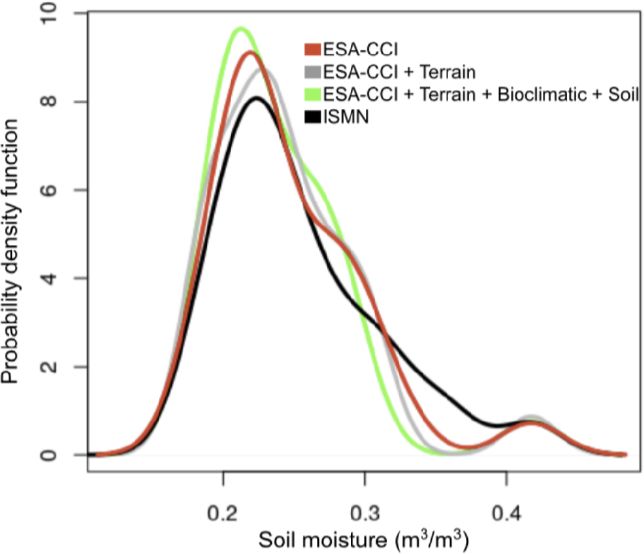
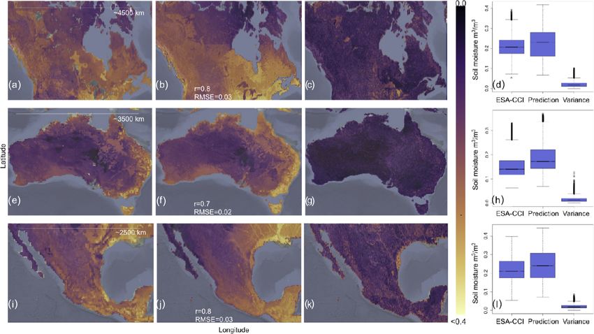
1720                                                                        M. Guevara et al.: Gap-free global annual soil moisture

Figure 4. Soil moisture mean (a) and variance (b) of the ESA-CCI soil moisture product v4.5 between 1991 and 2018. Prediction of soil
moisture (c) and prediction variance (5000 × 5, d) based on topographic terrain parameters. Prediction of soil moisture (e) and prediction
variance (f) based on bioclimatic and soil type classes. Units: m3 m−3 .

Figure 5. Examples of downscaled annual mean soil moisture across specific countries. Prediction of soil moisture, prediction variance,
and training data from the ESA-CCI across Canada (CAN; a–c), and their respective boxplots (showing their statistical distribution) for the
year 2018 (d). Prediction of soil moisture, prediction variance, and training data from the ESA-CCI across Australia (AUS; e–g), and their
respective boxplots for the year 2018 (h). Prediction of soil moisture, prediction variance, and training data from the ESA-CCI across Mexico
(MEX; i–k), and their respective boxplots for the year 2018 (l).

Earth Syst. Sci. Data, 13, 1711–1735, 2021                                                https://doi.org/10.5194/essd-13-1711-2021
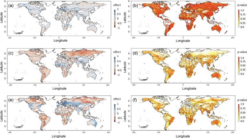
M. Guevara et al.: Gap-free global annual soil moisture                                                                                     1721

Figure 6. Impact of each factor on (a) r and (b) RMSE values across years (1991–2018). The factors with code pi0.00, pi0.17, pi0.33,
pi0.50, pi0.67, and pi0.83 are the spatial coordinates rotated at multiple angles shown in Fig. A2. The rest of the factors are the digital terrain
parameters used to predict the ESA-CCI annual means as they are shown in Fig. 3 and described by Guevara and Vargas (2019): aspect:
terrain aspect; carea: specific catchment area; chnl base: channel network base level; chnl dist: distance to channel network; convergence: flow
convergence index; hcurv: horizontal curvature; land: digital elevation model; lsfactor: length–slope factor; rsp: relative slope position; shade:
analytical hillshade; sinks: smoothed elevation; slope: terrain slope; vall depth: valley depth index; vcurv: vertical curvature; and wetness:
topographic wetness index. The bioclimatic features in (a) tropical, (b) subtropical, (c) temperate, or (e) boreal environments are represented
by binomial variables (0–1). These variables are extracted by the Food and Agriculture Organization Global Agro-Ecological Zones project.
The available water storage capacity variable is represented by continuous classes available thanks to the Regridded Harmonized World Soil
Database.

ables pi0.33 and pi0.50, Fig. A2) have a high impact on r or                Bioclimatic features indicating the presence or absence (0
RMSE values (Fig. 7a).                                                      or 1 binomial variable, respectively) of temperate steppe cli-
   Across all years, we find bioclimatic features have a higher             mate conditions or the presence or absence of tropical shrub-
impact on r or RMSE values, followed by terrain param-                      land climate conditions become top prediction factors for soil
eters and soil classes (Fig. 6), which supports further find-               moisture in this specific year (2018, Fig. 7). The impact of
ings in our validation against in situ soil moisture data con-              terrain parameters has a different impact for predicting soil
tained in the augmented ISMN (in Sect. 3.4). We find that                   moisture variability depending on the average amount of wa-
the use of spatial coordinates has a similar impact on r and                ter reaching the soil (via precipitation and runoff or over-
RMSE values compared with terrain parameters or soil type                   land flow) for each year, which is a process highly dependent
classes (Fig. 6). We observe a slightly higher (but statistically           on bioclimatic conditions. Thus, we can expect to observe
similar) impact of bioclimatic features in cross-validation                 variations in the impact of parameters to predict soil mois-
results compared with terrain parameters (Fig. 6). Biocli-                  ture across specific years (e.g., in extremely dry versus ex-
matic features indicating presence or absence (0 or 1 bino-                 tremely wet years). We provide a variable importance plot
mial variable, respectively) of tropical, subtropical, or tem-              for each year associated with each soil moisture prediction
perate desert (biological and climatological) conditions are                (see Sect. 5).
variables with a high impact on the cross-validation of pre-
diction models. The distance between the base of drainage                   3.4    Soil moisture trained for region for which augmented
network channels and the closest highest point in the ground                       ISMN datasets exist
(before elevation decreases again) (code in Fig. 6: chnl_base)
or the distance of each pixel to the closest drainage net-                  To compare soil moisture values between our predictions and
work channel (code in Fig. 6: chnl_dist) are elevation-derived              the augmented ISMN, we follow two main steps. First, we
(code in Fig. 6: land) terrain parameters with a high impact                assess the r and RMSE values between the ESA-CCI dataset
on r and RMSE across all years. We observe for our example                  and our soil moisture predictions against in situ soil moisture
with the year 2018 that terrain parameters such as chnl_base                using the augmented ISMN. Second, we report changes of
and chnl_dist have a higher impact on r and RMSE values                     soil moisture over time using the augmented ISMN, the ESA-
consistently with our analysis across all years (1991–2018).                CCI, and our soil moisture predictions.

https://doi.org/10.5194/essd-13-1711-2021                                                    Earth Syst. Sci. Data, 13, 1711–1735, 2021
1722                                                                        M. Guevara et al.: Gap-free global annual soil moisture

Figure 7. Impact of each factor on the (a) r and (b) RMSE values for the year 2018. The factors named pi0.00, pi0.17, pi0.33, pi0.50,
pi0.67, and pi0.83 are the spatial coordinates at multiple angles shown in Fig. A2. The digital terrain parameters are shown in Fig. 3 and
described by Guevara and Vargas (2019): aspect: terrain aspect; carea: specific catchment area; chnl base: channel network base level; chnl
dist: distance to channel network; convergence: flow convergence index; hcurv: horizontal curvature; land: digital elevation model; lsfactor:
length–slope factor; rsp: relative slope position; shade: analytical hillshade; sinks: smoothed elevation; slope: terrain slope; vall depth:
valley depth index; vcurv: vertical curvature; and wetness: topographic wetness index. The bioclimatic features divided into (a) tropical,
(b) subtropical, (c) temperate, or (d) boreal environments are represented by binomial variables (0–1). These variables are extracted by the
Food and Agriculture Organization Global Agro-Ecological Zones project. The available water storage capacity variable is represented by
continuous classes available thanks to the Regridded Harmonized World Soil Database.

   Comparing the correlation between in situ and gridded                 provement of our approach over the original ESA-CCI soil
soil moisture datasets, we observe that the correlation of the           moisture dataset.
ESA-CCI (v4.5) with the augmented ISMN across the world                     Across all analyzed years, our global soil moisture pre-
is lower compared to the correlation between soil moisture               dictions represent an improvement as they reduce bias when
predictions based on digital terrain analysis with the ISMN              compared with the ISMN data and in situ precipitation
or soil moisture predictions adding bioclimatic and soil type            records. The variance around the prediction error (e.g., the
classes (Fig. 8).                                                        unbiased RMSE) estimated against the augmented ISMN
   When all available data across all soil depths per site in the        was also lower in our predictions compared with the ESA-
augmented ISMN are considered (n = 2185 stations), the r                 CCI soil moisture dataset (Appendix A, Fig. A4).
values show a mean of 0.50 between the ISMN and the ESA-                    We confirm the effectiveness of the k-KNN algorithm for
CCI, the predictions based on digital terrain parameters show            modeling and predicting soil moisture considering changes
an r value of 0.56, and the predictions including bioclimatic            in soil moisture levels over time (soil moisture trends, Ta-
and soil type classes show an r value of 0.65. Similar levels            ble 1). There is a consistent soil moisture decline over time
of RMSE against the ISMN are found with the models using                 across all soil moisture datasets (i.e., the augmented ISMN
bioclimatic and soil type classes (∼ 0.05 m3 m−3 ) or mod-               and the ESA-CCI datasets; the soil moisture predictions
els using only terrain parameters (∼ 0.05 m3 m−3 ). When                 based on digital terrain analysis; and the predictions using
comparing the ISMN and the ESA-CCI, we observe a mean                    digital terrain analysis, bioclimatic, and soil type classes;
RMSE of 0.09 m3 m−3 . Confirming these results, by restrict-             Table 1) at the specific locations of the augmented ISMN
ing our validation strategy only to the sites with available in-         dataset (Fig. 1). Supporting the effectiveness of the model
formation for the first 0–5 cm of soil depth (n = 987 stations),         predictions, all datasets (observed and modeled soil mois-
we observe correlation values varying from 0.46 for the ESA-             ture) show negative soil moisture trends at locations where
CCI (RMSE =∼ 0.05 m3 m−3 ) to 0.86 using topographic                     all datasets exist (Table 1).
prediction factors (RMSE =∼ 0.03 m3 m−3 ) and 0.74 using
bioclimatic and soil type classes (RMSE =∼ 0.05 m3 m−3 )
as is shown in Fig. 8a–f. The target diagram presented in
Appendix A, Fig. A4, is also useful for visualizing the im-

Earth Syst. Sci. Data, 13, 1711–1735, 2021                                                https://doi.org/10.5194/essd-13-1711-2021
You can also read


