Inverse modelling of carbonyl sulfide: implementation, evaluation and implications for the global budget
←
→
Page content transcription
If your browser does not render page correctly, please read the page content below
Atmos. Chem. Phys., 21, 3507–3529, 2021
https://doi.org/10.5194/acp-21-3507-2021
This work is distributed under
the Creative Commons Attribution 4.0 License.

Inverse modelling of carbonyl sulfide: implementation, evaluation
and implications for the global budget
Jin Ma1 , Linda M. J. Kooijmans2 , Ara Cho2 , Stephen A. Montzka3 , Norbert Glatthor4 , John R. Worden5 , Le Kuai5 ,
Elliot L. Atlas6 , and Maarten C. Krol1,2
1 Institute for Marine and Atmospheric Research, Utrecht University, Utrecht, the Netherlands
2 Meteorology    and Air Quality, Wageningen University & Research, Wageningen, the Netherlands
3 NOAA Global Monitoring Laboratory, National Oceanic and Atmospheric Administration, Boulder, Colorado, USA
4 Institute of Meteorology and Climate Research, Karlsruhe Institute of Technology, Karlsruhe, Germany
5 Jet Propulsion Laboratory, California Institute of Technology, Pasadena, California, USA
6 Rosenstiel School of Marine and Atmospheric Science, University of Miami, Miami, Florida, USA

Correspondence: Jin Ma (j.ma@uu.nl)

Received: 15 June 2020 – Discussion started: 9 July 2020
Revised: 19 January 2021 – Accepted: 21 January 2021 – Published: 8 March 2021

Abstract. Carbonyl sulfide (COS) has the potential to be         layer. Moreover, high latitudes in the Northern Hemisphere
used as a climate diagnostic due to its close coupling to the    require extra COS uptake or reduced emissions. HIPPO
biospheric uptake of CO2 and its role in the formation of        (HIAPER Pole-to-Pole Observations) aircraft observations,
stratospheric aerosol. The current understanding of the COS      NOAA airborne profiles from an ongoing monitoring pro-
budget, however, lacks COS sources, which have previously        gramme and several satellite data sources are used to eval-
been allocated to the tropical ocean. This paper presents a      uate the optimized model results. This evaluation indicates
first attempt at global inverse modelling of COS within the 4-   that COS mole fractions in the free troposphere remain un-
dimensional variational data-assimilation system of the TM5      derestimated after optimization. Assimilation of HIPPO ob-
chemistry transport model (TM5-4DVAR) and a comparison           servations slightly improves this model bias, which implies
of the results with various COS observations. We focus on the    that additional observations are urgently required to constrain
global COS budget, including COS production from its pre-        sources and sinks of COS. We finally find that the biosphere
cursors carbon disulfide (CS2 ) and dimethyl sulfide (DMS).      flux dependency on the surface COS mole fraction (which
To this end, we implemented COS uptake by soil and vege-         was not accounted for in this study) may substantially lower
tation from an updated biosphere model (Simple Biosphere         the fluxes of the SiB4 biosphere model over strong-uptake
Model – SiB4). In the calculation of these fluxes, a fixed at-   regions. Using COS mole fractions from our inversion, the
mospheric mole fraction of 500 pmol mol−1 was assumed.           prior biosphere flux reduces from 1053 to 851 Gg a−1 , which
We also used new inventories for anthropogenic and biomass       is closer to 738 Gg a−1 as was found by Berry et al. (2013). In
burning emissions. The model framework is capable of clos-       planned further studies we will implement this biosphere de-
ing the COS budget by optimizing for missing emissions us-       pendency and additionally assimilate satellite data with the
ing NOAA observations in the period 2000–2012. The ad-           aim of better separating the role of the oceans and the bio-
dition of 432 Gg a−1 (as S equivalents) of COS is required       sphere in the global COS budget.
to obtain a good fit with NOAA observations. This miss-
ing source shows few year-to-year variations but consider-
able seasonal variations. We found that the missing sources
are likely located in the tropical regions, and an overesti-
mated biospheric sink in the tropics cannot be ruled out due
to missing observations in the tropical continental boundary

Published by Copernicus Publications on behalf of the European Geosciences Union.
3508                                                                                  J. Ma et al.: Global inverse modelling of COS

1   Introduction                                                       der to fit the observed seasonal cycle of the COS mole frac-
                                                                       tion, they had to double the terrestrial vegetation uptake es-
Carbonyl sulfide (COS or OCS) is a low abundant trace gas              timated in Kettle et al. (2002), reduce the southern extra-
in the atmosphere with a lifetime of about 2 years and a tro-          tropical ocean source and assume an additional COS source
pospheric mole fraction of about 484 pmol mol−1 (Montzka               of 235 Gg a−1 . Campbell et al. (2008) found that this upward
et al., 2007). COS is regarded as a promising diagnostic               revision could be validated using direct observations from the
tool for constraining photosynthetic gross primary produc-             continental boundary layer from the intensive INTEX-NA
tion (GPP) of CO2 through similarities in their stomatal con-          airborne campaign. Berry et al. (2013) implemented COS
trol (Montzka et al., 2007; Campbell et al., 2017; Berry et al.,       in the global biosphere model SiB3. They inferred that, in
2013; Whelan et al., 2018; Kooijmans et al., 2017, 2019;               order to compensate for updated COS biosphere and soil
Wang et al., 2016). COS also contributes to stratospheric              sinks of 1093 Gg a−1 , there must be additional COS sources
sulfur aerosols, which have a cooling effect on climate and            of 600 Gg a−1 , which were allocated to the ocean. Glatthor
hence mitigate climate warming (Crutzen, 1976; Andreae                 et al. (2015) and Launois et al. (2015) estimated direct COS
and Crutzen, 1997; Brühl et al., 2012; Kremser et al., 2016).          emissions from the ocean as 992 and 813 Gg a−1 , respec-
In recent decades, COS mole fractions in the troposphere               tively, and also Kuai et al. (2015) hinted at underestimated
have remained relatively constant, which implies that sources          COS sources from tropical oceans by optimizing sources us-
and sinks of COS are balanced. Whelan et al. (2018) re-                ing 1 month of COS satellite observations by the Tropo-
viewed the state of current understanding of the global COS            spheric Emission Spectrometer on Aura (TES-Aura). How-
budget and the applications of COS to ecosystem studies of             ever, Lennartz et al. (2017, 2019) used COS measurements in
the carbon cycle. The most pressing challenge currently is to          ocean water to show that the direct oceanic emissions were
reconcile the balance of COS sources and sinks, given the              much lower (130 Gg a−1 ) than top-down studies suggested.
small global atmospheric trends.                                       It is therefore not resolved whether ocean emissions account
   Previous studies show that substantial emissions of COS             for the missing source.
are coming from oceanic, anthropogenic, and biomass burn-                 In this paper, we address several important open questions
ing sources and the largest sinks are uptake by plants and             concerning the COS budget using inverse modelling tech-
soils (Watts, 2000; Kettle et al., 2002; Berry et al., 2013).          niques, employing the TM5-4DVAR modelling system. We
Oceanic emissions are thought to be the largest source of              focus on the closure of the COS budget, the contributions
COS, both directly and indirectly, due to emissions of CS2             of the potential COS precursors CS2 and DMS, and evalua-
and possibly DMS (Lennartz et al., 2017, 2020), which can              tion of the results with aircraft and satellite observations. In
be quickly oxidized to COS in the atmosphere (Sze and                  Sect. 2 we will describe the observations; the implementation
Ko, 1980). There are considerable uncertainties related to             of COS, CS2 and DMS in TM5; and the inverse modelling
this indirect COS source, with reported yields of COS being            system TM5-4DVAR. In Sect. 3, we will analyse the results
(83 ± 8) % from CS2 (Stickel et al., 1993) and (0.7 ± 0.2) %           of various inverse model calculations, which are discussed
from DMS under NOx -free conditions at 298 K (Barnes                   further in Sect. 4.
et al., 1996). Blake et al. (2004) reported anthropogenic
Asian emissions for COS and CS2 , which appear to have
been underestimated by 30 %–100 % due to underestimated                2     Method
coal burning in China (Du et al., 2016). Zumkehr et al. (2018)
                                                                       This study aims to close the gap in the global COS budget
recently presented a new global anthropogenic emission in-
                                                                       by so-called flux inversions. This technique employs atmo-
ventory for COS. The new anthropogenic emission estimates
                                                                       spheric measurements to optimize sources and sinks of trace
are, with 406 Gg a−1 (as S equivalents)1 in 2012, substan-
                                                                       gases such that mismatches between simulations and obser-
tially larger than the previous estimate of 180.5 Gg a−1 by
                                                                       vations are minimized. In Sect. 2.1 the observations used in
Berry et al. (2013). Another recent study (Stinecipher et al.,
                                                                       this study are introduced. Section 2.2 will subsequently de-
2019) concluded that it is unlikely that biomass burning ac-
                                                                       scribe our modelling system, including new emission data
counts for the balance between sources and sinks of COS,
                                                                       sets that have been coupled to the modelling system. The in-
due to the relatively small contribution of biomass burning to
                                                                       verse modelling framework is discussed in Sect. 2.3.
the total emissions ((60 ± 37) Gg a−1 ).
   Suntharalingam et al. (2008) made a first attempt to sim-           2.1     Measurements
ulate the global COS budget using the GEOS-Chem model
and global-scale surface measurements from NOAA. In or-                2.1.1    NOAA flask data

    1 Conventionally, the unit of COS sources or sinks is normally     The NOAA surface flask network provides long-term mea-
written as Gg S a−1 to account for the mass of sulfur. To keep clar-   surements of the COS mole fraction at 14 locations at
ity of the physical unit, we use Gg a−1 throughout the paper but       weekly–monthly frequencies. Most of the stations are lo-
account only for mass of sulfur in COS, CS2 and DMS.                   cated in the Northern Hemisphere (NH), as shown in Fig. 1.

Atmos. Chem. Phys., 21, 3507–3529, 2021                                                   https://doi.org/10.5194/acp-21-3507-2021
J. Ma et al.: Global inverse modelling of COS                                                                                                     3509

Table 1. The split of anthropogenic emissions in the different cate-                    In some numerical experiments, HIPPO data are additionally
gories and between COS and CS2 based on Zumkehr et al. (2018).                          assimilated to investigate their impact on the optimized COS
Note that we used a CS2 -to-COS molar yield of 0.87 and that CS2                        budget. To investigate this impact on the vertical distribution
contains two S atoms. Averages over 2000–2012 are presented.                            of COS, we compared model results to 2008–2011 NOAA
                                                                                        airborne data that are mainly available over North America
  Emission type                     Total     Fraction        Direct       Direct       (Fig. 1). The number of aircraft sites used is 19, and the upper
                                    COS         COS∗           COS          CS2
                                                                                        altitude that was typically reached is 8 km.
                                  Gg a−1              %      Gg a−1      Gg a−1
  Agricultural chemicals             16.9           0.0          0.0         38.9       2.1.3   Satellite data
  Aluminium smelting                 22.2          88.2         19.6          6.0
  Industrial coal                    52.1          99.5         51.8          0.7       Our inverse modelling results are compared to three in-
  Residential coal                   54.0         100.0         54.0          0.0       dependent satellite data sources: TES-Aura, the Atmo-
  Industrial solvents                 5.4           0.0          0.0         12.5       spheric Chemistry Experiment Fourier Transform Spectrom-
  Carbon black                       19.7          26.5          5.2         33.3       eter (ACE-FTS) and the Michelson Interferometer for Pas-
  Titanium dioxide                   39.4          26.5         10.5         66.6
  Pulp & paper                        0.1           3.2          0.0          0.3
                                                                                        sive Atmospheric Sounding (MIPAS). We have selected the
  Rayon yarn                         41.1           0.0          0.0         94.6       period 2008–2011 for the comparison.
  Rayon staple                       77.3           0.0          0.0        177.7          NASA’s TES is both a nadir- and a limb-viewing instru-
  Tyres                              15.1          43.0          6.5         19.8       ment that flies on the Aura satellite, which was launched in
  Total anthropogenic               343.3             –        147.5        450.2       2004 (Beer et al., 2001). TES measures the infrared radia-
∗ The fraction of COS is calculated based on the COS-to-CS emission ratio reported in
                                                          2                             tion emitted from the Earth and atmosphere in a high spec-
Table 1 of Lee and Brimblecombe (2016).
                                                                                        tral resolution for 16 orbits every other day. From these spec-
                                                                                        tra, abundances of tropospheric trace gases are retrieved. The
Although the number of sampling sites is modest, their lo-                              COS product used in this study is described in Kuai et al.
cations cover most latitudinal regions and sample over both                             (2014). The COS retrievals cover the whole vertical column,
land and coastal areas. It is worth noting that there is a lack                         have less than 1◦ of freedom (DOF) and show maximum sen-
of observations in the tropical continental boundary layer.                             sitivity in the 300–500 hPa region. We will therefore focus
The observational error for each sample is relatively small (<                          our comparisons on total COS columns. To account for the
7 pmol mol−1 ); therefore we have taken inter-annual variabil-                          non-uniform vertical sensitivity, we use the averaging ker-
ity in COS from Table 1 in Montzka et al. (2007) to represent                           nel (AK) in the model–satellite comparison. As described in
a fixed observational-error upper limit at each site. In general,                       Kuai et al. (2014), the AK included in the TES data files is
the observational error defined in this way varies between 4–                           defined in log space and should be applied as
10 pmol mol−1 in the NH and between 2–4 pmol mol−1 in the
Southern Hemisphere (SH). This error is used in the inverse                             ln(χ con ) = ln(χ p ) + A[ln(χ m ) − ln(χ p ) + β],         (1)
modelling as will be described in Sect. 2.4.
                                                                                        where χ con , χ p and χ m are the convolved, prior and mod-
2.1.2     HIPPO aircraft and NOAA airborne data                                         elled profiles, respectively, and A is the AK. β is a global
                                                                                        constant bias correction term. In Kuai et al. (2015) a β value
Flask data of the HIAPER Pole-to-Pole Observations                                      of 0.2 was derived using inverse modelling, partly to account
(HIPPO) experiments (Wofsy, 2011; Wofsy et al., 2017) are                               for the missing stratospheric decay in that study. In Sect. 3.4
used to validate the results of the inverse modelling. There                            the modelled profiles are convolved with the TES AK (χ con ),
were five HIPPO campaigns conducted from 2009 to 2011                                   vertically integrated, and compared to the TES columns.
that sampled the COS mole fraction from the North Pole                                     ACE-FTS is a high-spectral-resolution infrared Fourier
to the South Pole and from the lower troposphere up to the                              transform spectroscopy instrument that performs solar occul-
stratosphere. Three different instruments were used to make                             tation measurements, with the aim of sampling stratospheric
measurements of COS during HIPPO. Instrument 2 was used                                 and upper tropospheric profiles of trace gases (Boone et al.,
by NOAA to measure COS, and instrument 1 was calibrated                                 2013). The instrument flies on SCISAT, a Canadian satellite
consistently with the NOAA calibration standard. Results of                             mission for remote sensing of the Earth’s atmosphere that
instrument 3 were scaled to be consistent with those of in-                             was launched in 2003. Its orbit covers tropical, mid-latitude
strument 2, such that results from all three instruments on                             and polar regions. COS is one of the atmospheric trace gases
HIPPO are referenced to the same NOAA scale. The proba-                                 measured by the ACE-FTS instrument (Koo et al., 2017).
bility distribution function of the mole fractions confirms that                        ACE-FTS profiles have been compared to balloon observa-
the three instruments report consistent values, with similar                            tions and have generally shown good agreement, with under-
averages (see Fig. S1). Thus, HIPPO data provide valuable                               estimations smaller than 20 % (Krysztofiak et al., 2015). We
data to check the consistency of the optimized COS budget.                              use product version 3.6, and only observations with a qual-
The flight routes of the five campaigns are shown in Fig. 1.                            ity flag of zero are used. ACE-FTS measures COS within

https://doi.org/10.5194/acp-21-3507-2021                                                                  Atmos. Chem. Phys., 21, 3507–3529, 2021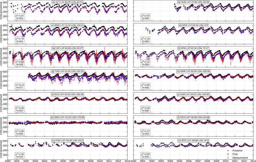
3510                                                                              J. Ma et al.: Global inverse modelling of COS

Figure 1. Geographical locations of the NOAA ground-based observations (shown in boxes), the five HIPPO campaign tracks and the NOAA
profile programme (inset). Note that there are no NOAA surface stations located in Asia, South America or Africa.

0–150 km vertically, but the data quality is only sufficient in       The retrievals of TES, MIPAS and ACE-FTS v3.6 are pro-
the upper troposphere and lower stratosphere (UTLS).                vided on 14, 60 and 150 vertical levels in the atmosphere, re-
   MIPAS is a Fourier transform spectrometer for detection          spectively. We map our modelled COS profiles to these levels
of the radiative emission of various molecules in limb ob-          using a mass-conserving interpolation scheme.
servation mode in the middle and upper atmosphere (Fis-
cher et al., 2008). MIPAS flew on ESA’s Envisat platform            2.1.4    Seasonal decomposition
that operated between 2002–2012. MIPAS delivers global at-
mospheric COS profiles in the upper troposphere and strato-         In Sect. 3.1 we apply a simple seasonal decomposi-
sphere (Glatthor et al., 2015, 2017). Similarly to TES, the         tion method to our calculated exchange fluxes. The sea-
MIPAS data product contains representative AKs and prior            sonal decomposition is performed using the Python module
profiles to facilitate comparison to modelled profiles but not      statsmodels, version 0.10. The time series are decomposed
in log space, since MIPAS COS is evaluated by a linear re-          into trend, seasonality and noise:
trieval:                                                            y(t) = y t (t) + y s (t) + y r (t),                         (3)

χ con = χ p + A[χ m − χ p ],                                (2)     with y(t) being the monthly exchange fluxes and y t , y s and
                                                                    y r the trend, seasonal and residual components, respectively.
where χ m has to be resampled on the MIPAS retrieval grid           2.2     Model description
in advance.
   As for most other gases, the prior profile for MIPAS COS         2.2.1    Anthropogenic emissions
retrievals is a zero profile. Equation (2) thus becomes a sim-
ple multiplication of the AK with the modelled profiles. A          We have implemented the anthropogenic emissions based on
detailed description of the application of MIPAS AKs on             a recent global gridded emission inventory of COS (Camp-
other data sets can be found in Stiller et al. (2012).              bell et al., 2015; Zumkehr et al., 2018). Since we were aim-
   The MIPAS product has been compared to modelled COS              ing to model COS, CS2 and DMS as separated tracers, we
distributions (Glatthor et al., 2015) and ACE-FTS (Glatthor         disentangled the reported COS emissions into COS and CS2
et al., 2017). The latter comparison showed that MIPAS re-          contributions. Here, we applied an assumed yield of 0.87
trieves higher mole fractions around the tropopause com-            (Zumkehr et al., 2018), which means that 1 mol of CS2 yields
pared to ACE-FTS. The MIPAS product has also been com-              0.87 mol of COS. As a precursor of COS, CS2 reacts with
pared to airborne measurements of the HIPPO, ARCTAS and             OH to produce COS and has an atmospheric lifetime of about
INTEX-B campaigns (Supplement of Glatthor et al., 2015).            12 d (Khalil and Rasmussen, 1984). We applied a detailed an-
Finally, MIPAS has been compared to MkIV and SPIRALE                thropogenic emission budget for COS and CS2 from Table 1
profiles (Glatthor et al., 2017).                                   in Lee and Brimblecombe (2016). This allows us to roughly

Atmos. Chem. Phys., 21, 3507–3529, 2021                                                 https://doi.org/10.5194/acp-21-3507-2021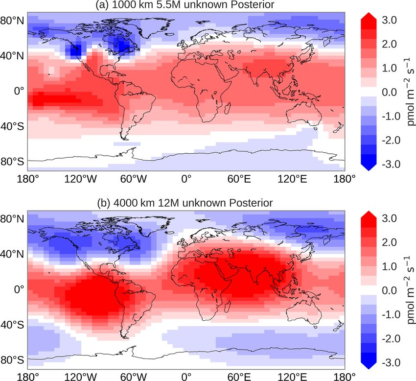
J. Ma et al.: Global inverse modelling of COS                                                                                 3511

estimate the ratio of this budget and hence the direct and indi-   Table 2. Biomass burning emission factors used in converting COS
rect COS anthropogenic emissions. The converted emissions          emissions. EF COS denotes the COS emission factor from dry mass
averaged over the period 2000–2012 are summarized in Ta-           in units of g kg−1 COS per dry mass, and EF CO denotes the CO
ble 1.                                                             emission factor in g kg−1 CO per dry mass. Emission factors were
   The total anthropogenic COS emissions are on aver-              taken from Andreae (2019).
age 343.3 Gg a−1 , split between direct COS emissions of
                                                                                                       EF COS          EF CO
147.5 Gg a−1 and CS2 emissions of 450.2 Gg a−1 . This in-
dicates that CS2 is an important precursor of COS. Figure 2                                          g kg−1 COS      g kg−1 CO
shows time series of COS and CS2 anthropogenic emissions.                                           per dry mass    per dry mass
COS emissions are dominated by industrial and residential            Savanna and grassland              0.038            –
coal sources, while CS2 emissions are dominated by rayon             Tropical forest                    0.078            –
industry and TiO2 production. Moreover, while COS emis-              Temperate forest                   0.035            –
sions remained relatively constant in the 2007–2012 period,          Boreal forest                      0.058            –
CS2 emissions showed an increasing trend.                            Peat fires                         0.110            –
   While Zumkehr et al. (2018) assumed a molar yield of CS2          Agricultural waste burning         0.059            –
to COS of 87 %, other reported yields are (83 ± 8) % (Stickel        Biofuel burning without dung       0.017            83
et al., 1993) and 81 % (Chin and Davis, 1993). We decided            Biofuel burning with dung          0.210            89
to use a yield of 83 % in our modelling, while we used the
reported yield of 87 % to produce the numbers listed in Ta-
ble 1. This implies that we introduce slightly less COS into       2.2.3   Biosphere flux
the atmosphere compared to using the Zumkehr et al. (2018)
data as direct COS emissions. Note that we apply all categor-      Our biosphere fluxes are based on simulations with the Sim-
ical emissions or fluxes with a monthly time resolution. It is     ple Biosphere Model, version 4 (SiB4) (Berry et al., 2013;
also worth noting that the uncertainty in the anthropogenic        Haynes et al., 2019). Currently, soil uptake is scaled to the
inventory is much larger than the uncertainty in molar yield.      CO2 soil respiration term, and the implementation of specific
                                                                   COS soil models (Sun et al., 2015; Ogée et al., 2016) is ongo-
2.2.2   Biomass burning emissions                                  ing. SiB4 was constrained by a prescribed COS mole fraction
                                                                   of 500 pmol mol−1 outside the canopy. This 500 pmol mol−1
We estimated biomass burning emissions based on the
                                                                   is merely a placeholder and probably leads to too large fluxes
widely used GFED V4.1 data set (Randerson et al., 2018)
                                                                   over the active biosphere, where COS mole fractions de-
for six of the seven emission categories listed in Table 2.
                                                                   cline because of strong uptake. This is further discussed in
In converting dry mass burned to COS emissions, we used
                                                                   Sect. 3.5. Meteorological data that are used as forcing for
the updated emission factors reported in Andreae (2019).
                                                                   SiB4 are taken from the Modern-Era Retrospective Analy-
For biofuel use, we base our estimates on the Community
                                                                   sis for Research and Applications (MERRA) and are avail-
Emissions Data System (CEDS) (Hoesly et al., 2018). We
                                                                   able from 1980 onwards (Rienecker et al., 2011). A spin-
calculated COS emissions by first converting CO emissions
                                                                   up of the model was performed for the period 1850–1979
to dry mass burned, which was converted to COS emissions
                                                                   to reach an equilibrium of the carbon pools. As no MERRA
in a second step. Emission factors are listed in Table 2. In
                                                                   data were available for the spin-up period, the climatologi-
this process we made a distinction between biofuel with and
                                                                   cal average of MERRA data over the period 1980–2018 was
without dung. Dung burning is mainly employed in south-
                                                                   used as meteorological input for the spin-up period. A fi-
ern Asia (Fernandes et al., 2007), and we applied the dung
                                                                   nal simulation was performed for 1980–2018 with the actual
emission ratios only in the region 0–40◦ N and 60–100◦ E.
                                                                   MERRA driver data. The 2000–2018 average flux to the bio-
Our biomass burning emissions in the 2000–2012 period are
                                                                   sphere (vegetation plus soil) amounts to −1053 Gg a−1 , in
in the range of 118–154 Gg a−1 (Fig. 2) and similar to the
                                                                   line with estimates of −951 Gg a−1 using SiB3 (Kuai et al.,
emissions used in Berry et al. (2013) (135 Gg a−1 ) and esti-
                                                                   2015; Berry et al., 2013). The spatial and seasonal distribu-
mates reported in Campbell et al. (2015) (116 ± 52 Gg a−1 ).
                                                                   tion of the biosphere uptake is shown in Fig. S3. The up-
The more recent biomass burning estimate from Stinecipher
                                                                   take shows a large seasonal cycle in the NH and large uptake
et al. (2019) based on GFED 1997–2016 data reports global
                                                                   over tropical forests. The biosphere fluxes were deployed on
emissions of 60 ± 37 Gg a−1 . Note, however, that biofuel use
                                                                   a monthly timescale.
is not included in this estimate. The spatial and seasonal dis-
tribution of the biomass burning emissions averaged over the       2.2.4   Ocean emissions
period 2000–2012 is presented in Fig. S2 in the Supplement.
                                                                   Climatological ocean emissions of COS and the COS pre-
                                                                   cursors CS2 and DMS are based on Suntharalingam et al.
                                                                   (2008) and Kettle et al. (2002). Large quantities of COS,

https://doi.org/10.5194/acp-21-3507-2021                                            Atmos. Chem. Phys., 21, 3507–3529, 2021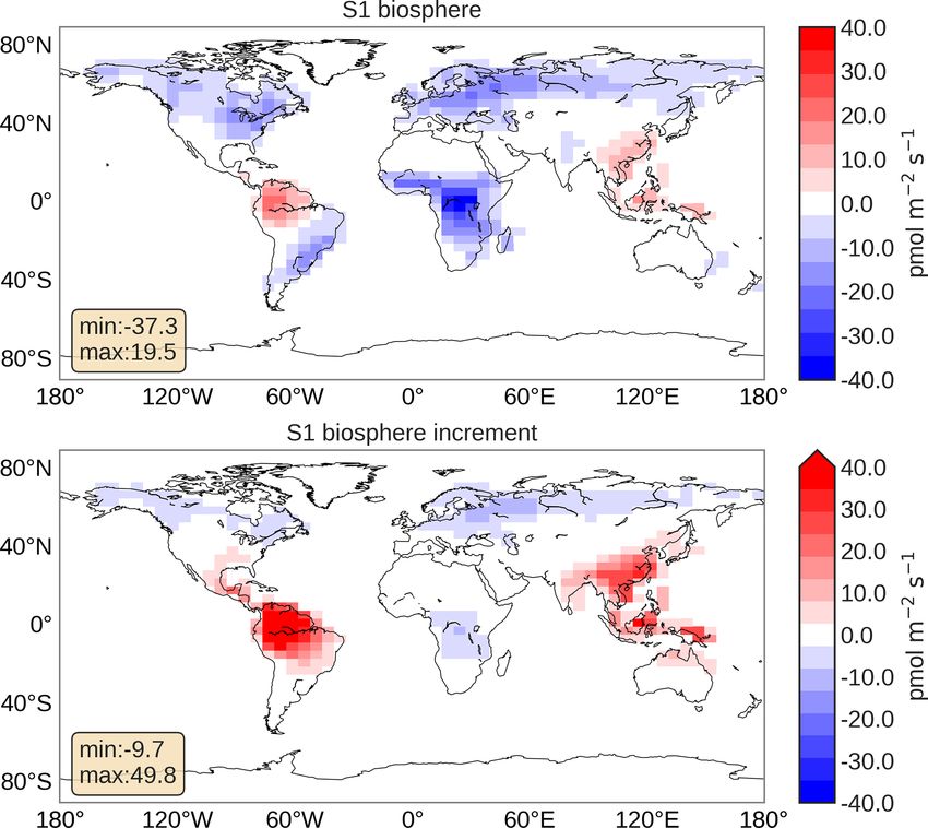
3512                                                                                   J. Ma et al.: Global inverse modelling of COS

Figure 2. Yearly anthropogenic emissions of COS and CS2 as well as COS biomass burning emissions in the period 2000 to 2012. We
disentangled the emissions reported in Zumkehr et al. (2018) into COS and CS2 emissions using their reported yield of 0.87 (see main text).
Biomass burning emissions are calculated based on the GFED V4.1 biomass burning inventory and the CEDS biofuel emission inventory
(see main text).

DMS and CS2 are emitted from open oceans. The estimated                 oceanic emissions as 277 Gg a−1 is substantially smaller than
DMS emissions are about 22 Tg a−1 , and we note that even               the estimate of 813 Gg a−1 by Launois et al. (2015).
if the COS yield from oxidation of DMS is as small as 0.7 %
(Barnes et al., 1996), 156 Gg a−1 COS has already been                  2.3   TM5-4DVAR inverse modelling system
formed. The CS2 direct emissions from oceans are roughly
195 Gg a−1 , yielding 81 Gg a−1 of COS. When the ocean wa-              We have implemented three tracers (COS, CS2 and DMS) in
ter is cold enough, oceans can turn into a sink of COS instead          the inverse modelling framework TM5-4DVAR (Krol et al.,
of a source (Lennartz et al., 2017). Figure S4 shows the spa-           2005, 2008; Meirink et al., 2008). In brief, the TM5 model is
tial distribution of the January and July direct and indirect           used to convert fluxes, collected in state vector x, to observa-
ocean emissions of COS. Note that our estimate of all COS               tions y:
                                                                        y = H ( x ),                                                   (4)

Atmos. Chem. Phys., 21, 3507–3529, 2021                                                    https://doi.org/10.5194/acp-21-3507-2021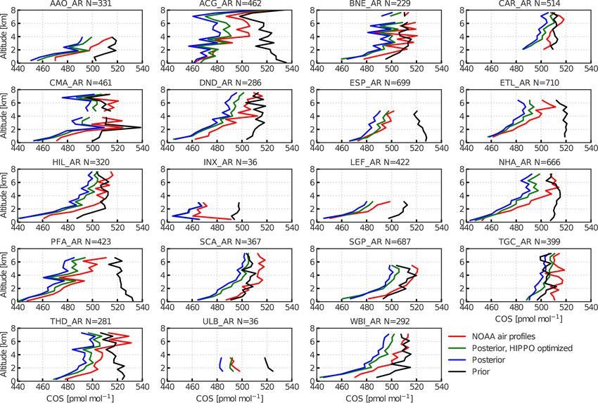
J. Ma et al.: Global inverse modelling of COS                                                                                       3513

Figure 3. Error analysis for NOAA stations. Black error bars represent the time variations in the errors over a 3-year period (2008–2010).
For ALT, SPO and SUM, the flux-related errors are close to zero and not shown. Stations are ordered from the North Pole to the South Pole.

where H represents the global chemistry transport model                of CS2 and DMS to COS. CS2 and DMS are short-lived
TM5. Since the relation between fluxes and observations is             trace gases, with atmospheric lifetimes of approximately 12 d
currently linear, y = H ( x ) can be written as y = H x. In a          (Khalil and Rasmussen, 1984) and 1.2 d (Khan et al., 2016;
flux inversion a cost function is minimized. The cost function         Boucher et al., 2003; Breider et al., 2010), respectively. For
has the following form:                                                CS2 we implemented OH-initiated conversion to COS, while
                                                                       for DMS we simply apply exponential decay with a lifetime
       1
J (x) = (x − x b )T B−1 (x − x b )                                     of 1.2 d. COS itself is also destroyed by OH in the tropo-
       2                                                               sphere and by photolysis in the stratosphere. For OH, we
       1                                                               use monthly varying climatological OH fields (Spivakovsky
      + (y − H x)T R−1 (y − H x),                              (5)
       2                                                               et al., 2000) and apply a correction factor of 0.92 (Naus et al.,
where x b represents the prior state of the fluxes and B and           2019). In summary, the chemistry that is implemented there-
R are the error covariance matrices of the fluxes and obser-           fore consists of the following four reactions:
vations, respectively. B contains the errors assigned to the
fluxes, as well as their correlations in space and time (i.e. B                         r1
                                                                       COS + OH −
                                                                                → products,                                         (R1)
is a non-diagonal matrix). R contains the errors assigned to
                                                                                      j1
(y − H x). These errors are assumed to be uncorrelated and             COS + hν −
                                                                                → products,                                         (R2)
they also include, besides the observational errors, errors re-                        r2
lated to the process of mapping coarse-scale fluxes x to lo-           CS2 + OH −
                                                                                → f1 COS + other products,                          (R3)
calized observations y. The adjoint of the TM5 model (Krol                    r3
                                                                       DMS −
                                                                           → f2 COS + other products,                               (R4)
et al., 2008; Meirink et al., 2008) is used to calculate the gra-
dient of this cost function with respect to all elements in the        where j1 is the stratospheric photolysis frequency and r1 and
state vector:                                                          r2 are the rate constants of COS and CS2 OH oxidation, re-
                                                                       spectively. The fractions f1 and f2 represent the molar yields
∇J (x) = B−1 (x − x b ) + H T R−1 (H x − y).                   (6)     of COS from CS2 (taken as 0.83; Stickel et al., 1993) and
                                                                       DMS (taken as 0.007; Barnes et al., 1996). The rate r1 is cal-
                                                                       culated according to the Arrhenius equation:
   In all inversions, y is represented by COS observations
                                                                                   −1200 K
from the NOAA flask network data (Montzka et al., 2007).               r1 = Ae       T       ,                                        (7)
Our flux space, however, in addition to COS emissions, may
represent CS2 and DMS emissions from anthropogenic ac-                 where T is temperature in kelvins and A is 1.13 ×
tivity and oceans. To map their influence on simulated COS             10−12 cm3 s−1 molecule−1 (Cheng and Lee, 1986). The rate
observations y, we need to consider chemical conversions               r2 is 2.0 × 10⁻¹² cm3 s−1 molecule−1 (Jones et al., 1983).

https://doi.org/10.5194/acp-21-3507-2021                                                         Atmos. Chem. Phys., 21, 3507–3529, 2021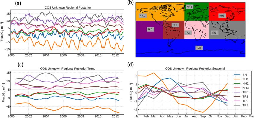
3514                                                                                  J. Ma et al.: Global inverse modelling of COS

Table 3. Names and error settings of the inversions performed in this study. The values correspond to grid-scale errors. Monthly flux fields
are optimized using spatial and temporal correlation lengths of 4000 km and 12 months, except for inversion Su , in which multiple settings
are explored.

                                      Biosphere   Ocean    Ocean     Biomass     Anthropogenic      Unknown
                                                  COS      CS2       burning     COS and CS2
                                 Su   –           –        –         –           –                  100 %
                                 S1   50 %        50 %     50 %      10 %        10 %               –
                                 S2   –           50 %     50 %      –           –                  –
                                 S3   50 %        –        –         –           –                  –

Note that this rate expression is independent of temperature            each cell) applied in the model as
and slightly different from that of Sander et al. (2006). This
latter rate was used in Khan et al. (2017) and resulted in a                   f gMair 1t
                                                                        σf =              .                                             (9)
short CS2 lifetime of 2.8–3.4 d. However, when we imple-                         MS 1p
ment the rate of Sander et al. (2006) in TM5, we find a CS2
                                                                        Here, f represents the sum of all COS prior flux compo-
lifetime of 6.2 d. This might be due to the fact that we ig-
                                                                        nents. In this sum, the biosphere flux is dominant over re-
nore CS2 deposition (15 % of the loss according to Khan
                                                                        gions with strong biosphere uptake. Further, g is gravita-
et al., 2017) or that we use lower OH or higher emissions.
                                                                        tional acceleration (9.8 m s−2 ), Mair is the molar mass of
Rate r2 = 2.0 × 10⁻¹² cm3 s−1 molecule−1 leads to an atmo-
                                                                        dry air (28.9 kg kmol−1 ), MS is the molar mass of sulfur
spheric CS2 lifetime of 9.4 d in TM5. Rate r3 represents an
                                                                        (32.1 kg kmol−1 ), 1p (Pa) is the thickness of the first model
exponential decay of 1.2 d for DMS (r3 = 9.6 × 10⁻⁶ s−1 ).
                                                                        layer and 1t is the time (s) over which the COS flux accu-
   COS photolysis frequencies are calculated based on a
                                                                        mulates (we use 1 h). Note that σf is unitless and is multiplied
troposphere ultraviolet and visible (TUV) radiation model
                                                                        by 1 × 10¹² to obtain units of pmol mol−1 .
(Madronich et al., 2003). Based on monthly climatologies
                                                                           Based on the total error, we define a χ 2 metric to quan-
of ozone profiles and temperatures, monthly averaged pho-
                                                                        tify how well the observations are reproduced by the model
tolysis frequencies are calculated on a 1 km grid span-
                                                                        (e.g. at a particular station).
ning 0–120 km and on 180 latitude bands. Implemented
in TM5, COS loss in the stratosphere amounts to about                          PN
                                                                                      (H x − y)2
40 Gg a−1 . This estimate is in line with earlier estimates of          χ 2 = i=1                  ,                                (10)
                                                                                      N σt2
(50 ± 15) Gg a−1 (Brühl et al., 2012; Barkley et al., 2008;
Chin and Davis, 1995; Engel and Schmidt, 1994; Weisen-                  where N is the number of individual observations. We can
stein, 1997; Krysztofiak et al., 2015; Turco et al., 1980;              calculate this metric before optimization (prior) and after op-
Crutzen and Schmailzl, 1983; Crutzen, 1976).                            timization (posterior). χ 2 is used to diagnose whether inver-
                                                                        sions are over-fitting or under-fitting the information con-
2.4    Model–data mismatch errors                                       tained in the measurement network. A value of χ 2 ≈ 1.0 in-
                                                                        dicates that the inverse system is able to fit the data within the
The diagonal elements of the error covariance matrix R in               error setting (Hooghiemstra et al., 2011). A large posterior
Eq. (5) contain contributions from observational errors, rep-           χ 2 indicates that the state does not have enough degrees of
resentation errors and errors related to applying large fluxes          freedom to fit the observations properly (or the error settings
in the planetary boundary layer (Bergamaschi et al., 2010):             are too small). A small posterior χ 2 indicates over-fitting of
       q                                                                the observations (or too wide error settings).
σt =       (σo2 + σr2 + σf2 ),                                 (8)      2.5    Model settings

where σt is the total error, σo the observational error, σr the         In this study, the TM5-4DVAR system is employed on a
representation error and σf an error related to applying large          global resolution of 6◦ ×4◦ (longitude × latitude). Flux fields
surface fluxes. The assumed observational error is shown in             are coarsened from a resolution of 1◦ × 1◦ . To create a
Fig. 3. It is worth noting that observational errors are usu-           reasonable start field for the inversions, we initially per-
ally overwhelmed by the representation and flux errors. The             formed an 11-year forward simulation starting with zero ini-
representation error is calculated by sampling the modelled             tial mole fractions and baseline surface fluxes augmented
gradients in the vicinity of the sampled station (Bergamaschi           by 432 Gg a−1 , distributed uniformly to close a gap in
et al., 2010). Finally, the flux error in each cell is linked to        the global budget. After 11 years, sources and sinks are
the magnitude of the monthly surface flux f (kg m−2 s−1 in              roughly in balance, with atmospheric mole fractions of about

Atmos. Chem. Phys., 21, 3507–3529, 2021                                                       https://doi.org/10.5194/acp-21-3507-2021
J. Ma et al.: Global inverse modelling of COS                                                                               3515

500 pmol mol−1 . Note that fluxes are used as zero-order           fluxes are less reliable, because they have not been well con-
terms, while the COS removal by OH and photolysis are              strained by observations. The optimized fluxes in the over-
first-order removal terms that grow as the atmospheric COS         lapping years are used to check the inversion results for con-
increases.                                                         sistency. In general, it is found that the optimized fluxes in
   We will present the results of four inversions. Firstly,        the overlapping periods are highly consistent.
we optimized the missing emissions, which amount to
432 Gg a−1 . This inversion will be denoted by Su through-
out the paper. The aim of this inversion is to investigate         3     Results
the spatial structure and temporal variability in the missing
COS emissions. This is the first time that a formal 4DVAR          3.1    Closing a gap in the COS budget
approach is applied to the COS budget. To this end, we
start from an emission field of 432 Gg a−1 that is uniformly       In this section, we consider inversion Su , in which a uniform
distributed globally. We optimize emissions on a monthly           field emitting 432 Gg a−1 is optimized. We use different set-
timescale and assign a grid-scale prior error of 100 %, which      tings for the spatial and temporal correlation lengths of this
is an arbitrary number to give fluxes enough freedom to ad-        field in the inversion and quantify the posterior goodness of
just. In a 3-year inversion, the total number of state vec-        fit using the χ 2 metric (Eq. 10). As presented in more de-
tor elements amounts to 97 200 (36 months × 45 latitudi-           tail in Fig. S5 we find, as expected, that χ 2 decreases with
nal bins × 60 longitudinal bins). The total number of NOAA         increasing degrees of freedom (smaller correlations).
observations is much smaller, thus rendering the inversion             Overall, the posterior fit to NOAA surface observations
under-determined. We therefore also use inversion Su to ex-        from 14 sites does not improve significantly for smaller cor-
plore different settings of the temporal and spatial correlation   relation lengths. If we analyse the posterior fit to the short-
lengths, which control the degrees of freedom of the state         term sampling programme from HIPPO, however, we find
vector. We explore spatial correlation lengths of 1000, 4000,      that the χ 2 reaches a minimum (see Fig. S5). After this min-
6000, 10 000 and 20 000 km and temporal correlation lengths        imum, χ 2 values increase again, a possible sign of over-
of 5.5, 7, 9.5 and 12 months.                                      fitting. We therefore select 4000 km and 12 months for the
   Secondly, we explore the optimization of specific cate-         spatial and temporal correlation length, respectively, and use
gories in inversions S1–S3. In S1 we attempt to perform an         these values in the remainder of this study.
“objective” inversion, in which we assign grid-scale errors of         Figure 4 presents the fit to observations of the prior and
50 % to the biosphere and ocean (we optimize both COS and          posterior simulation, for the inversion with temporal and spa-
CS2 ) and 10 % to the anthropogenic COS and CS2 emissions          tial correlation lengths of 12 months and 4000 km, respec-
and to the biomass burning emissions. Furthermore, in S2 we        tively. Corresponding χ 2 metrics per station are listed as la-
only optimize ocean exchange and in S3 we only optimize            bels in Fig. 4. Posterior fits are by design much better than
the biosphere exchange. The aim of inversions S1–S3 is to          prior fits. Only for NOAA stations THD and NWR does
explore whether either ocean fluxes or the biosphere fluxes        the posterior χ 2 remain larger than 3, indicating insufficient
(or both) should be used to close the gap in the COS bud-          degrees of freedom to resolve remaining discrepancies, un-
get. Note that DMS ocean emissions are not optimized. The          derestimated model errors or the influence of outliers (see
names and settings of the inversions are summarized in Ta-         Fig. 4g, h). THD is a coastal site (107 m a.s.l.), and NWR
ble 3.                                                             is a tundra site above the treeline (3526 m a.s.l.) in the USA
   The cost function is minimized with CONGRAD, an effi-           (Fig. 1), and thus the model resolution of 6◦ × 4◦ is likely
cient numerical algorithm for solving linear systems (Lanc-        too coarse to represent these sites. The local coastal effect
zos, 1950). This minimizer has also been used in previous in-      might be another reason why THD yields a larger χ 2 (Ri-
verse modelling studies with the TM5-4DVAR system (Basu            ley et al., 2005). It is worth noting that the posterior sim-
et al., 2013; Monteil et al., 2011, 2013; Houweling et al.,        ulation does not exhibit jumps in overlapping years from
2014; Pandey et al., 2015). For convergence, we request a          the parallel-running inversions, indicating that our inversion
gradient norm reduction of 1 × 10⁵ , and this reduction is usu-    strategy works well.
ally achieved within 40 iterations.                                    The correlation settings have a large impact on the op-
   We perform flux inversions for the period 2000–2012.            timized fluxes. Figure 5 shows the spatial distribution of
To decrease computational costs, we adopt the strategy to          the posterior flux field calculated with two different corre-
run parallel 3-year inversions, and we discard the optimized       lation settings. For correlations of 1000 km and 5.5 months
fluxes of the first 6 months (spin-up) and the last 6 months       (panel a) we detect a typical pattern that signals over-
(spin-down). For example, the first inversion targets the pe-      fitting of the observations. In such a pattern, the opti-
riod 1 January 2000 to 1 January 2003, the second inversion        mized flux displays hot spots close to measurement loca-
1 January 2002 to 1 January 2005 and so on. In the spin-           tions (e.g. THD, MLO, SMO). For very long spatial corre-
up period the fluxes in the first 6 months are used to ad-         lations, e.g. 20 000 km, posterior fits are poor (χ 2 > 6; see
just the imperfect initial condition. In the spin-down period,     Fig. S5) and optimized flux patterns show irregular behaviour

https://doi.org/10.5194/acp-21-3507-2021                                            Atmos. Chem. Phys., 21, 3507–3529, 2021
3516                                                                              J. Ma et al.: Global inverse modelling of COS

Figure 4. COS prior and posterior comparison at NOAA stations. Red dots and bars are NOAA measurements with errors. Blue and black
dots represent the posterior and prior simulation, respectively. Results are shown for inversion Su in which only the unknown emission
category is optimized.

(Fig. S6). Our best inversion (4000 km and 12 months)                derestimated emissions of COS or COS precursors in the
produces a smooth optimized flux without apparent spatial            prior), a signal from biomass burning or an overestimated
patterns near observational stations (Fig. 5b). This pattern         biosphere sink. The ocean-dominated region SH (blue) has
confirms the missing COS sources in the tropics (Sunthar-            a near-neutral flux, with a seasonal cycle that shows higher
alingam et al., 2008; Berry et al., 2013) and also requires          emissions in local autumn and early winter. In the next sec-
more uptake at high latitudes, especially in the NH.                 tion, we will explore the optimization of the ocean and bio-
   To investigate the variation in the optimized fluxes of in-       sphere fluxes.
version Su , we decompose the flux components as described
in Sect. 2.1.4. The monthly fluxes and derived long-term             3.2   Objective inversions
trend are shown in Fig. S7. The global flux was subsequently
split into eight regions, and the regional COS Su fluxes anal-       In this section we will discuss the results of inversions S1, S2
ysed for these regions are shown in Fig. 6. Region NH1               and S3. The resulting global budgets are compared to litera-
(North America plus part of the Pacific and Atlantic oceans,         ture values in Table 4. In addition, χ 2 metrics and biases of
orange) shows a negative “unknown” flux, indicating that             the various inversions are reported in Table 5 for the NOAA
more sinks are needed. This likely points to an underesti-           surface network, the HIPPO campaigns and the NOAA air-
mation of the biosphere uptake in the prior, since this region       borne profiles. Note that we also report results for optimiza-
(that is well constrained by observations) depicts a clear sea-      tions that assimilated the HIPPO observations besides the
sonal cycle in the optimized unknown flux.                           NOAA surface data. The period of the analysed inversions
   A larger sink is also needed in NH2 (Europe, green) and           is 2008–2010. The prior and posterior emission errors and
NH3 (Asia, red) but one of smaller magnitude than in NH1.            error reduction in the different inversion scenarios are listed
Tropical regions TR0–TR3 have a similar trend and season-            and discussed in Table S1.
ality and generally show a positive flux signal, with a small           The three inversions are all able to close the gap in the
seasonal cycle. This could represent an oceanic signal (un-          global COS budget with, however, very different budget

Atmos. Chem. Phys., 21, 3507–3529, 2021                                                https://doi.org/10.5194/acp-21-3507-2021
J. Ma et al.: Global inverse modelling of COS                                                                                                                 3517

Table 4. Results from inversions Su , S1, S2 and S3 compared to published global COS budgets. The total sources, total sinks, the unknown
flux and the total flux are shown in italics.

  COS budget (Gg a−1 )                      Kettle2002a        Montzka2007b            Berry2013c            Kuai2015d    Our prior      Su     S1      S2     S3
  Direct oceanic COS                                    41                     40                 39                41          40       40   −18       22     40
  Indirect oceanic CS2 as COS                           84                                        81                83          81       81     96     499     81
                                                                              240
  Indirect oceanic DMS as COS                          154                                       156               155         156      156    156     156    156
  Direct anthropogenic COS                              64                     64                 64                62         155      155    153     156    155
  Indirect anthropogenic                               116                       –               116               113         188      188    188     189    188
  CS2 as COS
  Indirect anthropogenic                                  1                      –                  1                0           6        6      6       6      6
  DMS as COS
  Biomass burning                                       38                    106                136                49         136      136    124     136    128
  Additional ocean flux                                   –                      –               600               559           –        –      –       –      –
  Anoxic soils                                          26                     66                   –                –           –        –      –       –      –
  Sources                                              523                    516              1193              1062          762      762    705    1163    754
  Destruction by OH                                   −94                    −96              −101               −111        −101     −101    −103   −101    −101
  Destruction by O                                    −11                    −11                    –                –           –        –      –       –      –
  Destruction by photolysis                           −16                    −16                    –                –        −40      −40    −40     −40    −40
  Uptake by plants                                  −238                  −1115               −738               −775
                                                                                                                            −1053     −1053   −557   −1053   −613
  Uptake by soil                                    −130                   −127               −355               −176
  Sinks                                              –489                  –1365              –1194             –1062       –1194     –1194   –700   –1194   –754
  Unknown                                                 –                      –                  –                –         432      425      –       –      –
  Net total                                             34                  –849                  –2                 0           0       –6      5     –31      0

a Kettle et al. (2002). b Table 2 from Montzka et al. (2007). c Berry et al. (2013). d Kuai et al. (2015).

terms (Table 4). Inversions S1 and S3 close the gap in the                                       problem: there are simply not enough observations in the
budget by a drastic reduction in the biosphere uptake in the                                     tropics to constrain the tropical fluxes. Fast mixing in the
tropics and more biosphere uptake at high latitudes. When                                        tropics further complicates the detection of signals from the
the biosphere is not optimized (S2), the inversion enhances                                      tropical biosphere using the NOAA surface network. With-
the CS2 tropical oceanic source and reduces direct COS                                           out additional observations it is therefore hard to unequiv-
emissions from the high-latitude oceans (Table 4). Both pat-                                     ocally close the gap in the tropical COS budget. Currently,
terns lead to reduced tropical biospheric uptake and more up-                                    inversion S1 mostly assigns the missing sources to reduced
take at high latitudes, as was found for inversion Su .                                          biosphere uptake in the tropics, but the superior Su inversion
   Concerning the posterior fit to observations, none of the                                     assigns the missing COS sources to a broad band in the trop-
S1–S3 inversions performed like inversion Su . The statistics                                    ics, without strong preference for land or ocean. Note that
in Table 5 show that Su leads to the best fit to the assimilated                                 the behaviour of inversions S1, S2 and S3 is strongly driven
observations and only a small remaining bias. Inversions S1                                      by the predefined spatio-temporal patterns in the prior flux
and S3 show better χ 2 statistics and smaller biases than in-                                    fields. In Sect. 3.4, we will revisit this issue.
version S2, because it is difficult to fit continental NOAA                                         Although we currently cannot close the gap in the global
stations (LEF, HFM, NWR, THD) only by optimizing ocean                                           COS budget with one specific known flux, it is instructive
fluxes. However, S1 and S3 show a tendency to turn the trop-                                     to explore the information content of a separate set of COS
ical biosphere sink into a source, as shown in Fig. 7, which                                     observations. In the next section, we will therefore evaluate
depicts the posterior biosphere flux and flux increment for                                      the results of our inversions with HIPPO and NOAA airborne
inversion S1. Note that while the uptake over high NH lati-                                      observations (Fig. 1).
tudes is enhanced, fluxes over regions in South America and
over Indonesia have turned into a source. This behaviour can
be explained by the under-determined nature of the inverse

https://doi.org/10.5194/acp-21-3507-2021                                                                                 Atmos. Chem. Phys., 21, 3507–3529, 2021
3518 J. Ma et al.: Global inverse modelling of COS
vations from the NOAA airborne profiles, which are mostly
collected over the USA (see Fig. 1). Figure 9 shows a com-
parison between profiles using results of inversion S1. Al-
though most posterior profiles (blue) improve considerably
compared to the prior simulation (black), they still underesti-
mate observations (red) in the free troposphere. Note that the
simulations based on inversion S1 correctly predict the draw-
down of COS towards the surface for most measured profiles,
and in particular the match with the LEF site is very good at
the surface, which confirms the performance of the inversion.
If HIPPO observations are additionally assimilated (green),
the agreement in the free troposphere slightly improves. For
S1, χ 2 for the profile comparison reduces from 27.7 to 20.1
and the bias reduces from −13.9 to −9.7 pmol mol−1 (Ta-
ble 5). This confirms the low bias of the free troposphere
COS mole fractions in simulations with fluxes that are opti-
mized using both NOAA surface and HIPPO observations.
It is now clear that inversions using surface data from the
available NOAA network sites will not be able to separate
various source categories and specifically not in the data-void
Figure 5. Optimized emission pattern of the unknown field of in-
version Su for different settings of the spatio-temporal correlation tropics. In the next section we will therefore investigate the
lengths. (a) Spatial correlation of 1000 km and temporal correlation prospects of using satellite data to constrain fluxes.
of 5.5 months. (b) Spatial correlation of 4000 km and temporal cor-
relation of 12 months. Results are averages over 2008–2011. 3.4 Satellite validation
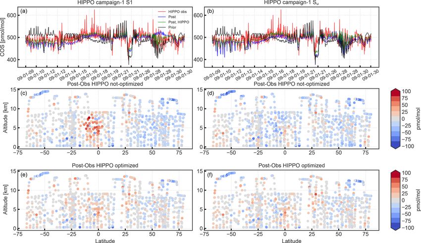
In Fig. 10 we present a comparison between MIPAS, ACE-
3.3 Evaluation with HIPPO and NOAA airborne FTS and co-sampled TM5 COS profiles. The latitude–height
profiles distributions of MIPAS, TM5 (convolved with the MIPAS
AK) and ACE-FTS are shown in Fig. 10a–c. In Fig. 10d
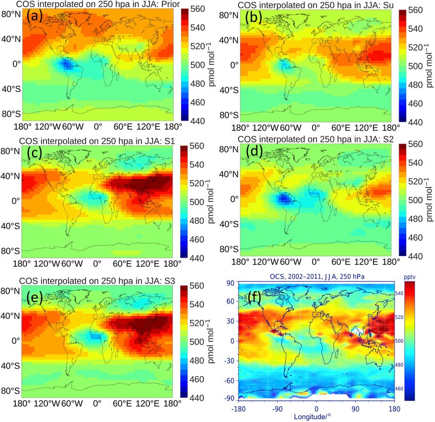
From Table 5 it is clear that for all inversions the comparison we show averaged ACE-FTS, MIPAS and TM5 profiles, the
to HIPPO observations is not very favourable. Most notably, latter two resulting from collocations with respect to ACE-
the simulations with optimized fluxes show strong negative FTS. The TM5 profiles shown are from the prior simulation
biases and poor χ 2 statistics. However, Fig. 8 shows that the (black), from inversion S1 (blue) and from inversion S1 with
inversions S1 and Su (blue lines) largely improve the cor- additional assimilation of HIPPO profiles (green). They are
respondence to HIPPO campaign-1 observations (red), rela- all convolved with the MIPAS AK.
tive to the prior simulation (black). The posterior simulations In general, TM5 reproduces the observed pattern of COS
capture the HIPPO observations much better. The remaining well but with lower values in the tropical upwelling region
differences in the middle panels of Fig. 8 show the general at around a 25 km altitude. The comparison between ACE-
underestimation of the model. However, inversion S1 over- FTS and MIPAS is consistent with findings of Glatthor et al.
estimates HIPPO in the southern tropics, likely caused by (2017), who found that ACE-FTS is systematically lower in
too large flux adjustments over South America, the region the UTLS region. Moreover, they found that MIPAS data
sampled by HIPPO campaign 1. showed no bias compared to MkIV and SPIRALE COS bal-
Interestingly, when the HIPPO observations are addition- loon profiles, which also exhibit higher COS values than
ally assimilated into the inversion, biases are largely removed ACE-FTS (Krysztofiak et al., 2015; Velazco et al., 2011).
(Fig. 8, lower panels) while the correspondence to the NOAA TM5 profiles, after convolution with the MIPAS AK, are
surface network deteriorates only slightly (Table 5). Posterior in between MIPAS and ACE-FTS. Compared to the other
χ 2 values for the HIPPO campaigns remain relatively poor, TM5 runs, prior TM5 profiles (black) show the lowest val-
however, signalling too strict error settings or processes that ues around the tropopause. Again, TM5 profiles optimized
are not properly modelled. by HIPPO and NOAA observations (dashed green line in
From the comparison with HIPPO we find that our state Fig. 10d) show a slight increase in the upper troposphere
vector has enough flexibility to fit additional observations compared to the optimization with only NOAA surface-site
and that the inversions are strongly observation-limited. data (dashed blue line).
Moreover, we find that the inversions based on only observa- To compare the different inversions with respect to the
tions from the NOAA surface network tend to underestimate simulated latitude–longitude distribution, Fig. 11 shows a
COS in the free troposphere. This is corroborated by obser- comparison of COS between TM5 inversions and MIPAS at
Atmos. Chem. Phys., 21, 3507–3529, 2021 https://doi.org/10.5194/acp-21-3507-2021J. Ma et al.: Global inverse modelling of COS 3519
Figure 6. Regional analysis of multi-year optimized COS fluxes of inversion Su : (a) posterior flux per region, (b) regions over which the
posterior flux is analysed, (c) trend in the decomposed signal and (d) seasonal signal in the decomposed signal. Note that region colours in
(b) are used in (a), (c) and (d).
Table 5. χ 2 metrics and mean biases for the different inversion
scenarios. Statistics are shown for the NOAA surface stations, the
HIPPO campaigns and the NOAA airborne profiles. Biases are
given in pmol mol−1 .
Inversion HIPPO Metric HIPPO NOAA NOAA
scenario optimized∗ surface airborne
No χ2 40.7 1.9 26.0
No Bias −13.9 0.0 −12.4
Su
Yes χ2 4.7 2.5 17.3
Yes Bias −1.1 1.5 −8.3
No χ2 43.8 2.4 27.7
No Bias −12.0 −0.4 −13.8
S1
Yes χ2 4.8 2.9 20.1
Yes Bias −1.3 1.3 −9.7
No χ2 54.2 4.9 48.2
No Bias −19.4 1.5 −16.7
S2
Yes χ2 6.3 5.9 27.0
Yes Bias −4.6 7.5 −5.9
No χ2 43.3 2.5 27.5
No Bias −12.3 −0.2 −14.3 Figure 7. Posterior biosphere flux from inversion S1 and increment
S3
Yes χ2 5.0 3.2 21.1 (posterior–prior). The fluxes represent 3-year (2008–2010) averages
Yes Bias −1.4 1.6 −10.5 with removal of 6-month spin-up and spin-down periods. The max-
∗ If HIPPO is not optimized, only NOAA surface data are assimilated into inversions. If imum and minimum flux values are given in the boxes.
HIPPO is optimized, both NOAA surface data and HIPPO are assimilated into inversions.
NOAA airborne data are only used for validation.
https://doi.org/10.5194/acp-21-3507-2021 Atmos. Chem. Phys., 21, 3507–3529, 20213520 J. Ma et al.: Global inverse modelling of COS
Figure 8. HIPPO campaign-1 COS observations compared to results from inversions S1 (a, c, e) and Su (b, d, f). The first row shows
time series of HIPPO observations (red), prior (black), posterior (blue), and posterior with HIPPO observations assimilated (green). The
middle and bottom rows show the model minus observations in a latitude–height plot for inversions with and without assimilating HIPPO
observations, respectively.
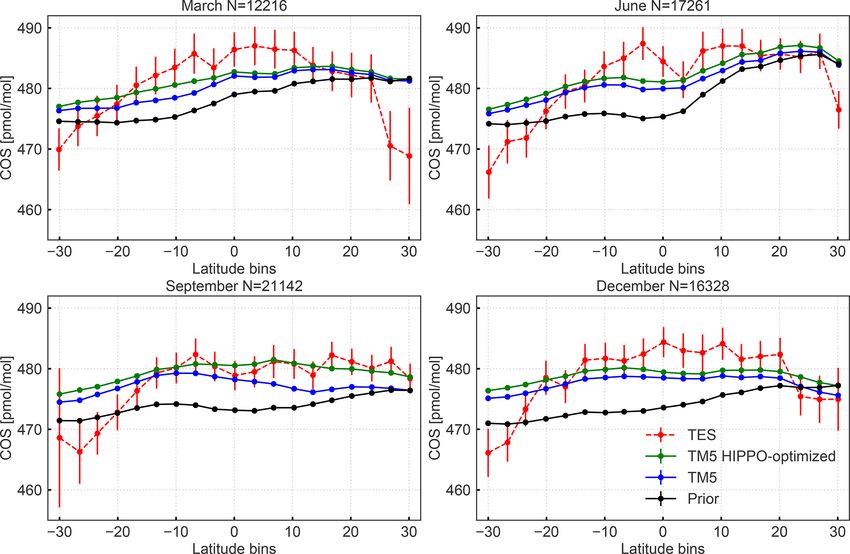
250 hPa in June to August. Similar results at 250 hPa from itudinal bins between 32◦ S and 32◦ N. Outside this latitude
September to November and at 150 hPa from June to Au- band, TES observations become too noisy for a reasonable
gust are shown in the Supplement (Figs. S8 and S9). MIPAS comparison. Comparisons are shown for the months March,
COS represents a 2002–2011 average taken from Glatthor June, September and December in Fig. 12, based on inver-
et al. (2017). TM5 results have been averaged over 2008– sion S1 and averaged over the years 2008–2011. We applied
2010. The distributions of COS in all inversions match rela- an arbitrary bias correction of β = 1 in Eq. (1) to obtain a
tively well with MIPAS. Note, however, that we adjusted the reasonable fit to TES observations. After assimilation, the
TM5 results by +25 pmol mol−1 to match the colour scale agreement with TES improves compared to the prior, but the
of MIPAS. The COS distribution from the prior simulation latitudinal gradients remain generally smaller in the model.
correctly simulates low COS over the Amazon and Africa The inversion into which the HIPPO observations are also as-
but is clearly too high over northern latitudes. This latter as- similated increases the simulated mole fractions, confirming
pect is partly solved by the inversions. If we concentrate on our findings based on the airborne observation. In general,
the observed COS minimum over the Atlantic, Africa and the the TES-derived columns offer a good perspective to better
Amazon, inversions S1 and S3 shift this minimum to the east, constrain the COS budget in the tropics. Due to the sensitivity
consistent with the COS biosphere flux increment shown in of TES to COS in the middle troposphere (Kuai et al., 2015),
Fig. 7 for S1. Inversions Su and S2 exhibit a better compari- the assimilation of TES into our 4DVAR system might be
son with MIPAS, suggesting that the large increments of the able to differentiate between the biosphere and ocean signal,
tropical biosphere over South America (Fig. 7) are unrealis- something that turned out to be difficult using NOAA surface
tic. However, assigning the missing tropical source totally to observations only.
ocean emissions (S2) appears to overestimate the COS draw-
down over the Amazon. 3.5 Discussion
TM5 results are also compared to the nadir-viewing TES
instrument. To this end, COS columns of TM5 (convolved
In this study we have presented inversions focused on the
with the TES AK; see Eq. 1) and TES are averaged in 20 lat-
closure of the global COS budget. In general, our inversion
Atmos. Chem. Phys., 21, 3507–3529, 2021 https://doi.org/10.5194/acp-21-3507-2021You can also read