Implementation of sequential cropping into JULESvn5.2 land-surface model
←
→
Page content transcription
If your browser does not render page correctly, please read the page content below
Geosci. Model Dev., 14, 437–471, 2021
https://doi.org/10.5194/gmd-14-437-2021
© Author(s) 2021. This work is distributed under
the Creative Commons Attribution 4.0 License.

Implementation of sequential cropping into
JULESvn5.2 land-surface model
Camilla Mathison1,2 , Andrew J. Challinor2 , Chetan Deva2 , Pete Falloon1 , Sébastien Garrigues3,4 , Sophie Moulin4 ,
Karina Williams1,5 , and Andy Wiltshire1,5
1 Met Office Hadley Centre, FitzRoy Road, Exeter, UK
2 School of Earth and Environment, Institute for Climate and Atmospheric Science, University of Leeds, Leeds, UK
3 European Centre for Medium-Range Weather Forecasts, Reading, UK
4 Environnement Méditerranéen et Modélisation des AgroHydrosystèmes (EMMAH), INRAE, Avignon Université,

228 route de l’Aérodrome Domaine Saint Paul–Site Agroparc, Avignon, France
5 Global Systems Institute, University of Exeter, Laver Building, North Park Road, Exeter, UK

Correspondence: Camilla Mathison (camilla.mathison@metoffice.gov.uk)

Received: 29 March 2019 – Discussion started: 25 April 2019
Revised: 6 October 2020 – Accepted: 4 December 2020 – Published: 25 January 2021

Abstract. Land-surface models (LSMs) typically simulate a        quential cropping method affects the available soil moisture
single crop per year in a field or location. However, actual     in the top 1.0 m throughout the year, with larger fluctuations
cropping systems are characterized by a succession of dis-       in sequential crops compared with single-crop simulations
tinct crop cycles that are sometimes interspersed with long      even outside the secondary crop growing period. JULES sim-
periods of bare soil. Sequential cropping (also known as mul-    ulates sequential cropping in Avignon, the four India loca-
tiple or double cropping) is particularly common in tropi-       tions and the regional run, representing both crops within one
cal regions, where the crop seasons are largely dictated by      growing season in each of the crop rotations presented. This
the main wet season. In this paper, we implement sequen-         development is a step forward in the ability of JULES to sim-
tial cropping in a branch of the Joint UK Land Environment       ulate crops in tropical regions where this cropping system is
Simulator (JULES) and demonstrate its use at sites in France     already prevalent. It also provides the opportunity to assess
and India. We simulate all the crops grown within a year         the potential for other regions to implement sequential crop-
in a field or location in a seamless way to understand how       ping as an adaptation to climate change.
sequential cropping influences the surface fluxes of a land-
surface model. We evaluate JULES with sequential cropping
in Avignon, France, providing over 15 years of continuous
flux observations (a point simulation). We apply JULES with      1   Introduction
sequential cropping to simulate the rice–wheat rotation in a
regional 25 km resolution gridded simulation for the northern    Climate change is likely to impact all aspects of crop pro-
Indian states of Uttar Pradesh and Bihar and four single-grid-   duction, affecting plant growth, development and crop yield
box simulations across these states, where each simulation       (Hatfield and Prueger, 2015) as well as cropping area and
is a 25 km grid box. The inclusion of a secondary crop in        cropping intensity (Iizumi and Ramankutty, 2015). The im-
JULES using the sequential cropping method presented does        pact of climate change on agriculture has been the focus of
not change the crop growth or development of the primary         several large collaborative projects such as the Agricultural
crop. During the secondary crop growing period, the carbon       Model Intercomparison and Improvement Project (AgMIP;
and energy fluxes for Avignon and India are modified; they       Rivington and Koo, 2010; Rosenzweig et al., 2013, 2014)
are largely unchanged for the primary crop growing period.       and the Inter-Sectoral Impact Model Intercomparison Project
For India, the inclusion of a secondary crop using this se-      (ISIMIP; Warszawski et al., 2013, 2014). These projects
                                                                 have highlighted the likelihood of competition between crops

Published by Copernicus Publications on behalf of the European Geosciences Union.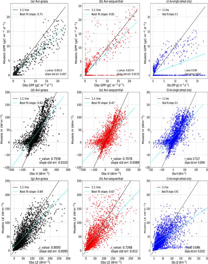
438                       C. Mathison et al.: Implementation of sequential cropping into JULESv5.2 land-surface model

grown for food and those grown for bio-energy in order to         1.1   Modelling sequential cropping in land-surface
mitigate climate change (Frieler et al., 2015). Petrie et al.           models
(2017) discuss how the use of sequential cropping systems
may have made it possible for populations in some areas to        The modelling of crop rotations is a regular feature of
adapt to large changes in monsoon rainfall between 2200 and       soil carbon simulations (Bhattacharyya et al., 2007). Bhat-
2100 BC. These ancient agricultural practices are common          tacharyya et al. (2007) found that the rice–wheat rotation,
today across most tropical countries but may also be a useful     common across the IGP, has helped maintain carbon stocks.
adaptation in areas where traditionally mono-crop systems         However, in recent years, the yields of rice and wheat have
are used, in order to meet a future rising demand for food        plateaued, leading farmers to diversify and include other ad-
(Hudson, 2009) or the demand for bio-fuels. This sort of          ditional crops in the rotation, potentially depleting carbon
adaptation is already happening in some locations. Mueller        stocks. The modelling of crop rotations has also been rep-
et al. (2015) show that longer growing seasons in the extrat-     resented in the field of agricultural economics with work
ropics have made the cultivation of multiple crops in a year at   regarding sequential cropping being mainly to understand
northern latitudes more viable. Warmer spring temperatures        influences on decision-making, therefore focusing on short
in the Brahmaputra catchment have allowed earlier planting        timescales and at the farm management level (Dury et al.,
of a winter crop, leaving time for a second crop (Zhang et al.,   2012; Caldwell and Hansen, 1993).
2013).                                                               Many dynamic global vegetation models (DGVMs), used
   The economy of South Asia is highly dependent on the           to study the effects of climate change, simulate a single crop
agricultural industry and other industries also with a high de-   in a field per year, both for individual sites and gridded sim-
mand for water (Mathison et al., 2015). The most important        ulations. This may be due in part to some global observation
source of water for this part of the world is the Asian summer    datasets such as Sacks et al. (2010) reporting only one grow-
monsoon (ASM), which typically occurs between June and            ing period per year at a given location for most crops (Waha
September (Goswami and Xavier, 2005); this phenomenon             et al., 2012). Where different crop calendars are available for
provides most of the water resource for any given year. The       different regions, e.g. MIRCA2000 (Portmann et al., 2010),
South Asian crop calendar is defined by the ASM, which has        rice and wheat are divided equally between the kharif (i.e.
an important influence on the productivity across the whole       sown during the monsoon and harvested during the autumn)
year (Mathison et al., 2018), thereby affecting crop produc-      and rabi seasons (i.e. the drier winter/spring growing season),
tion outside the monsoon period.                                  when in reality wheat is only grown during the rabi season
   Intercropping or sequential cropping allow farmers to          (Biemans et al., 2016).
make the most efficient use of limited resources and space in        The Lund–Potsdam–Jena managed land model (LPJml;
order to maximize yield potential and lower the risk of com-      Bondeau et al., 2007; Schaphoff et al., 2018) is one of the
plete crop failure. These techniques also influence ground        few models that is able to simulate sequential cropping. Waha
cover, soil erosion and chemical properties, albedo and pest      et al. (2013) extend LPJml to consider sequential cropping in
infestation (Waha et al., 2013). Intercropping is the simul-      Africa for two different crops on the same field within a year.
taneous cultivation of multiple crop species in a single field    Waha et al. (2013) specify different growing periods for each
(Cong et al., 2015), while sequential cropping (also called       crop in the rotation, where the growing period is calculated
multiple or double cropping) involves growing two or more         from the sum of the daily temperatures above a crop-specific
crops on the same field in a given year (Liu et al., 2013;        temperature threshold. Waha et al. (2013) use the Waha et al.
Waha et al., 2013). We use the term sequential cropping from      (2012) method to specify the onset of the main rainy season
here on to avoid confusion with other cropping systems. Se-       as the start of the growing season, where growing season is
quential cropping systems are common in Brazil where the          defined as the period of time in which temperature and mois-
soybean–maize or soybean–cotton rotations are used (Pires         ture conditions are suitable for crop growth. The growing pe-
et al., 2016) and for South Asia where the rice–wheat systems     riod of the first crop in the rotation begins on the first wet day
are the most extensive, dominating in many Indian states          of the growing season, with the second crop assumed to start
(Mahajan and Gupta, 2009), across the Indo-Gangetic Plain         immediately after harvest of the first crop. Waha et al. (2013)
(IGP) (Erenstein and Laxmi, 2008) and Pakistan (Erenstein         find that when considering the impact of climate change, the
et al., 2008). States such as Punjab, Haryana, Bihar, Uttar       type of cropping system is important because yields differ
Pradesh and Madhya Pradesh (Mahajan and Gupta, 2009) ac-          between crops and cropping systems. Biemans et al. (2016)
count for approximately 75 % of national food grain produc-       also use a version of LPJml refined for South Asia to estimate
tion for India. Rice–rice rotations are the second most preva-    water demand and crop production for South Asia. Biemans
lent crop rotation to rice–wheat rotations; these are typically   et al. (2016) combine the output from two separate simula-
found in the northeastern regions of India and Bangladesh         tions, each with different kharif and rabi land-use maps and
(Sharma and Sharma, 2015), with some regions cultivating          zonal sowing and harvest dates based on observed monsoon
as many as three rice crops per year.                             patterns. Biemans et al. (2016) find that accounting for multi-
                                                                  ple different crops being grown on the same area at different

Geosci. Model Dev., 14, 437–471, 2021                                               https://doi.org/10.5194/gmd-14-437-2021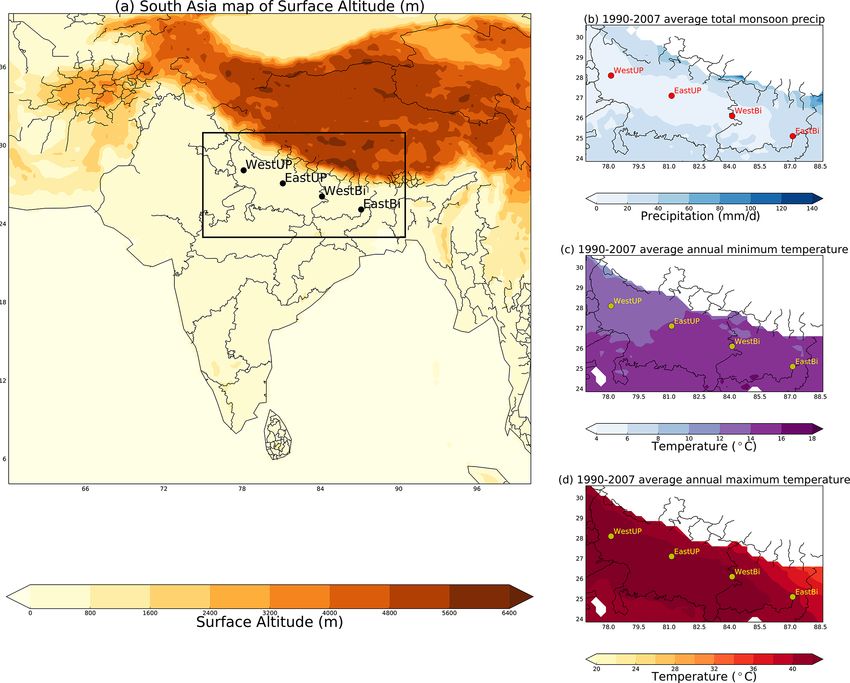
C. Mathison et al.: Implementation of sequential cropping into JULESv5.2 land-surface model                                     439

times of the year improves the simulations of demand for           sequential cropping are provided in Sect. 5 and discussed in
water for irrigation, particularly the timing of the demand.       Sect. 6, with conclusions in Sect. 7.
Waha et al. (2013) and Biemans et al. (2016) simulate more
than one crop growing on the same area using very different
methods; both have highlighted the importance of represent-        2     The JULES-crop model
ing this type of cropping system.
   Garrigues et al. (2015a) demonstrate that the Interactions      2.1    Model description
between the Soil, Biosphere and Atmosphere (ISBA) land-
surface model (LSM) (Noilhan and Planton, 1989), specifi-          The JULES model is the land-surface scheme used by the
cally ISBA-A-gs (Calvet et al., 1998), is able to represent a      UK Met Office for both weather and climate applications. It
12-year succession of arable Mediterranean crops for a site        is also a community model and can be used in stand-alone
in Avignon, France (Garrigues et al., 2015a, b). This type of      mode, which is how it is used in the work presented here.
cropping system is not typically represented in LSMs; how-         The parameterization of crops in JULES (JULES-crop) is de-
ever, this study showed that the implementation of crop suc-       scribed in Osborne et al. (2015) and Williams et al. (2017).
cessions in an LSM leads to a more accurate representation         JULES-crop is a dual-purpose crop model intended for use
of cumulative evapotranspiration over the 12-year period. It       within stand-alone JULES, enabling a focus on food pro-
would be beneficial for more land-surface models to develop        duction and water availability applications, and as the land-
the capability to simulate different cropping systems and link     surface scheme within climate and Earth system models.
crop production with irrigation both to improve the represen-      JULES-crop has been used in stand-alone mode in recent
tation of the land surface in coupled models and to improve        studies such as Williams and Falloon (2015) and Williams
climate impacts assessments.                                       et al. (2017). The aim is that these studies and this one will
   In this paper, we describe and implement sequential crop-       lead to using JULES in these larger models to allow the feed-
ping in the Joint UK Land Environment Simulator (JULES).           backs from regions with extensive croplands and irrigation
We simulate the same Avignon site described in Garrigues           systems, like South Asia, to have an effect on the atmosphere,
et al. (2015a, 2018) and two states in India to illustrate and     e.g. via methane emissions from rice paddies or evaporation
evaluate the method implemented in the JULES stand-alone           from irrigated fields (Betts, 2005).
model at version 5.2 for simulating sequential-crop rotations.        JULES is a process-based model that simulates the fluxes
By using Avignon and India, we simulate two types of crop          of carbon, water, energy and momentum between the land
rotation. We define the Avignon crop rotation as an irregu-        surface and the atmosphere. JULES represents both veg-
lar crop rotation due to the occurrence of long fallow peri-       etation (including natural vegetation and crops) and non-
ods, with extended periods of bare or almost bare soil. There      vegetation surface types including; urban areas, bare soil,
are no long fallow periods in the rice–wheat rotation for the      lakes and ice. With the exception of the ice tile, all these tiles
northern Indian states of Uttar Pradesh and Bihar, so we refer     can co-exist within a grid box so that a fraction of the surface
to this as a regular crop rotation. The rice–wheat rotation is     within each grid box is allocated between surface types. For
the dominant cropping system for Uttar Pradesh and Bihar,          the ice tile, a grid box must be either completely covered in
with these states being key producers of these crops. Sequen-      ice or not (Shannon et al., 2019). JULES treats each vegeta-
tial cropping is used in a series of single-grid-box simulations   tion type as a separate tile within a grid box, with each one
(where each grid box is 25 km) across these two states for         represented individually with its own set of parameters and
comparison with a point simulation in Avignon. We also use         properties, such that each tile has a separate energy balance.
sequential cropping in a regional 25 km resolution gridded         The model and the equations it is based on are described in
simulation to demonstrate that this method can be applied at       detail in Best et al. (2011) and Clark et al. (2011). Prognostics
larger scales. In the India simulations (both the regional and     such as leaf area index (LAI) and canopy height are therefore
single grid box), the model uses standard soil parameters,         available for each tile. The forcing air temperature, humidity
with meteorological information provided from a regional           and wind speed are prescribed for the grid box as a whole for
climate simulation (Sect. 3.2). However, for the point sim-        a given height. Below the surface, the soil type is also uni-
ulation in Avignon, we use the site characteristics and me-        form across each grid box (where the number of soil tiles is
teorological information from the site itself (Sect. 3.1). This    set to 1). We use JULES-crop (Osborne et al., 2015; Williams
paper is structured as follows: Sect. 2 describes the JULES-       et al., 2017) to simulate the crops in this study. The main
crop model, the rationale and the method for implementing          aim of JULES-crop is to improve the simulation of land–
sequential cropping in JULES. The simulations are described        atmosphere interactions where crops are a major feature of
in Sect. 3. In Sect. 4, we present our hypotheses for assessing    the land surface (Osborne et al., 2015).
the impact of sequential cropping in JULES, discuss the cli-          Photosynthesis in JULES-crop uses the same parameters
mate of the simulated regions and describe the observations        and code as the natural plant functional types (PFTs). There
we use to evaluate the model. The results from the evalua-         are two temperature parameters: Tlow and Tupp ; these define
tion of the simulations and the assessment of the impact of        the upper and lower temperature parameters for leaf bio-

https://doi.org/10.5194/gmd-14-437-2021                                                 Geosci. Model Dev., 14, 437–471, 2021

440                               C. Mathison et al.: Implementation of sequential cropping into JULESv5.2 land-surface model

Table 1. JULES flags used that are new or different from those in Osborne et al. (2015).

      Flag                           JULES                     Avignon         India           Effect
                                     notation                  settings        settings        of switch
      Canopy radiation               can_rad_mod               6               6               Selects the canopy radiation scheme.
      scheme
      Irrigation demand              l_irrig_dmd               F               T               Switches on irrigation demand.
      Irrigation scheme              irr_crop                  –               2               Irrigation occurs when the DVI of the
                                                                                               crop is greater than 0.
      Physiology                     l_trait_phys              F               F               Switches on trait-based physiology
                                                                                               when true.
      Sowing                         l_prescsow                T               T               Selects prescribed sowing.
      Plant maintenance              l_scale_resp_pm           F               F               Switch to scale respiration by water
      respiration                                                                              stress factor. If false, this is leaf respira-
                                                                                               tion only, but if true, it includes all plant
                                                                                               maintenance respiration.
      Crop rotation                  l_croprotate              T               T               A new switch to use the sequential crop-
                                                                                               ping capability.
      Irrigation on tiles            frac_irrig_all_tiles      –               F               Switch to allow irrigation on all or spe-
                                                                                               cific tiles.
      Irrigation on specific         set_irrfrac_on_irrtiles   –               T               A new switch to set irrigation to only
      tiles                                                                                    occur on a specific tile.
      Specify irrigated tile(s)      irrigtiles                –               6               Setting to set the value(s) of the specific
                                                                                               tile(s) to be irrigated.
      Number of tiles                nirrtile                  –               1               Setting to set how many tile(s) are to be
      irrigated                                                                                irrigated.
      Set a constant irrigation      const_irrfrac_irrtiles    –               1.0             A new setting to set the value(s) of the
      fraction                                                                                 irrigation fraction for specific tile(s) to
                                                                                               be irrigated in the absence of a file of
                                                                                               irrigation fractions.

chemistry and photosynthesis within JULES (Clark et al.,                  ductivity (NPP) is GPP minus plant respiration; NPP is used
2011) and are used to calculate the maximum rate of car-                  in the crop partitioning code and subsequently in the calcu-
boxylation of RuBisCO (unstressed by water availability and               lation of the yield in JULES. The nitrogen cycle in JULES
ozone effects – Vcmax , with units of mol CO2 m−2 s−1 ), as               cannot yet be used with the crop model, so in this study the
defined in Clark et al. (2011) and reproduced here in Eq. (1).            same assumption is made as in Williams et al. (2017): that
Equation (1) demonstrates the Vcmax at any desired tempera-               crops are not nitrogen limited.
ture.                                                                        The effective temperature (Eq. 3) is the function that the
                       neff nl (0) fT (Tc )                               model uses to relate air or leaf temperature to the cardinal
Vcmax =                                                           (1)    temperatures that define a plant’s development; these are the
             1 + e0.3(Tc −Tupp ) 1 + e0.3(Tlow −Tc )

                                                                          base temperature (Tb ), maximum temperature (Tm ) and op-
               0.1(T −25)
fT (Tc ) = Q10leafc         ,                                      (2)    timum temperature (To ) and are specific for each crop. Dif-
                                                                          ferent models define their effective temperature function in
where fT is the standard Q10 temperature dependence (given
                                                                          different ways; for example, Fig. 1 of Wang et al. (2017) pro-
in Eq. 2) and Tc is the canopy temperature. neff repre-
                                                                          vides a number of different possible definitions. The JULES
sents the scale factor in the Vcmax calculation (in units of
                                                                          definition described by Eq. (3) is most similar to type 4 given
mol CO2 m−2 s−1 kg C(kg N)−1 ) and nl (0) the top leaf nitro-
                                                                          in Wang et al. (2017). Type 4 increases gradually towards the
gen concentration (in units of kg N (kg C)−1 ). More details
                                                                          optimum temperature with a steeper decline from the opti-
regarding the calculation of Vcmax are provided in Clark et al.
                                                                          mum to the maximum. Other functions have no decline or a
(2011) and Williams et al. (2017). Vcmax is an important
                                                                          flatter top, which can have different effects on the develop-
component in two limiting factors for photosynthesis: the
                                                                          ment of the crop. In JULES, the cardinal temperatures and
RuBisCO-limited rate and the rate of transport of photosyn-
                                                                          the 1.5 m tile (i.e. air) temperature (T ) are used to calculate
thetic products; Eq. (1) shows the relationship between Vcmax
                                                                          the thermal time, i.e. the accumulated effective temperature
and temperature. Gross primary productivity (GPP) is used
                                                                          (Teff ) to which a crop is exposed (Osborne et al., 2015). Ta-
to describe the total productivity of a plant; this defines the
                                                                          ble 3 summarizes the settings for these temperatures used in
gross carbon assimilation in a given time. Net primary pro-

Geosci. Model Dev., 14, 437–471, 2021                                                       https://doi.org/10.5194/gmd-14-437-2021
C. Mathison et al.: Implementation of sequential cropping into JULESv5.2 land-surface model 441
Table 2. JULES plant functional type (PFT) parameters and values modified for use in this study. We include only the values that have been
changed or are new in JULES since Osborne et al. (2015).
Parameter JULES nota- Description (units) Winter wheat Sorghum Spring wheat Rice
tion
Tlow t_low_io Lower temperature for photosynthesis 5 18 5 15
(◦ C).
Tupp t_upp_io Upper temperature for photosynthesis 30 53 30 40
(◦ C).
neff neff_io Scale factor relating Vcmax with leaf ni- 0.8e-3 0.75e-3 0.8e-3 0.95e-3
trogen concentration.
nl (0) nl0_io Top leaf nitrogen concentration 0.073 0.07 0.073 0.073
(kg N (kg C)−1 .
fsmc method fsmc_mod_io When equal to 0, we assume an expo- 0 0
nential root distribution with depth.
When equal to 1, the soil moisture 1 1
availability factor, fsmc, is calculated
using average properties for the root
zone.
dr rootd_ft_io If fsmc_mod_io = 0, dr is the e-folding 0.5 0.5
depth (m).
If fsmc_mod_io = 1, dr is the total depth 1.5 1.5
of the root zone (m).
p0 fsmc_p0_io Parameter governing the threshold at 0.5 0.5 0.5 0.5
which the plant starts to experience wa-
ter stress due to lack of water in the soil.
µrl nr_nl_io Ratio of root nitrogen concentration to 0.39 0.39 0.39 0.39
leaf nitrogen concentration.
µsl ns_nl_io Ratio of stem nitrogen concentration to 0.43 0.43 0.43 0.43
leaf nitrogen concentration.
Q10,leaf q10_leaf_io Q10 factor in the Vcmax calculation. 1.0 1.0 1.0 1.0
this analysis. The crop model integrates an effective temper- crease of the development index, described by Eq. (4):
ature over time as the crop develops through these stages, T
eff
with the carbon partitioned according to the development in-
TTemr for −1 ≤ DVI < 0
dex (DVI). dDVI Teff
= TTveg for 0 ≤ DVI < 1 (4)
0 for T < Tb dt
Teff
for 1 ≤ DVI < 2,
T − Tb for Tb ≤ T ≤ To
TTrep
T − To
Teff = (To − Tb ) 1 − for To < T < Tm (3)
T m − T o where TTemr is the thermal time between sowing and emer-
0 for T ≥ Tm
gence, TTveg and TTrep are the thermal time between emer-
The DVI is a function of the thermal time since emergence; gence and flowering and between flowering and maturity, re-
therefore, DVI of −1 is sowing, 0 is emergence, and 1 is spectively. These are calculated either using a temperature
flowering. Maturity and therefore harvest occur at a DVI of climatology from the driving data and sowing dates from ob-
2 (Osborne et al., 2015) under standard growth conditions servations or using the method presented in Mathison et al.
but may be harvested earlier in other situations in the model (2018) to create a reliable sowing and harvest dataset. The
(Williams et al., 2017). In reality, the maturity date and the advantage of using the Mathison et al. (2018) method is that
harvest dates are not usually the same date. The integrated there are no missing data, which is often the case when using
effective temperature in each development stage is referred observed data. Whichever source of sowing and harvest dates
to as the thermal time of that development stage (Eq. 3 and are used, the aim is for the crop to reach maturity, on average
Osborne et al., 2015; Mathison et al., 2018). by the harvest date. The sowing and harvest dates used in the
Crop development can also be affected by the length of simulations in this analysis are described in Sect. 3.
the day. However, in these simulations, as in Osborne et al.
(2015), this effect is not included. The thermal time is then
used to calculate the rate of crop development or rate of in-
https://doi.org/10.5194/gmd-14-437-2021 Geosci. Model Dev., 14, 437–471, 2021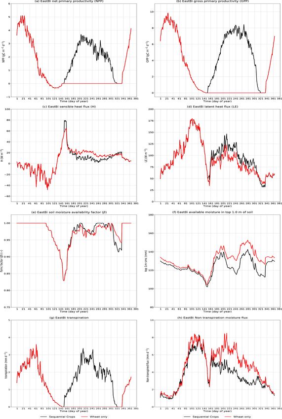
442                         C. Mathison et al.: Implementation of sequential cropping into JULESv5.2 land-surface model

Table 3. JULES crop parameters used in this study. The sorghum cardinal temperatures are from Nicklin (2012) with the other parameters
being those used for maize in Osborne et al. (2015). We include only the values that have been changed or added since Osborne et al.
(2015). Table 3 of Osborne et al. (2015) provides the original PFT parameters and Table 4 of Osborne et al. (2015) provides the original crop
parameters.

         Parameter        JULES                  Description (units)                       Winter    Sorghum      Spring       Rice
                          notation                                                         wheat                   wheat
         Tb               t_bse_io               Base temperature (K).                     273.15      284.15     273.15     278.15
         Tm               t_max_io               Max temperature (K).                      303.15      317.15     308.15     315.15
         To               t_opt_io               Optimum temperature (K).                  293.15      305.15     293.15     303.15
         TTemr            tt_emr_io              Thermal time between sowing and               35          80         35         60
                                                 emergence (degree days).
         TTveg            tt_veg_io              Thermal time between emergence and       Table 4      Table 4   Table 5    Table 5
                                                 flowering (degree days).
         TTrep            tt_rep_io              Thermal time between flowering and       Table 4      Table 4   Table 5    Table 5
                                                 maturity (degree days).
         Tmort            t_mort_io              Soil temperature (second level) at        273.15      281.15     273.15     281.15
                                                 which to kill crop if DVI > 1 (K).
         fyield           yield_frac_io          Fraction of the harvest carbon pool          1.0          1.0        1.0        1.0
                                                 converted to yield carbon.
         DVIinit          initial_c_dvi_io       DVI at which the crop carbon is set to       0.0          0.0        0.0        0.0
                                                 Cinit .
         DVIsen           sen_dvi_io             DVI at which leaf senescence begins.         1.5          1.5       1.5        1.5
         Cinit            initial_carbon_io      Carbon in crop at emergence in              0.01         0.01      0.01       0.01
                                                 kg C m−2 .

2.2     Implementing sequential cropping in JULES-crop                   Sequential cropping provides clear added benefits for the fol-
                                                                         lowing reasons:
2.2.1    JULES-crop: rationale for implementing                             – providing a more realistic representation of the observed
         sequential cropping in JULES-crop                                    surface land cover;

                                                                            – allowing the continuous simulation of a location where
JULES-crop is typically run as a single-crop model, rep-
                                                                              different crops are grown within the same area, thereby
resented by the red curve in Fig. 1, where a primary crop
                                                                              simulating water resource demand from crops;
is simulated but no second crop is possible, and the land
is left fallow with a minimum surface cover. In many re-                    – allowing the climate to affect both the water and crops,
gions, sequential cropping is the main cropping system used,                  while simultaneously allowing interactions between
with several crops cultivated one after another. JULES-crop                   water and crops throughout the year makes it possible
has been developed for implementation in Earth system and                     to simulate the integrated impacts of climate change on
climate models for application in adaptation and mitigation                   these two sectors; and
studies. Only being able to simulate one crop per year is
therefore limiting application in many parts of the world. In               – providing the opportunity to investigate the impact of
the changes to JULES described in Sect. 2.2.2, new controls                   adopting sequential cropping for regions where it is not
are implemented to allow the current JULES-crop code to be                    currently used.
run more than once in a year at a particular location, so that
sequential cropping systems can be represented in JULES.                 2.2.2   The sequential cropping method and the
Sequential cropping is available from version 5.7 of JULES;                      modifications made to JULES-crop
this option is represented by the black curve in Fig. 1.
   The implementation of sequential crops in JULES is part               The sequential cropping method implemented into JULES
of a project to develop simulations for South Asia to under-             as part of this study is illustrated by the flowchart in Fig. 2
stand the impacts of climate change on both agriculture and              and described here using the Avignon site simulation. The
water sectors (Mathison et al., 2015, 2018) using existing re-           Avignon site is a point run which is assumed to be entirely
gional climate model (RCM) projections (Kumar et al., 2013;              used to grow sorghum (from spring to late summer) and win-
Mathison et al., 2013). This will improve understanding of               ter wheat (from winter to early summer). JULES updates the
the impacts of climate change and how they affect each other.            fraction of the site that is allocated to sorghum (winter wheat)

Geosci. Model Dev., 14, 437–471, 2021                                                       https://doi.org/10.5194/gmd-14-437-2021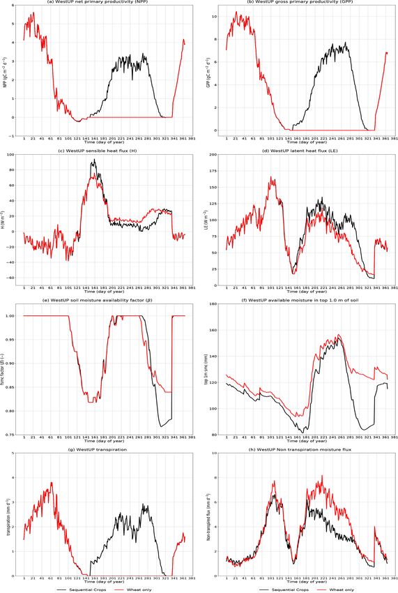
C. Mathison et al.: Implementation of sequential cropping into JULESv5.2 land-surface model                                      443

just before the sowing date so that the appropriate crop oc-          3   Model simulations
cupies the whole of the site. The fraction of the site that is
sorghum (winter wheat) is prescribed in the Avignon case              The description of the simulations is divided into two sec-
using observed sowing and harvest dates. Once the fraction            tions. Section 3.1 describes the Avignon point simulations;
is updated, the crop is sown; it then develops between the            this is a well-observed site used to describe and demonstrate
stages of sowing and emergence, emergence and flowering,              the sequential cropping method and evaluate it against obser-
and flowering and maturity.                                           vations at this location. Avignon is a typical Mediterranean
   In order to simulate the characteristics of a typical se-          crop succession (Garrigues et al., 2015a) characterized by a
quential cropping location using JULES, we made modifi-               succession of winter and summer crops and in between a
cations to both JULES-crop and the irrigation code. To sim-           period of bare soil. When a summer crop follows a winter
ulate crops in sequence on the same grid box, each crop must          crop, the period of bare soil can last up to 9 months. Win-
be completed cleanly so the second one can be sown accord-            ter crops are generally seeded October–November with har-
ingly. The specification of a latest harvest date (latestharvest-     vest towards the end of June–July. Summer crops are seeded
date) forces the harvest of the first crop regardless of whether      in late April–May and harvested at the end of August. Sec-
it has reached maturity or not. The latestharvestdate is a safe-      tion 3.2 describes the simulations of northern India where
guard built into the model, usually set to a date well after the      a more traditional sequential cropping system is commonly
expected harvest date. If the latestharvestdate is used, an alert     used, with a regular rotation between rice during the wetter
is triggered, which provides some initial information to aid          kharif season and wheat during the drier rabi season. The pa-
the investigation of the problem. In this study, the latesthar-       rameter settings and switches used in JULES for the simula-
vestdate is set but never actually required for any of the sim-       tions in this study are provided in Tables 1, 2 and 3. The Avi-
ulations, which is the ideal scenario. The latestharvestdate          gnon and India simulations use the same settings wherever
safeguard is preferable to the simulation of a crop growing           possible; these are provided in Table 1 (see Avignon settings
for an unrealistically long time, i.e. developing too slowly          and India settings columns).
and overlapping the next growing season. This is essential               The PFT parameter settings are also broadly the same be-
for the implementation of sequential cropping at a global or          tween simulations, with the majority of these from Osborne
regional scale, where the model is forced to grow crops that          et al. (2015) and therefore based on natural grasses. The
are potentially unsuitable for a particular grid box. This is         crops are different between the two sets of simulations with
more likely for global simulations, which typically simulate          winter wheat and sorghum at the Avignon site and spring
a restricted set of crop types and varieties. These modifica-         wheat and rice at the India locations. The PFT parameters
tions are controlled using the l_croprotate switch (Table 1).         used in this study that govern Vcmax : including the lower
Therefore, l_croprotate ensures the following:                        (Tlow ) and upper (Tupp ) temperatures for photosynthesis, neff
                                                                      and nl (0) are tuned to the maximum leaf assimilation expres-
  – All crops are initialized at the start of a simulation so         sion from Penning de Vries et al. (1989) for each crop (Ta-
    that they can be used later when they are needed within           ble 2). These values are consistent with the wider literature
    the crop rotation being modelled.                                 (Hu et al., 2014; Sinclair et al., 2000; Olsovska et al., 2016;
                                                                      Xue, 2015; Makino, 2003; Ogbaga, 2014). The parameters
  – If JULES is simulating a crop rotation, the user must             µrl and µsl are the ratios of root-to-leaf and stem-to-leaf ni-
    supply a latestharvestdate so that the first crop is har-         trogen concentrations, respectively; these are tuned to those
    vested before the second crop is sown (a latestharvest-           given in Penning de Vries et al. (1989) to lower the plant
    date can also be specified without using l_croprotate).           maintenance respiration, which was high in some of the ini-
                                                                      tial simulations. The crop parameters are mainly from Os-
   The current JULES default for irrigation allows individ-           borne et al. (2015), with maize parameters used for sorghum
ual tiles to be specified (when frac_irrig_all_tiles is set to        (Sect. 3.1), except for the cardinal temperatures (Table 3)
false) but the irrigation is applied as an average across a           which are from Nicklin (2012).
grid box and therefore actually occurs across tiles. The flag            The calculation of the soil moisture availability factor
set_irrfrac_on_irrtiles restricts the irrigation to the tiles spec-   (beta, β, Table 2) is different between the Avignon and In-
ified by irrigtiles only (Table 1). This new functionality is         dia simulations. β in each layer is 0 below the wilting soil
needed because many locations that include crop rotations             moisture and 1 above a threshold; this is shown in Fig. 1 of
include crops that both do and do not require irrigation.             Williams et al. (2019). In the Avignon simulations, we as-
   The flowchart shown in Fig. 2 is equally applicable to the         sume a rectangular root distribution and the total depth of the
India simulations. Rice is therefore represented by the sum-          root-zone dr to be 1.5 m, equivalent to the observed average
mer crop (green boxes) and wheat is represented by the win-           maximum root depth over all of the years at the Avignon site.
ter crop (purple boxes). This method could be extended to             β is then calculated using this maximum root depth together
include as many crops as those occurring in a rotation at a           with the average properties of the soil. The India single-grid-
particular location.                                                  box simulations assume an exponential root distribution with

https://doi.org/10.5194/gmd-14-437-2021                                                   Geosci. Model Dev., 14, 437–471, 2021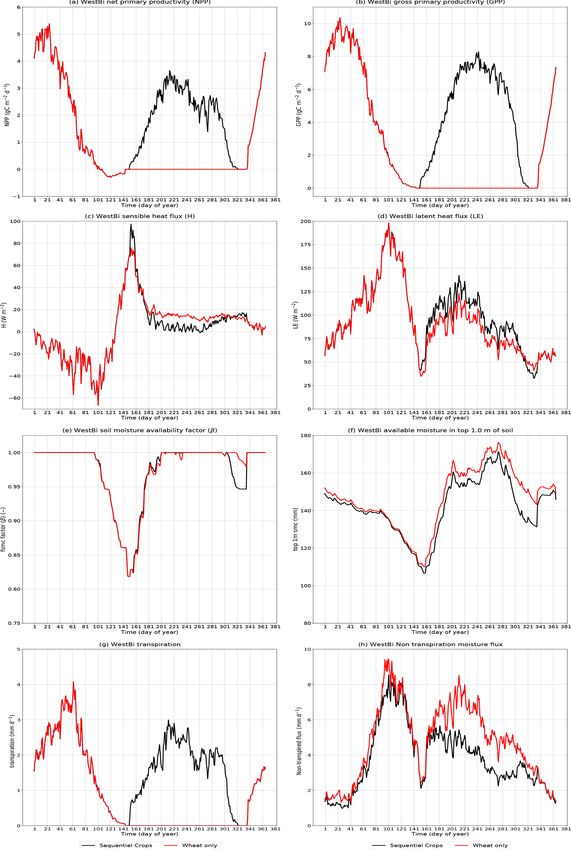
444                        C. Mathison et al.: Implementation of sequential cropping into JULESv5.2 land-surface model

an e-folding depth dr of 0.5 m because we do not have an                The length and detail of the observation record at the Avi-
observed root depth for these locations. In all simulations in       gnon site indicate that it is an ideal site to demonstrate the
this study, we adjust the parameters that affect the use of wa-      method being implemented in JULES for simulating sequen-
ter by the plant so that the plants experience less water stress     tial cropping. High-resolution meteorological data, important
(this parameter is P0 and is set to 0.5; Allen et al., 1998, Ta-     for the practicalities of running the JULES model, are used to
ble 2). This is because water stress is not the main focus of        run the model using a half-hourly time step; this includes air
this analysis, but the representation of soil moisture stress on     temperature, humidity, wind speed, rainfall, radiation mea-
vegetation is a known issue in JULES; this is the subject of a       surements and atmospheric pressure at a height of 2 m above
large international collaborative effort (Williams et al., 2019;     the surface (Garrigues et al., 2015a, 2018). Irrigation in Avi-
Harper et al., 2020). The individual simulations are described       gnon is only applied to the summer crops, i.e. sorghum. The
in more detail in Sect. 3.1 and 3.2 for the Avignon and India        observed irrigation amounts are added to the precipitation
simulations, respectively. The purpose of including Avignon          driving data at the exact day and time they were applied to the
is because it provides a wealth of observations for evaluat-         crops (Garrigues et al., 2015a, 2018). The irrigation and other
ing land-surface models, where there is no equivalent site for       settings governing irrigation are therefore not switched on
South Asia. Observations of these fluxes show if the model           in JULES for the Avignon site simulations (Table 1, column
is correctly representing the fluxes and coverage of the land        “Avignon settings”). We include simulations for the Avignon
surface. The purpose of including a simulation that does not         site where the crops are represented by grasses (Avi-grass)
use the crop model but approximates crops using grasses is           for comparison with the simulations that use the JULES-crop
to show how the model performs with the correct LAI and              model. In the Avi-grass simulations, the LAI and the canopy
height; i.e. it is a clean test of the representation of leaf pho-   height are prescribed from observations in order to capture
tosynthesis, stomatal conductance, water stress and leaf-to-         the growing seasons correctly without the crop model, and
canopy scaling within the model (these parts of the code are         the PFT parameters are adjusted to be the same as the crops.
shared by both natural vegetation and crops).                        These Avi-grass simulations use the same photosynthesis and
                                                                     respiration calculation as JULES-crop, but this is not allowed
3.1   Avignon, France, simulations                                   to influence LAI as they do in the crop model. This allows the
                                                                     evaluation of the photosynthesis and respiration parts of the
The Avignon “remote sensing and flux site” of the National           model, together with the water and energy fluxes, when the
Research Institute for Agriculture, Food and Environment             observed LAI and canopy height are used. In the Avi-grass
(INRAE), described in Garrigues et al. (2015a, 2018), pro-           simulations, JULES is not modelling the crops as grasses
vides a well-studied location (Avignon, France 43.917◦ N             but fixing some parts of the crops (LAI and canopy height)
4.878◦ E) with several years of crop rotation data. The Avi-         straight to observations. We also run two simulations that use
gnon simulations focus on the period between 2005 and 2013           the crop model: a single-crop (Avi-single) and a sequential-
with a rotation of just two crops: winter wheat and sorghum.         crop simulation (Avi-sequential). In both the Avi-single and
JULES already contains parameterizations for wheat and               Avi-sequential simulations, the LAI and the canopy height
maize. The wheat in JULES is the spring variety which                are calculated by the model. The JULES total aboveground
is similar to the winter wheat crop that is grown in Avi-            biomass is calculated from the sum of the stem, leaf and har-
gnon. Spring wheat does not require a vernalization period,          vest carbon pools for each crop. Observed sowing and har-
which is a process usually needed for winter wheat varieties         vest dates from Garrigues et al. (2015a) are used to calculate
to achieve optimum yields (Griffiths et al., 1985; Robert-           the thermal time requirements for each crop represented in
son et al., 1996; Mathison et al., 2018). Vernalization is           the simulations; these are provided in Table 4. During the
not explicitly implemented in JULES; therefore, spring and           periods between each crop, the ground is mostly bare (Gar-
winter wheat can be simulated interchangeably. The maize             rigues et al., 2018). The only difference between the Avi-
crop is a C4 crop that is similar to sorghum. Therefore, we          sequential and Avi-single simulations is that Avi-single only
use these existing parameterizations rather than develop new         simulates wheat; therefore, no sowing dates are provided for
ones. During this period, two varieties of sorghum were cul-         sorghum.
tivated. In 2009, a fodder crop variety was grown, with a
shorter growing season and a larger LAI than the variety for         3.2   Uttar Pradesh and Bihar, India, simulations
the other two years (2007 and 2011). Therefore, the 2009
sorghum crop is planted much later in the year compared              The India simulations focus on the northern Indian states of
to the other two sorghum seasons (2007 and 2011) but har-            Uttar Pradesh and Bihar. These states are key producers of
vested at a similar time. The aim of simulating the crops at         rice and wheat in South Asia and use a regular rice–wheat
this site is to demonstrate the new sequential cropping func-        rotation that is prevalent in this part of India (Mahajan and
tionality in JULES and show how the implementation of se-            Gupta, 2009). We include single-grid-box simulations and
quential cropping affects the JULES crops simulated.                 a regional simulation. The single-grid-box simulations are a
                                                                     selection of four locations from across these two states. For

Geosci. Model Dev., 14, 437–471, 2021                                                  https://doi.org/10.5194/gmd-14-437-2021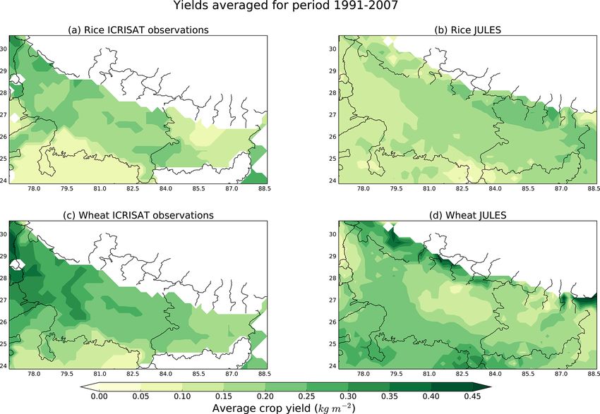
C. Mathison et al.: Implementation of sequential cropping into JULESv5.2 land-surface model                                            445

Table 4. Thermal times in degree days used in this study for the Avignon site; these are based on the observed sowing and harvest dates from
Garrigues et al. (2015a).

   Year       Crop               Sowing date        Harvest date        Emergence – flowering     Flowering – maturity     Sowing DOY
   2005       Winter wheat       27 Oct 2005                                            1301.3                    867.5             300
   2006                                             27 Jun 2006
   2007       Sorghum            10 May 2007        16 Oct 2007                          647.6                    791.5             130
   2007       Winter wheat       13 Nov 2007                                            1401.0                    934.0             317
   2008                                             1 Jul 2008
   2009       Sorghum            25 Jun 2009        22 Sep 2009                          462.5                    565.3             176
   2009       Winter wheat       19 Nov 2009                                            1308.6                    872.4             323
   2010                                             13 Jul 2010
   2011       Sorghum            22 Apr 2011        22 Sep 2011                          679.5                   830.5              112
   2011       Winter wheat       19 Oct 2011                                            1559.6                  1039.7              292
   2012                                             25 Jun 2012

                                                                        that wheat and rice are grown in every grid box across the
                                                                        two states and the crops are not limited by nutrient availabil-
                                                                        ity. The sequential cropping system in this region involves
                                                                        growing rice during the wet monsoon months and an irri-
                                                                        gated wheat crop during the dry winter. In these simulations
                                                                        (both single grid box and regional), wheat is only irrigated
                                                                        during its growing period and without applying limits due to
                                                                        water availability (this is referred to as unlimited irrigation).
                                                                        The wheat variety grown in India is spring wheat, which is
                                                                        the standard variety represented by JULES (Sect. 3.1).
                                                                           The locations of the selected grid boxes are shown on a
                                                                        map of the surface altitude for South Asia in Fig. 3a. The
                                                                        driving data used for these four simulations are from an RCM
                                                                        simulation run for South Asia for the period 1991–2007 as
                                                                        described below. Figure 3b, c and d show a close-up view
                                                                        of the locations selected. The map in Fig. 3b shows the av-
                                                                        erage total monsoon precipitation for the 1991–2007 period,
                                                                        while Fig. 3c and d show the average minimum and maxi-
                                                                        mum temperatures, respectively, to illustrate that these four
                                                                        grid boxes are representative of the climate of the wider Uttar
                                                                        Pradesh/Bihar region.
Figure 1. A schematic describing the single-crop model (red curve)         In both the single-grid-box and regional India simulations,
that is part of the standard JULES-crop and the new option for in-      JULES is run using a 3-hourly time step using driving data
cluding sequential cropping (black curve). This schematic repre-        from ERA-Interim (Dee et al., 2011; Simmons et al., 2007)
sents a generic crop at a single location.                              downscaled to 25 km using the HadRM3 RCM (Jones et al.,
                                                                        2004). This RCM simulation is one of an ensemble of sim-
                                                                        ulations produced for the EU-HighNoon FP7 project for the
each grid box, both single-crop (referred to as India-single)           entire Indian subcontinent (25–32◦ N, 79–88◦ E). The High-
and sequential-crop (referred to as India-sequential) simu-             Noon simulations are described in detail in previous pub-
lations are run. India-single and India-sequential are set up           lications such as Kumar et al. (2013) and Mathison et al.
in the same way, with the only difference being that sow-               (2013, 2015). HadRM3 provides more regional details in ad-
ing dates are provided for just one crop. For consistency               dition to the global data with updated 3-hourly lateral at-
with the rest of the simulations, only wheat is simulated in            mospheric boundary conditions interpolated to a 150 s time
India-single. The single-grid-box simulations enable a simi-            step. These simulations include a detailed representation of
lar analysis to that described for Avignon (Sect. 3.1), while           the land surface in the form of version 2.2 of the Met Of-
the regional simulation (this is only a sequential-crop run)            fice Surface Exchange Scheme (MOSESv2.2; Essery et al.,
is a demonstration of the sequential cropping method being              2001). JULES has been developed from the MOSESv2.2
used at larger scales. For the regional simulation, we assume           land-surface scheme, and therefore the treatment of different

https://doi.org/10.5194/gmd-14-437-2021                                                        Geosci. Model Dev., 14, 437–471, 2021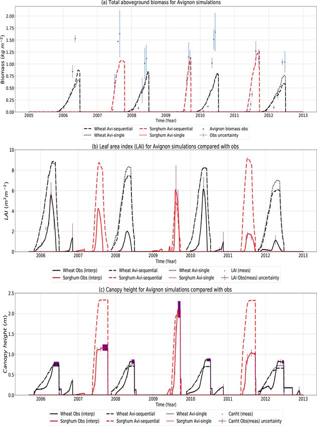
446                         C. Mathison et al.: Implementation of sequential cropping into JULESv5.2 land-surface model

Figure 2. A flowchart showing the sequence followed to carry out the crop rotation in JULES. The first step (top green box) in the sequence
is to update the first crop fraction; this occurs as or just before the first crop is sown.

surface types is consistent between the RCM and JULES (Es-                1. Null hypothesis: the inclusion of a secondary crop on
sery et al., 2001; Mathison et al., 2015). In the India single-              the same field does not change the growth and devel-
grid-box simulations, sowing dates are prescribed using cli-                 opment of the primary crop in an irregular sequential
matologies calculated from the observed dataset (Bodh et al.,                cropping rotation with long fallow periods.
2015) from the government of India, Ministry of Agricul-                     Alternative hypothesis: the inclusion of a secondary
ture and Farmers Welfare. Thermal times are calculated us-                   crop on the same field modifies the growth and devel-
ing these climatological sowing and harvest dates from Bodh                  opment of the primary crop in an irregular sequential
et al. (2015) and a thermal climatology from the model sim-                  cropping rotation with long fallow periods.
ulation as described in Osborne et al. (2015); the values used
in the simulations here are provided in Table 5. In the re-               2. Null hypothesis: the inclusion of a secondary crop on
gional simulation, the thermal time requirements are esti-                   the same field does not change the energy and carbon
mated from the sowing and harvest dates provided by the                      fluxes in an irregular sequential cropping rotation with
Mathison et al. (2018) method to avoid problems with miss-                   long fallow periods.
ing observed data. The settings used for the India simulations               Alternative hypothesis: the inclusion of a secondary
are provided in Table 1 (column “India settings”). Plots of the              crop on the same field modifies the energy and carbon
regional ancillaries for each of rice and wheat are provided                 fluxes in an irregular sequential cropping rotation with
in Appendix C.                                                               long fallow periods.

                                                                          3. Null hypothesis: in a regular rotation without long fal-
4   Model evaluation                                                         low periods, the inclusion of a secondary crop on the
                                                                             same field does not change the crop development of the
The objectives of this study are to evaluate the model against               primary crop or the grid box energy and carbon fluxes
observations where they are available, for the Avignon point                 and soil conditions.
and the India single-grid-box simulations, and to test the fol-              Alternative hypothesis: in a regular rotation without
lowing hypotheses with regard to the implementation of the                   long fallow periods, the inclusion of a secondary crop
presented sequential cropping method in JULES:                               on the same field modifies the crop development of the

Geosci. Model Dev., 14, 437–471, 2021                                                      https://doi.org/10.5194/gmd-14-437-2021
C. Mathison et al.: Implementation of sequential cropping into JULESv5.2 land-surface model 447
Figure 3. A map showing the location of the single-grid-box simulations in the wider context of India on a map of the surface altitude (a)
from the regional climate model that is used in the JULES simulations. The same locations are shown in three smaller maps (b–d) that zoom
in on the states of Uttar Pradesh and Bihar. The map in panel (b) shows the total monsoon precipitation, (c) shows the minimum temperature,
and (d) shows the maximum temperature averaged for the period 1991–2007.
Table 5. The sowing day of year (sowing DOY) and thermal times in degree days used in this study for the locations in Uttar Pradesh and
Bihar, India (Fig. 3 for a map of the locations), the values given here are based on the observed sowing and harvest dates from Bodh et al.
(2015).
Location Crop Sowing DOY Emergence – flowering Flowering – maturity
WestUP Spring wheat 335 1007.6 671.1
Rice 150 1759.4 1181.3
EastUP Spring wheat 335 993.55 662.5
Rice 150 1865.5 1243.5
WestBi Spring wheat 335 991.54 661.6
Rice 150 1907.55 1271.7
EastBi Spring wheat 335 1019.21 679.1
Rice 150 1976.96 1300.64
https://doi.org/10.5194/gmd-14-437-2021 Geosci. Model Dev., 14, 437–471, 2021448 C. Mathison et al.: Implementation of sequential cropping into JULESv5.2 land-surface model
Table 6. Table of statistics comparing the Avignon simulations with observations for each type of run: Avi-single (single), Avi-sequential
(sequential) and Avi-grass (without the crop model).
Variable Simulation type RMSE Bias r value
GPP (g C m−2 d−1 ) grass 2.0 −1.0 0.95
sequential 3.0 0.0 0.82
single 5.0 −2.0 0.52
H (W m−2 ) grass 37.0 13.0 0.76
sequential 38.0 6.0 0.71
single 39.0 11.0 0.71
LE (W m−2 ) grass 28.0 −3.0 0.81
sequential 33.0 0.0 0.73
single 37.0 −8.0 0.64
primary crop, the grid box energy and carbon fluxes and eral years (2001 to 2014), growing a range of crops through-
soil conditions. out this period. No equivalent site to Avignon has been found
for South Asia.
The first set of hypotheses will be assessed by compar- The observations for evaluating the model include canopy
ison of the observed LAI, canopy height and total above- height (measured every 10 d), aboveground dry weight
ground biomass in Avignon with single-crop and sequential- biomass (taken at four field locations) and LAI; biomass and
crop simulations. The second set of hypotheses will be as- LAI are destructive measurements repeated up to six times
sessed by comparison of observed fluxes, GPP, latent heat per crop cycle (Garrigues et al., 2015a). H and LE flux
(LE) and sensible heat (H ) in Avignon with single-crop and measurements are available for several years, enabling the
sequential-crop simulations. For the third set of hypotheses, evaluation of the JULES fluxes. Cumulative evapotranspira-
we compare JULES yields with observed yields for single- tion (ET) are derived from the half-hourly LE measurements.
and sequential-crop simulations and analyse the same vari- More information is documented in Garrigues et al. (2015a)
ables as for the first and second sets of hypotheses for four regarding the site and the observations available. These con-
locations across the northern Indian states of Uttar Pradesh tinuous measurements of surface fluxes provided by the Avi-
and Bihar. We also assess if the implementation of sequen- gnon dataset are a unique resource for evaluating LSMs and
tial crops affects the soil moisture in a regular sequential-crop for testing and implementing more irregular crop rotations in
system, which does not have long periods of bare soil. For a LSMs.
regular sequential-crop system without long fallow periods,
changes in soil moisture are more likely to be due to the ef- 4.2 India
fects of sequential cropping and are less likely to be affected
by evaporation from bare soil. More information is provided The four India locations (grid boxes) selected for analysis
about the Avignon site in Sect. 4.1 and the climate across the in this study are shown on a map of South Asia in Fig. 3a
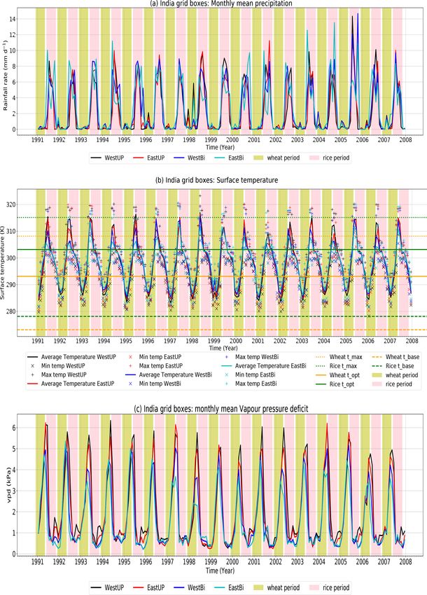
four India grid box locations in Sect. 4.2, including the ob- with smaller inset plots (Fig. 3b, c and d) focusing on the se-
servations used to evaluate the simulations at these locations. quential cropping region being considered across the states
of Uttar Pradesh and Bihar. The climate of this region is
4.1 Avignon summarized in Appendix B (Fig. B1), which shows the time
series of the average precipitation (Fig. B1a), temperatures
Avignon is characterized by a Mediterranean climate with a (Fig. B1b) and vapour pressure deficit (VPD) (Fig. B1c) at
mean annual temperature of 287.15 K (14 ◦ C) and most rain- each of these four grid boxes. The different crop seasons are
fall falling in autumn (with an annual average of 687 mm). emphasized by the different colour shading, with yellow for
The Avignon time series of temperature (with a 10 d smooth- wheat and pink for rice. The temperatures (Fig. B1b) rarely
ing applied) is provided in Appendix A in Fig. A1a and reach the lower cardinal temperatures set in the model (Tb )
precipitation (10 d totals, which include actual irrigation shown for rice (green) or wheat (orange); however, the high
amounts) in Fig. A1b (Garrigues et al., 2015a). In general, temperatures do exceed the maximum cardinal temperatures
Avignon experiences a fairly regular distribution of rainfall (Tm ) for these crops, especially those set for wheat. In gen-
throughout the year and the annual temperature range for eral, EastBi is cooler than the other locations in more of the
Avignon (26 ◦ C) is relatively consistent, with only a brief years, with the two locations in Uttar Pradesh often being
cold snap in early 2012 having a much lower minimum. The the warmest. The precipitation at each location is variable
Avignon site represents the irregular cropping rotation, cho- (Fig. B1a), with variation in the distribution of precipitation
sen because it has been observed and documented over sev- through the monsoon period, which could be important for
Geosci. Model Dev., 14, 437–471, 2021 https://doi.org/10.5194/gmd-14-437-2021C. Mathison et al.: Implementation of sequential cropping into JULESv5.2 land-surface model 449
crop yields. Challinor et al. (2004), for example, found that observations for all four seasons; however, the wheat LAI is
in two seasons with similar rainfall totals, the distribution overestimated. The two wheat seasons of 2006 and 2010 are
of the rainfall during the growing season strongly affected closer to the LAI observations than 2008 and 2012, but the
groundnut crop yield. There is also a clear seasonal cycle underestimation of the biomass is greater for these seasons.
in the VPD, increasing toward the end of the wheat season Garrigues et al. (2015a) highlight that 2006 and 2008 have
and decreasing into the rice season. EastBi generally has the atypical rainfall during the wheat season, with 2006 being
lowest VPD, with WestUP and EastUP usually the highest very dry (256 mm of rain during the wheat season) and 2008
throughout the time series shown (Fig. B1). These time se- being very wet (500 mm during the wheat season). There-
ries show that there is a gradual change in conditions from fore, in 2008, Avignon received 73 % of its annual average
west to east across Uttar Pradesh and Bihar with increasing (Sect. 4.1) during the wheat season alone; these differing
humidity and rainfall and decreasing maximum temperatures conditions could explain the large differences in observed
from west to east. LAI and biomass between the two years (Garrigues et al.,
District-level area and production data from the Interna- 2015a).
tional Crops Research Institute for the Semi-Arid Tropics The shorter observed growing season for the taller fod-
(ICRISAT, 2015) are used to calculate district level yields. der variety of sorghum grown in 2009 can be compared with
These are then gridded at the resolution of the ERA-Interim the longer season, smaller variety grown in 2007 and 2011
data (0.25◦ ) to ensure that the scale of simulated and ob- (solid red line Fig. 4b and c). No sorghum is simulated in
served yields matched. We also show average crop yield ob- Avi-single, so the dotted red line is equal to zero and not
servations for three 5-year periods (Ray et al., 2012a) be- visible in Fig. 4. Avi-sequential (dashed red) simulates the
tween 1993 and 2007 (1993–1997, 1997–2003, 2003–2007). 2009 sorghum season well, in terms of biomass (Fig. 4a),
Data from Ray et al. (2012a) are made available via Ray et al. LAI (Fig. 4b) and canopy height (Fig. 4c); with relatively
(2012b). Ray et al. (2012b) are based on previous publica- small differences between the simulations and observations
tions (Monfreda et al., 2008; Ramankutty et al., 2008). All maximum values (LAI of 1 m2 m−2 and canopy height of
the observations used include the period of the single-grid- 0.1 m). In the 2007 sorghum season, Avi-sequential (dashed
box simulations, which are from the period of 1991–2007. red) overestimates the maximum LAI and canopy height by
We show both of these datasets to highlight that there is a approximately 2 times the observations (Fig. 4b and c) and
range in the estimates of yield for this region. underestimates the total biomass (Fig. 4a) by about 30 %.
For the 2011 season, the Avi-sequential sorghum biomass
is equal to the magnitude of the observations; however, the
5 Results maximum LAI is overestimated by a factor of 4 in the model
(similar to 2007) and the maximum canopy height is approx-
5.1 Evaluation against observations imately 2 times the observed maximum.
The peaks in productivity shown in the LAI in Fig. 4b are
5.1.1 Avignon consistent with the two years (2006 and 2007) of GPP ob-
servations (black line Fig. 5a). The 2006 wheat crop is rep-
Figure 4 shows the time series of total aboveground biomass resented in the GPP of all three simulations, although it is
(a), LAI (b) and canopy height (c) for Avi-sequential and underestimated in all of them (Fig. 5a). The GPP in Avi-
Avi-single compared with observations. The crops in JULES single is lower than both Avi-sequential and Avi-grass dur-
(both single and sequential) are developing throughout the ing the second half of the wheat growing period. The decline
crop seasons, with maxima occurring at approximately the in GPP at the end of the 2006 wheat season is quite close
correct time for the crops being simulated. Therefore, the to the observations for the three simulations, with Avi-grass
lack of vernalization in the model does not affect the simu- (red line) being slightly early and both the crop simulations;
lation of winter wheat in Avignon. Avi-grass simulations are Avi-sequential (blue line) and Avi-single (cyan line) being
not shown, as these follow the observed canopy height and slightly late. For the sorghum growing period, the magnitude
LAI exactly as these values are prescribed in the simulations and timing of the maximum GPP for Avi-sequential (blue
without crops. The total aboveground biomass from JULES line) are a good fit to observations. However, the increase in
is plotted as a time series (dashed lines) for comparison with GPP begins slightly too early for Avi-sequential and slightly
observations, which are provided as a single time series with late for Avi-grass. The Avi-grass simulations slightly under-
the crop type confirmed from the timing of the observations estimate the maximum GPP during the sorghum season and
(purple asterisks in Fig. 4a). The increase in biomass for both it occurs a little later than observed (Fig. 5a). The decline in
crops through the start of the season follows the observations GPP at the end of the sorghum season occurs at the same time
quite closely but in most years, especially for wheat, JULES- as the observations for both Avi-grass and Avi-sequential.
crop (using either single or sequential crops) does not accu- These results are quantified in Fig. A3, with both Avi-grass
mulate enough biomass later in the crop season to reach the (Fig. A3a) and Avi-sequential (Fig. A3b) showing a strong
observed maxima. The wheat canopy height is very close to linear correlation, with r values greater than 0.8. The val-
https://doi.org/10.5194/gmd-14-437-2021 Geosci. Model Dev., 14, 437–471, 2021You can also read


