The ABC-DA system (v1.4): a variational data assimilation system for convective-scale assimilation research with a study of the impact of a ...
←
→
Page content transcription
If your browser does not render page correctly, please read the page content below
Geosci. Model Dev., 13, 3789–3816, 2020
https://doi.org/10.5194/gmd-13-3789-2020
© Author(s) 2020. This work is distributed under
the Creative Commons Attribution 4.0 License.

The ABC-DA system (v1.4): a variational data assimilation system
for convective-scale assimilation research with a study of the impact
of a balance constraint
Ross Noel Bannister
University of Reading, Dept. of Meteorology room 3L62, Meteorology Building, Whiteknights Road,
Earley Gate, Reading RG6 6ET, UK

Correspondence: Ross Noel Bannister (r.n.bannister@reading.ac.uk)

Received: 8 November 2019 – Discussion started: 3 February 2020
Revised: 16 July 2020 – Accepted: 22 July 2020 – Published: 27 August 2020

Abstract. Following the development of the simplified at-       experiments, and it also has associated visualisation soft-
mospheric convective-scale “toy” model (the ABC model,          ware.
named after its three key parameters: the pure gravity wave        As a demonstration, the system is used to tackle a sci-
frequency A, the controller of the acoustic wave speed B, and   entific question concerning the role of geostrophic balance
the constant of proportionality between pressure and density    (GB) to model background error covariances between mass
perturbations C), this paper introduces its associated varia-   and wind fields. This question arises because although GB
tional data assimilation system, ABC-DA. The purpose of         is a very useful mechanism that is successfully exploited in
ABC-DA is to permit quick and efficient research into data      larger-scale assimilation systems, its use is questionable at
assimilation methods suitable for convective-scale systems.     convective scales due to the typically larger Rossby numbers
The system can also be used as an aid to teach and demon-       where GB is not so relevant. A series of identical twin ex-
strate data assimilation principles.                            periments is done in cycled assimilation configurations. One
   ABC-DA is flexible and configurable, and is efficient        experiment exploits GB to represent mass–wind covariances
enough to be run on a personal computer. The system can run     in a mirror of an operational set-up (with use of an additional
a number of assimilation methods (currently 3DVar and 3DF-      vertical regression (VR) step, as used operationally). This ex-
GAT have been implemented), with user configurable obser-       periment performs badly where error accumulates over time.
vation networks. Observation operators for direct observa-      Two further experiments are done: one that does not use GB
tions and wind speeds are part of the current system, and       and another that does but without the VR step. Turning off
these can, for example, be expanded relatively easily to in-    GB impairs the performance, and turning off VR improves
clude operators for Doppler winds. A key feature of any data    the performance in general. It is concluded that there is scope
assimilation system is how it specifies the background error    to further improve the way that the background error covari-
covariance matrix. ABC-DA uses a control variable trans-        ance matrices are represented at convective scale. Ideas for
form method to allow this to be done efficiently. This ver-     further possible developments of ABC-DA are discussed.
sion of ABC-DA mirrors many operational configurations
by modelling multivariate error covariances with uncorre-
lated control parameters, each with special uncorrelated spa-
tial patterns.                                                  1   Introduction
   The software developed performs (amongst other things)
model runs, calibration tasks associated with the background    The grid sizes of limited-area models for operational weather
error covariance matrix, testing and diagnostic tasks, single   forecasting have become small enough to allow some con-
data assimilation runs, and multi-cycle assimilation/forecast   vective processes to be resolved explicitly (Clark et al., 2016;
                                                                Yano et al., 2018). Some leading operational models in-

Published by Copernicus Publications on behalf of the European Geosciences Union.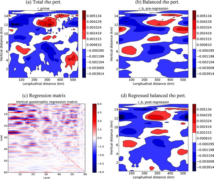
3790                                                                                   R. N Bannister: ABC-DA system v1.4

clude the COSMO (COnsortium for Small-scale MOdelling)            in the B matrix used at the analysis time, the result is often
model (Baldauf et al., 2011), used at MeteoSwiss (1.1 km          corrupted by sampling error due to the small ensemble sizes
grid size) and at the Deutscher Wetterdienst (DWD) (2.8 km        (usually a few tens of members). For this reason, the B ma-
grid size); the AROME (Application of Research to Oper-           trix used operationally is often still modelled according to
ations at Mesoscale) model (Brousseau et al., 2016), used         physical insight. That insight, though, is based on traditional
at Météo-France (1.3 km grid size); the UKV (UK Variable          assumptions of (for instance) geophysical balance, whose ap-
resolution) model (Tang et al., 2013) (1.5 km grid size); and     plicability is questionable at convective scales.
the WRF (US Weather Research and Forecasting) model                  Studying convective-scale DA in operational systems is
(Schwartz and Liu, 2014) (3 km grid size). Each of these sys-     burdened severely by the cost and complexity of these sys-
tems is invaluable in the forecasting of fine-scale weather,      tems. The DA system described in this paper has been de-
including that associated with convective storms, and has its     signed in the same spirit as that of the convective-scale toy
own data assimilation (DA) system to estimate its initial con-    model (the ABC model; Petrie et al., 2017), i.e. with an em-
ditions from new observations and a background state.             phasis on low cost and simplicity. This DA system (together
   Apart from the capability to assimilate new high-              with the model code, hereafter called ABC-DA) is a multi-
resolution observation types, such as radar reflectivity and      featured Var system suited to the ABC model. ABC-DA is
Doppler radial wind, the DA systems are still based on those      actually a suite of software used not only to perform DA it-
designed for use with synoptic- and planetary-scale phenom-       self (in cycling mode if required) but also to calibrate the B
ena in mind. The convective-scale DA problem needs to ac-         matrix from sets of forecast data, to flexibly generate ran-
count for effects that can often be safely ignored or treated     domly perturbed data such as synthetic observations from a
approximately when dealing with large scales. These in-           truth run (which can then be assimilated) to compute a sam-
clude certain dynamical properties of background state errors     ple of covariances implied from a chosen B matrix model and
(namely non-hydrostatic and non-geostrophic contributions,        to perform a set of validation tests. The suite also includes
vertical motion, multiple phases of water, strong inhomo-         sample plotting codes to help visualise and monitor the out-
geneity and flow dependence, and non-Gaussianity), certain        puts, a script to build the executables, sample run scripts,
properties of observation errors (namely cross-correlations),     and detailed user documentation. The ABC-DA numerical
and other features associated with a small grid size (e.g.        codes are written in Fortran 90, scripts are written in Linux
feature misalignment). There are also challenges associ-          Bash, and the plotting code is written in Python 2. Certain
ated with assimilating new observation types (as mentioned        open-source software libraries are also required to compile
above, including the large volumes of data needed), the short     the code.
DA time window (often 1 h or less), the compatibility of lat-        This paper presents the scientific documentation for the
eral boundary conditions from a coarser parent model, and         system, with examples and pointers to how a user can access
questions concerning the appropriateness of allowing DA to        the software. Finally, a short study of ABC-DA is presented
simultaneously modify the larger-scale flows present in the       to investigate the impact of balance constraints in the formu-
convective-scale problem.                                         lation of the convective-scale B matrix. The paper is struc-
   The properties of background state errors are of partic-       tured as follows. In Sect. 2 the ABC model is described, in
ular concern to this paper, although the DA system to be          Sect. 3 the ABC-DA system is outlined, in Sect. 4 the ABC-
described can be equally applied to study other aspects of        DA system is described in detail, in Sect. 5 a brief study of
convective-scale DA, such as the exploration of strategies        the role of geostrophic balance is presented, and in Sect. 6
for high-resolution observation networks (such as those from      the paper is summarised.
Doppler wind instruments), or indeed some of the advanced
DA methods mentioned below. In DA, the background state
is traditionally assumed to be subject to random error, which     2     The ABC model
is distributed according to a Gaussian distribution described
                                                                  2.1    The model equations
by a multivariate error covariance matrix (the “B-matrix”,
e.g. Bannister, 2008a). Given that B is too large to store ex-    The ABC model comprises a set of simplified partial differ-
plicitly, in variational DA (Var) it is represented in the form   ential equations for a two-dimensional spatial grid (x and z)
of a “model” (Bannister, 2008b). One important means of           plus time (t), which are based on the Euler equations. This
representing B in a way that naturally adapts to the flow con-    section summarises the ABC model, and the reader is di-
ditions is to derive a matrix implicitly from an ensemble of      rected to Petrie et al. (2017) for the details. The model equa-
forecasts, which are often produced anyway for probabilis-        tions are as follows:
tic forecasting purposes. This is the basis of the ensemble
Kalman filter (e.g. Houtekamer and Zhang, 2016) and En-
Var (pure ensemble-variational) formulations (e.g. Liu et al.,
2008). Although information from an ensemble in principle
follows the dynamical properties of the model to be reflected

Geosci. Model Dev., 13, 3789–3816, 2020                                           https://doi.org/10.5194/gmd-13-3789-2020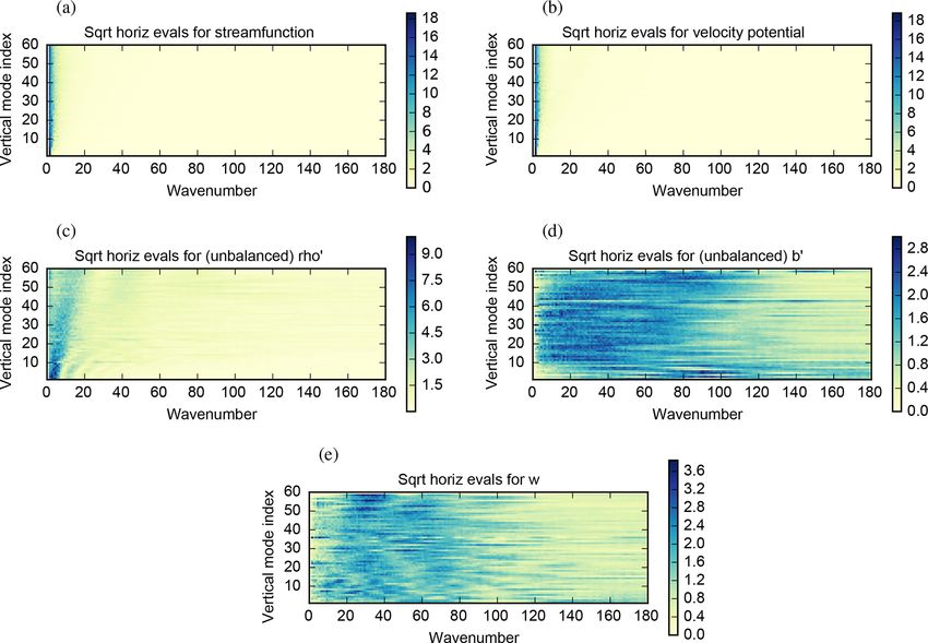
R. N Bannister: ABC-DA system v1.4                                                                                           3791

                                                                    These balance relations are well satisfied for motion at the
                                                                    large scales where Ro is small, and they are used in tradi-
∂u                      ∂ ρ̃ 0
       + Bu · ∇u + C         − f v = 0,                      (1a)   tional Var schemes to model the covariances between mass,
 ∂t                   ∂x                                            wind, and temperature perturbations in background errors.
∂v
       + Bu · ∇v + f u = 0,                                  (1b)   We will revisit these later in the paper.
 ∂t
∂w                     ∂ ρ̃ 0                                       2.3    Discretisation and integration
       + Bu · ∇w + C          − b0 = 0,                      (1c)
 ∂t                    ∂z
∂ ρ̃ 0                                                              As reported in Petrie et al. (2017), the continuous equations
       + B∇ · (ρ̃u) = 0,                                     (1d)   (Eq. 1) have been discretised in time and space; the cur-
 ∂t
∂b0                                                                 rent implementation uses a 360 × 60 (horizontal × vertical)
       + Bu · ∇b0 + A2 w = 0,                                (1e)   element grid with a grid box size of 1500 m × 250 m. Vari-
 ∂t
                                                                   ables are stored on an Arakawa C grid in the horizontal and
where u = u v w is the wind vector (comprising zonal,               Charney–Phillips grid in the vertical (see Fig. 1 of Petrie
meridional, and vertical wind components, respectively); ρ̃         et al., 2017), and periodic boundary conditions are imposed
is the scaled density variable (akin to pressure); b is the         in the horizontal to avoid the need for a driving model to
buoyancy variable (akin to temperature); f is the Cori-             provide lateral boundary conditions. The integration scheme
olis parameter; g is the acceleration due to gravity; and           used is the split-explicit forward–backward scheme of Cullen
A, B, and C are tunable parameters (see below). Primed              and Davies (1991) with a main time step of 1t = 4 s.
variables indicate perturbations from a reference state de-
fined as b(x, z, t) = g+b0 (z)+b0 (x, z, t) and ρ̃(x, z, t) = 1+    2.4    Future developments of the model
ρ̃ 0 (x, z, t). The model supports a range of motions, namely
balanced (Rossby-like) modes and unbalanced (gravity and            The current version of the ABC model does not include
acoustic) modes, which have been studied in detail in Petrie        moist processes. There is much that can be learned about
et al. (2017). There are three tunable parameters: A is the         convective-scale DA from a dry model, but assimilating and
pure gravity wave frequency, controlling the gravity wave           forecasting moisture fields is a major reason for convective-
speeds in the model; B modulates the advective and diver-           scale forecasting (Sun et al., 2014; Bannister et al., 2020).
gent terms in the equations, controlling the acoustic wave          It is planned to upgrade the model to permit the advection
speeds; and C specifies the equation of state that relates pres-    of one or more water variables and allow condensation and
sure and density perturbations, p 0 = Cρ0 ρ̃ 0 , where ρ0 is a      evaporation processes to affect the flow. The assimilation of
density scaling constant. In the linearised equations, only the     moisture is a complex task and so a moist ABC-DA system
product BC (and not B and C individually) affects the char-         is expected to be very useful in that line of research.
acteristics of the flow, so C also controls the acoustic wave
speeds. In numerical integrations of the non-linear equations
(Eq. 1), the effect of scaling C is found to be virtually in-       3     Overview of the ABC-DA system
distinguishable from scaling B in terms of the patterns of
forecast perturbations.                                             Like the ABC model, the DA system is intended to be low
                                                                    cost and easy to run, when compared to a operational-scale
2.2   Properties of the ABC model equations                         system, yet mirror many of the features and options available
                                                                    in operational systems. In this section we review the princi-
Equation (1) conserves total mass and energy, although              ples on which ABC-DA is based, which includes a definition
this exact property is lost when the equations are discre-          of the mathematical notation, but we leave it to Sect. 4 to
tised for numerical integration. The equations approximate          describe the details.
to geostrophic and hydrostatic balance (GB and HB, re-
spectively) when the Rossby number, Ro = U/f L, is small            3.1    Variational data assimilation
(where U is the characteristic zonal wind speed and L is the
characteristic horizontal length scale of the motion). The GB       Var systems construct a scalar functional (called a cost func-
relations are                                                       tion, J ) that is minimised with respect to the state x by con-
            ∂ ρ̃ 0                                                  sidering observations made over a time window (indicated
−fv+C              = 0,                                     (2a)    by an integer time index) t ∈ [0, T ]:
            ∂x
u = 0,                                                      (2b)            1
                                                                    J [x] = (x − x b )B−1 (x − x b )
and the HB relation is                                                      2
                                                                               T
          ∂ ρ̃ 0                                                            1X                   T
                                                                                   y(t) − y m (t) R−1   y(t) − y m (t) .

−b0 + C          = 0.                                        (3)          +                          t                         (4)
          ∂z                                                                2 t=0

https://doi.org/10.5194/gmd-13-3789-2020                                              Geosci. Model Dev., 13, 3789–3816, 2020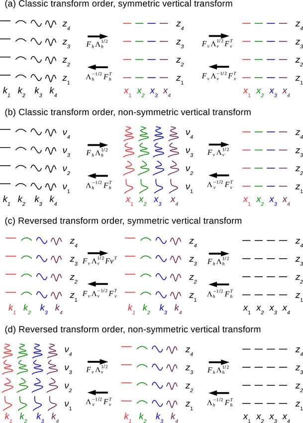
3792                                                                                        R. N Bannister: ABC-DA system v1.4

In Eq. (4), x represents all variables of the model state at       down into a sequence of quadratic problems by iteratively
t = 0 (here u, v, w, ρ̃ 0 , and b0 ) at each location in the do-   linearising M0→t and Ht . This is incremental Var (Courtier
main, x b is a special state at t = 0 called the background        et al., 1994).
state (normally a short forecast from the previous DA), y(t)           Suppose that x r (t) is a reference trajectory satisfying
is the collection of observations at time t, and y m (t) is the    x (t) = Mt−1→t (x r (t − 1)), 1 ≤ t ≤ T . A perturbation to
                                                                     r

model’s version of the observations computed from x. Let           this trajectory (δ prefix) at t is approximately related to
there be n elements in x and pt elements in y(t). Here we          a perturbation at t − 1 via the linear operation δx(t) ≈
use the convention that quantities like x without a time argu-     Mt−1→t δx(t − 1), where the full states are x(t) ≈ x r (t) +
ment imply the value at t = 0. The model’s observations are        δx(t) and x(t − 1) ≈ x r (t − 1) + δx(t − 1). Mt−1→t is the
found in two steps. Firstly, the state is found at time t using    tangent linear (or Jacobian) of Mt−1→t and is mathemat-
the model propagator: x(t) = M0→t (x), which is the result         ically representable by an n × n matrix. We assume that
of integrating Eq. (1) from times 0 to t, and then the model’s     x r (t) + δx(t) is close to Mt−1→t (x r (t − 1) + δx(t − 1)),
observations are found using the observation operator at this      provided that δx(t − 1) is sufficiently small. Similarly, we
time: y m = Ht (x(t)). This DA method is known as 4DVar            suppose that the observation values computed from x r (t) sat-
(Dimet and Talagrand, 1986). B and Rt are covariance matri-        isfy y mr (t) = Ht (x r (t)). A perturbation to these reference
ces (e.g. Kalnay, 2002) pertaining to errors in the background     observations is approximately related to a perturbation in
state and in the observations at time t, respectively. Mathe-      x r (t) via the linear operation δy(t) = Ht δx(t). Ht is the tan-
matically B (an n × n matrix) and Rt (a pt × pt matrix) may        gent linear (or Jacobian) of Ht and is mathematically repre-
be thought as the metrics in which deviations are measured         sentable by a pt × n matrix. These approximations may be
in the cost function (i.e. measures of the precision to which      summarised as the following:
the background and observations are known). The analysis
x a is the special state that minimises J .                        x ≈ x r + δx,                                                (5a)
   The B and Rt matrices are important as they can have a           m          mr           m
                                                                   y (t) ≈ y (t) + δy (t),                                      (5b)
profound effect on the way that observations combine with
the background to yield the analysis. It is a particular chal-     where
lenge to use a B matrix that is relevant to the uncertainties
in convective-scale forecasts. As B is usually a much larger       δy m (t) = Ht M0→t δx.                                       (5c)
matrix than Rt (operationally by orders of magnitude), it can-
                                                                   When Eq. (5) and the following definitions,
not practically be stored explicitly. Instead the B matrix is
modelled, which is usually done via the technique of control       δx b = x b − x r ,                                           (6a)
variable transforms (CVTs) – see Sect. 3.4. As this modelling                                      r
                                                                                                                   mr
                                                                   d(t) = y(t) − Ht M0→t x                  = y(t) − y (t),     (6b)
process is a major component of any DA system, and may re-
quire new thinking for convective-scale systems, much of the       are substituted into Eq. (4), J becomes a functional of the
design of ABC-DA is concerned with how B is modelled. As           perturbation δx instead of the full state x:
a starting point for ABC-DA, the approach that is currently
implemented is a conventional one (to mirror typical current                 1          T
operational configurations that were designed around global        J [δx] =     δx − δx b B−1 δx − δx b
                                                                             2
systems, Sect. 4.2, but still applied for convective-scale sys-                 T
tems). This approach, though, can be adapted to accommo-                     1X
                                                                           +       [Ht M0→t δx − d(t)]T R−1
                                                                                                         t [Ht M0→t δx − d(t)] .
date new convective-scale strategies that are discussed at the               2 t=0
end of the paper.                                                                                                                (7)

3.2    The incremental formulation of the problem                  This is the incremental form of 4DVar. J [δx] is exactly
                                                                   quadratic, allowing efficient algorithms to be used to min-
If M0→t and Ht are linear functions, then Eq. (4) is a             imise it to yield the special state δx a . The iterations required
quadratic function of x and may be minimised using effi-           to minimise Eq. (7) form an inner loop. The full cost func-
cient algorithms such as a conjugate gradient-based method         tion (Eq. 4) is minimised by updating the reference state,
(Golub and Van Loan, 1996; Lewis et al., 2006). The model          x r → x r +δx a , and repeating the inner loops. These iterations
M0→t , though, is a non-linear operator, and many observa-         form the outer loop. In the first outer loop, x r is typically
tions require non-linear observation operators (such as mea-       set to x b . This inner and outer loop procedure, though, does
surements of wind speed, top-of-atmosphere radiance, etc.).        not necessarily find the global minimum of Eq. (4), which
This leads to a non-quadratic function, which may have mul-        can lead to complications in highly non-linear systems with
tiple minima. Furthermore, there are no general efficient min-     a long DA time window (e.g. Fabry and Sun, 2010).
imising algorithms for such problems. In order to simplify             Because M0→t is a difficult operator to derive, the ap-
the problem, the cost function is minimised by breaking it         proximation that M0→t = I is often made. This leads to an

Geosci. Model Dev., 13, 3789–3816, 2020                                                 https://doi.org/10.5194/gmd-13-3789-2020
R. N Bannister: ABC-DA system v1.4                                                                                            3793

approximate method called 3DFGAT (3DVar First Guess at             Notice that the B matrix has effectively disappeared from this
Appropriate Time; Lee et al., 2004; Lawless, 2010). For ap-        formulation because of the assumed statistical properties of
plications when it is too expensive to use M0→t in the DA          δχ . This is a considerable simplification, although the prob-
loops, a further approximation is made that x(t) = x over the      lem of defining the CVT remains. The δχ cost function is
window. This is called 3DVar, although many systems that           minimised (giving the special vector δχ a ), which then leads
specify 3DVar actually use 3DFGAT.                                 to δx a via Eq. (8). This is equivalent to minimising Eq. (7)
                                                                   with a background error covariance matrix equal to
3.3   The observations, their operators, and their error
      statistics                                                   Bic = UUT ,                                                 (10)

The observation operator Ht (and Ht ) is built to suit the range   which is known as the implied background error covariance
of observations assimilated. The components of Ht and Ht           matrix. Apart from not needing to know the B matrix ex-
represent the model’s version of the observations. Typical ex-     plicitly, the minimisation problem (Eq. 9) is found to be nu-
amples include simple bi-linear interpolation of grid values       merically better conditioned than Eq. (7), leading to a more
to an observation location, the computation of model wind          efficient and accurate minimisation.
speed as the root of the sum of squares of the wind com-              It is common to work backwards here: first a CVT is pro-
ponents, or the evaluation of top-of-atmosphere radiance by        posed (based on physical principles such as those discussed
a radiative transfer equation. The ABC-DA system currently         in Bannister (2008b) and later in this paper), and then its abil-
implements observations of the first two kinds, but the system     ity to generate reasonable background error covariance struc-
is flexible enough to support observations of any required         tures is studied by looking at the implied covariances. This
model variable at arbitrary times and positions. The Rt ma-        can be done by studying either UUT or the analysis incre-
trices are taken to be diagonal, and have specified variances.     ments of single-observation DA experiments. Constructing
The system could be adapted to extend any of these aspects         U is one way of doing background error covariance mod-
to include more complicated observation operators, such as         elling. We do this by defining new parameters and their spa-
radiative transfer models, Doppler winds, or for correlated        tial covariances via a proposed form like U = Up Us (Bannis-
observation errors.                                                ter, 2008b). Here Up is the parameter transform (where U−1    p
                                                                   transforms model variables to alternative parameters that are
3.4   Modelling B with control variable transforms                 assumed uncorrelated using sets of balance operators as in
                                                                   Parrish and Derber, 1992; Gauthier et al., 1999), and Us
The B matrix is meant to represent the covariances of errors       is the spatial transform (which transforms each parameter’s
in x b . Operational-scale DA systems all share the challenge      field to modes that are assumed to be uncorrelated, such as
of determining and using B given that this n×n matrix is too       Fourier modes). Us can itself be decomposed into separate
large to manipulate (or even store) and is in any case unknow-     horizontal, vertical, and scaling parts; e.g. Us = 6Uv Uh (see
able. Most practical variational methods use control variable      Sect. 4.2.3). More complicated sequences of transforms are
transforms (CVTs) to simplify this problem. Consider a vec-        also possible, e.g. based on wavelets (Deckmyn and Berre,
tor δχ , which is an alternative representation of δx via the      2005). A property of the CVT approach is that B can be mod-
relation                                                           elled even if it is singular.
δx = Uδχ .                                                  (8)    3.5   The gradient of J and minimising the cost function
δχ is called a control vector, and U is the CVT. The CVT is
                                                                   Equation (7) is minimised by iteratively adjusting δχ until a
a powerful way of accounting for cross-correlations between
                                                                   convergence criterion is met, indicating that a point close to
background errors of model variables (including spatial and
                                                                   the minimum of J [δχ ] has been found. The gradient vector,
multivariate components). δx and δχ have different assumed
                                                                   ∇δχ J , is used with a conjugate gradient algorithm to perform
statistical properties: model space errors have covariance
                                                                   this task. ∇δχ J is found by differentiating J [δχ ]:
 δxδx T b = B, and control variables are taken to be uncorre-
lated and have unit variance δχ δχ T b = I, where the b sub-                                T
                                                                                            X
script indicates expectation over hypothetical background er-      ∇δχ J =δχ − δχ b + UT           MT0→t HTt R−1
                                                                                                              t
ror samples. When Eq. (8) is substituted into Eq. (7), J be-                                 t=0
comes a functional of δχ :                                                  [Ht M0→t Uδχ − d(t)] ,                             (11)
           1           T
                                                                   where d(t) is the difference between the observations at time
J [δχ ] =     δχ − δχ b     δχ − δχ b
           2                                                       t and the model’s version of them based on the reference state
           1X T                                                    Eq. (6b). Equation (11) requires the Jacobians Ht and M0→t ,
        +        [Ht M0→t Uδχ − d(t)]T                             the CVT U, and their adjoint counterparts. The evaluation of
           2 t=0
                                                                   Eq. (11) can be made more efficient by the following stan-
      R−1
       t [Ht M0→t Uδχ − d(t)] .                             (9)    dard algorithm.

https://doi.org/10.5194/gmd-13-3789-2020                                             Geosci. Model Dev., 13, 3789–3816, 2020
3794                                                                                       R. N Bannister: ABC-DA system v1.4

 1. Set the reference state at t = 0 to the background state:     adjoint AT , the adjoint test computes the left- and right-hand
    xr = xb.                                                      sides of the following formula, which must agree to machine
                                                                  precision to gain confidence that the coded adjoint is correct:
 2. Do the outer loop.
                                                                                   ?
       (a) For the first outer loop, δχ b                         (Av in )T Av in = v Tin AT Av in ,                        (12)
                   b      −1   b     r
                                        = 0; otherwise, com-
           pute δχ = U       x −x .
                                                                  where a random vector v in will normally suffice. The CVT
       (b) Compute x r (t) over the time window,                  needs to be inverted in the gradient algorithm when using
           1≤t ≤T,       with       the    non-linear model:      more than one outer loop (step 2a in Sect. 3.5) and in cali-
           x r (t) = Mt−1→t (x r (t − 1)).                        brating the B matrix (Sect. 4.3). These operators are subject
       (c) Compute the reference        state’s   observations:   to an inverse test to demonstrate that the inverse has been
           y mr (t) = Ht (x r (t)).                               coded correctly. This is done by reading in a perturbation
       (d) Compute the differences: d(t) = y(t) − y mr (t).       state and then passing it through AA−1 . The result is out-
       (e) Set δχ = 0 and δx = 0.                                 put, which can be compared to the original field read-in data.
                                                                  A test that the gradient of the cost function (as computed for
       (f) Do the inner loop.                                     the minimisation) is valid can be confirmed in a gradient test,
             i. Integrate the perturbation trajectory over the    which is also provided as part of the test suite. The gradient
                time window, 1 ≤ t ≤ T , with the linear fore-    test estimates progressively more accurate finite-difference
                cast model: δx(t) = Mt−1→t δx(t − 1).             approximations to the gradient, and it checks that they con-
            ii. Compute the perturbations to the model obser-     verge to the analytically computed gradient (Eq. 11). Other
                vations: δy m (t) = Ht δx(t).                     tests are possible that have not been included in this version
                                                                  of ABC-DA, e.g. checks that the innovation statistics, namely
          iii. Compute    1(t) vectors   defined as 1(t) =
                HTt Rt−1 δy m (t) − d(t) .                         (y − y m ) (y − y m )T equals to R + HBic HT (where y m (t) is
           iv. Set the adjoint state λ(T + 1) = 0.                the background’s version of the observations and the angled
            v. Integrate the following adjoint equa-              brackets indicate average over a large number of DA cycles
                tion    backwards       in    time,  T ≥ t ≥ 0:   with the same observation network).
                λ(t) = 1(t) + MTt→t+1 λ(t + 1).
           vi. Compute the gradient as follows: ∇δχ J = δχ −      4     Scientific and technical configuration of ABC-DA
                δχ b + UT λ(0).                                         v1.4
          vii. Use the conjugate gradient algorithm to adjust
                δχ to reduce the value of J .                     This section is a description of the current scientific
         viii. Compute the new increment in model space us-       configuration of the ABC-DA system. This section also
                ing the CVT: δx = Uδχ .                           contains some technical information and can be read in
           ix. Go to step 2fi until the inner-loop convergence    conjunction with the user documentation available on
                criterion is satisfied.                           GitHub (https://github.com/rossbannister/ABC-DA_1.4da/
                                                                  blob/master/docs/Documentation.pdf, last access: 24 Au-
       (g) Update the reference state: x r → x r + δx.            gust 2020) where more information is available, including
       (h) Go to step 2a until the outer-loop convergence cri-    names of the executables to be run, the namelist variables
           terion is satisfied. At convergence, set x a = x r .   that have to be set, and the input and output file names.
                                                                  References are made to this document in the sections below
 3. Run a non-linear forecast from x a for the background of
                                                                  in the form of GitHubDoc§x. The code is divided into master
    the next cycle and longer forecasts if required.
                                                                  programs that perform specific tasks. The relevant variables
The full procedure (adapted for 3DFGAT, where the linear          are set in a namelist file (filenames, options, switches, and
model is omitted) is shown graphically in Sect. 4.7.              parameters), and then the relevant executable is run. A list
                                                                  of the available master routines is listed in GitHubDoc§2,
3.6    System tests                                               and instructions on how to download and build the code are
                                                                  found in GitHubDoc§3.
The system has a special test suite to check aspects of op-
erators that are coded. Operators that have an adjoint coun-      4.1    Construction of a model state and making a
terpart are subject to an adjoint test to demonstrate that the           forecast
adjoint has been coded correctly. This includes the linearised
observation operators and components of U. Many of these          The initial conditions for a model run may be generated
operators are subdivided into constituents that are tested sep-   using the program Master_PrepareABC_InitState (GitHub-
arately (e.g. interpolation, halo swapping, and Fourier trans-    Doc§4.1). The code can take a slice from a specific Met Of-
forms). For a coded operator, A, with input v in and its coded    fice Unified Model (UM) file, or it can generate a simple

Geosci. Model Dev., 13, 3789–3816, 2020                                                https://doi.org/10.5194/gmd-13-3789-2020
R. N Bannister: ABC-DA system v1.4                                                                                                3795

idealised pressure “blob” of specified position and size (or             Note that in Eq. (13) δψ depends only on the merid-
a combination of these). When initial fields are taken from              ional wind and in Eq. (14) δχ vp depends only on the
the UM, they need to be adjusted to make them compati-                   zonal wind. This is unlike a system that has latitude de-
ble with the ABC model. This involves a number of steps:                 pendence, where δψ and δχ vp would each depend on
(i) adjusting the fields towards the E and W edges of the do-            both δu and δv as per the Helmholtz theorem.
main to be consistent with the periodic boundary conditions;
(ii) adding a constant to the v field to force its integral over      3. Compute the GB scaled density:
each level to zero to allow GB in Eq. (2a) (balance condi-                    b
tion, Eq. 2b, though, is not enforced to allow for some im-              δ ρ˜0 = αf δψ/C,                                          (15)
balance); (iii) computing ρ̃ 0 from v with Eq. (2a) and then
                                                                         which follows from application of the Helmholtz the-
adding a constant to force its integral over each level to zero;
                                                                         orem for this system, (δu, δv) = ∂δχvp /∂x, ∂δψ/∂x ,
(iv) computing b0 to satisfy the HB condition (Eq. 3); and
                                                                         applied to the GB equation (Eq. 2a). The value α = 1,
(v) setting w0 so that the 3D winds have zero divergence. A
                                                                         unless the system is configured to turn off GB in this
forecast can be made from these initial conditions using the
                                                                         transform, in which case α = 0.
program Master_RunNLModel (GitHubDoc§4.2) by numer-
ically integrating Eq. (1).                                           4. Compute the balanced scaled density after it has been
                                                                         vertically regressed:
4.2     The CVTs (B matrix) implemented
                                                                              br         b
                                                                         δ ρ˜0 = Rρ δ ρ˜0 .                                        (16)
ABC-DA has a variety of options implemented to model the
B matrix using control variable transforms (CVTs, Sect. 3.4),            The vertical regression (VR) operator Rρ has the form
and this section describes the current implementation. The                          ˜0 ˜0 b
                                                                                             ˜0 b ˜0 b −1             ˜0 b ˜0 b
transforms are most easily understood by describing first the            Rρ = Cδ ρ δ ρ Cδ ρ δ ρ             , where Cδ ρ δ ρ is the cor-
inverse CVTs (since they allow the difference “spaces” to                relation matrix between a previously computed popula-
be defined starting in model space and working towards the                                                                       ˜0 ˜0 b
                                                                         tion of δ ρ˜0 b perturbations with itself, and Cδ ρ δ ρ is the
control space). The CVT operators defined are used in many
                                                                         correlation matrix between δ ρ˜0 b and δ ρ˜0 . The justifica-
of the programs mentioned in later sections.
                                                                         tion for the use of Rρ is given in Appendix B. The sys-
4.2.1    The inverse parameter transform, U−1                            tem can be configured to turn off this step (and is not
                                           p
                                                                         used anyway if α = 0 in step 3).
Recall that U−1p transforms a perturbation in model vari-             5. Compute the unbalanced scaled density:
ables Eq. (1) to alternative parameters that are assumed to
be uncorrelated. It is needed primarily to calibrate the CVT                  u
                                                                         δ ρ˜0 = δ ρ˜0 − δ ρ˜0
                                                                                               br
                                                                                                                                   (17)
(Sect. 4.3). The input fields in this procedure are the pertur-
bations δu, δv, δw, δ ρ˜0 , and δb0 ; the output fields are (in the      (δ ρ˜0 u = δ ρ˜0 if α = 0).
version of the code documented) δψ (streamfunction), δχ vp
                                                                  u   6. Compute the HB buoyancy:
(velocity potential1 ), δ ρ˜0 u (unbalanced scaled density), δb0
(unbalanced buoyancy), and δw u (unbalanced vertical wind).                 b
                                                                         δb0 = βLhb δ ρ˜0 .                                        (18)
All input and output fields are a function of longitude and
height. This is the algorithm for U−1
                                   p .                                   The operator Lhb is defined as Lhb δ ρ˜0 = C∂ ρ̃ 0 /∂z, as in
  1. Compute the streamfunction:                                         Eq. (3). The value β = 1, unless the system is config-
                                                                         ured to turn off HB, in which case β = 0.
      δψ = ∇x−1 δv.                                           (13)
                                                                      7. Compute the unbalanced buoyancy:
      The operator ∇x−1 is defined as ∇x−1 δv =
                                                                             u                b
      (∂/∂x)−2 ∂(δv)/∂x, which is based on application                   δb0 = δb0 − δb0                                           (19)
      of the Helmholtz theorem (see Petrie et al., 2017,                      u
      Sect. 4.1).                                                        (δb0 = δb0 if β = 0).

  2. Compute the velocity potential (again based on the               8. Compute the anelastically balanced vertical wind:
     Helmholtz theorem):
                                                                                             ab ˜0
                                                                         δw b = γ Lab
                                                                                   u δu + Lρ̃ 0 δ ρ .                      (20)
      δχ vp = ∇x−1 δu.                                        (14)
                                                                         Using Eq. (1d), the operators Lab     ab
   1 Do not confuse the velocity potential perturbation, δχ , with                                      u and Lρ̃ 0 are defined
                                                           vp
                                                                         as Lab                   0                    ab ˜0
                                                                                              R
the control vector, δχ.                                                      u δu = −(1/ρ̃0 ) dz ∂(ρ̃0 δu)/∂x and Lρ̃ 0 δ ρ =

https://doi.org/10.5194/gmd-13-3789-2020                                                 Geosci. Model Dev., 13, 3789–3816, 2020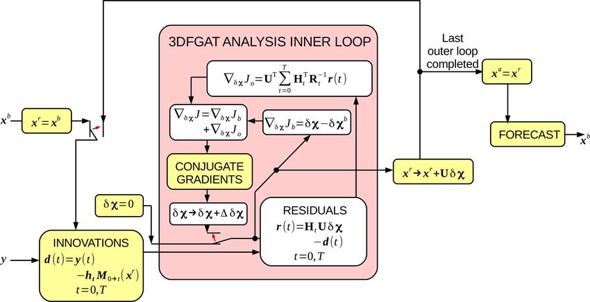
3796 R. N Bannister: ABC-DA system v1.4
−(1/ρ̃0 ) dz0 ∂(u0 δ ρ̃ 0 )/∂x + ∂(w0 δ ρ̃ 0 )/∂z0 (integrat-
R
2. Compute the meridional wind (also based on the
ing from the ground to height z), and δw b is the com- Helmholtz theorem):
ponent of the vertical wind that, with δu, has zero 3D
divergence (sometimes called anelastic balance (AB); δv = ∇x δψ. (24)
see Sect. 3.1.1 of Pielke, 2002). The value γ = 1, un-
less the system is configured to turn off AB, in which 3. Compute the balanced scaled density ρ˜0 b (Eq. 15).
case γ = 0.
4. Compute the vertically regressed balanced scaled den-
9. Compute the unbalanced vertical wind:
sity δ ρ˜0 br (Eq. 16).
δwu = δw − δw b (21)
5. Compute the total scaled density:
(δw u = δw if γ = 0).
br u
Some of these steps may be omitted according to user op- δ ρ˜0 = δ ρ˜0 + δ ρ˜0 . (25)
tions, as specified above. The above steps may be written
b
more compactly as the following “super matrix”: 6. Compute the hydrostatically balanced buoyancy δb0
(Eq. 18).
δχ = U−1 p δx,
7. Compute the total buoyancy:
δψ
δχ vp b u
δ ρ˜0 u =
δb0 = δb0 + δb0 .
δb0 u
8. Compute the anelastically balanced vertical wind δwb
δw u
(Eq. 20).
0 ∇x−1 0 0 0
δu
∇x −1 0 0 0 0 9. Compute the total vertical wind:
δv
f −1
0 −αRρ C ∇x 0 1 0 δw .
0 0 0 −βLhb
1
δ ρ˜0 δw = δwb + δw u . (26)
−γ Lab u 0 1 −γ Lab
ρ̃ 0 0 δb0
Again, some of these steps may be omitted according to user
(22)
options, as set out in Sect. 4.2.1. The above steps may be
It is noted here that this particular form of transform is not written more compactly as the super matrix:
necessarily the most appropriate form for convective-scale
systems, e.g. GB in step 3 and HB in step 6 may not be rele- δx = Up δχ ,
vant. There is, however, expected to be some GB at the larger
δu
scales represented and HB at even shorter scales. Further- δv
more these relationships are still used in some operational
δw =
systems, so their inclusion in this study is justified. The use
δ ρ˜0
of other balance relationships is possible, including statis-
δb0
tical balance relationships (e.g. Derber and Bouttier, 1999;
0 ∇x 0 0 0
Chen et al., 2013; Bannister et al., 2020). An alternative bal- δψ
∇ 0 0 0 0
ance relationship that may be applicable at convective scale δχ vpu
x
αγ Lab R f γ Lab γ Lab 0 1 ˜
is mentioned in the summary. ρ̃ ρ C
0 u ∇x ρ̃ 0
0
δρ . (27)
f 0 u
αRρ C 0 1 0 0 δb
4.2.2 The forward parameter transform, Up hb f δw u
αβL Rρ C 0 βLhb 1 0
Up transforms perturbations of parameters to model space.
This transform (and its adjoint) is used at each iteration of Using Eqs. (22) and (27), it may be confirmed that Up U−1
p =
the Var algorithm. The input fields in this procedure are the I. The adjoint of Eq. (27) is constructed directly from the
u code.
parameter field perturbations δψ, δχ vp , δ ρ˜0 u , δb0 , and δwu ;
the output fields are δu, δv, δw, δ ρ˜0 , and δb0 . This is the 4.2.3 The inverse spatial transform, U−1
s
algorithm for Up .
In the current configuration, the spatial transform comprises
1. Compute the zonal wind based on the Helmholtz theo-
separate horizontal (Uh ), vertical (Uv ), and scaling (6) trans-
rem:
forms. The order of these transforms may vary. The first or-
δu = ∇x δχ vp . (23) dering is called the “classic transform order” (CTO, since
Geosci. Model Dev., 13, 3789–3816, 2020 https://doi.org/10.5194/gmd-13-3789-2020
R. N Bannister: ABC-DA system v1.4                                                                                            3797

this was the transform order in the first Met Office Var sys-        – For the horizontal transform U−1 h , F is called Fh , whose
tem; Wlasak and Cullen, 2014),                                         columns comprise horizontal
                                                                                               √        plane  waves of the form
                                                                       ∼ exp ikx, where i = −1 and k is the wavenumber
      −1 −1 −1
U−1
 s = Uh Uv 6 ,                                             (28)        (each column of Fh is a different k). In this context, FTh
                                                                       represents a horizontal Fourier transform. This makes
and the second is called the “reversed transform order”                the assumption that the eigenvectors of the horizontal
(RTO)                                                                  covariance matrix are plane waves, and the eigenvalues
      −1 −1 −1
                                                                       in 3h are their variances. This is equivalent to assum-
U−1
 s = Uv Uh 6 .                                             (29)        ing horizontal error covariances that are homogeneous
                                                                       (see Bartello and Mitchell, 1992; Berre, 2000; Bannis-
6 is a diagonal matrix of background error standard devia-             ter, 2008b). G is set to I in the horizontal transform.
tions of the parameters, as a function of longitude and height
(although options are implemented to allow the standard de-          – For the vertical transform U−1  v , F is called Fv whose
viation to be a function of height only or a constant for each         columns are the eigenmodes of a vertical covariance
parameter). After the parameters have been divided by 6, the           matrix (labelled with ν; see below), and 3v represents
problem remains one of modelling the covariances between               their variances. G is set either to Fv to give a symmetric
spatial points in space.                                               vertical transform or to I, depending on user choice.
   There are separate spatial operators for each parameter de-
fined in Sect. 4.2.1, and so strictly we should define the over-      The spaces that these operators work in depends on the
all spatial transforms as block-diagonal forms, but we instead     chosen order of the transforms and on whether the vertical
adopt a casual way of describing the transforms to avoid get-      transform is symmetric or not. The following summarises
ting bogged down in notation. Depending on the context,            these options, is repeated for each parameter, and can be read
these transforms may represent all parameters at once (as          with Fig. 1, which shows how the transforms change the hor-
done in Sect. 3.4), single parameters or to individual hori-       izontal and vertical co-ordinates.
zontal levels or vertical columns (as is done below).                – For the CTO, U−1 v operates vertically on a field that is a
   Uh and Uv have the same generic form, as follows:                   function of x and z. The vertical eigenvectors or values
                                                                       are those of a pre-computed horizontally averaged verti-
U−1
 h/v = G3
          −1/2 T
              F ,                                         (30a)        cal covariance matrix, and so these matrices themselves
so Uh/v = F31/2 GT ,                                      (30b)        are not dependent on horizontal position in ABC-DA.

where F is the (exact or assumed) matrix of eigenvectors                  – For the symmetric vertical transform option, U−1  v =
                                                                                 −1/2
(columns of F) of the covariance matrix that is being mod-                  Fv 3v FTv ; the output of U−1  v   is also a field that
elled, 31/2 is the diagonal matrix of eigenvalues, and G is                 is a function of x and z. The horizontal transform,
any orthonormal square matrix (GT G = I) of the same di-                    U−1
                                                                              h , then operates horizontally on such a field. The
mensions as 31/2 . In Eq. (30a), FT projects a state onto the               horizontal eigenvalues are those of pre-computed
eigenvectors (mutually uncorrelated by definition), 3−1/2                   horizontal covariance matrices (one for each z in
scales the projections so they have unit variance, and G is                 ABC-DA). The output of U−1     h is a field that is a
an arbitrary rotation. If the complete CVT had this form (but               function of k and z (see Fig. 1a). This combination
also incorporating 6), then the implied covariance would, by                of options allows a different horizontal covariance
Eq. (10), be                                                                to be specified for each vertical level.
                  T                                                     – For the non-symmetric vertical transform option,
                                                                                       −1/2 T
6F31/2 GT 6F31/2 GT =                                                       U−1
                                                                              v = 3v        Fv ; the output of U−1
                                                                                                                v is a field that is
                                                                            a function of x and vertical eigenmode index ν. The
6F31/2 GT G31/2 FT 6 = 6F3FT 6,                                             horizontal transform, U−1  h , then operates horizon-
                                                                            tally on such a field. The horizontal eigenvalues are
where F3FT is the eigenvalue decomposition of the covari-                   those of pre-computed horizontal covariance matri-
ance matrix in question. In this illustration, the CVT is an                ces (one for each ν in ABC-DA). The output of U−1    h
exact representation of the covariances, but when this proce-               is a field that is a function of k and ν (see Fig. 1b).
dure is applied in practice, it is only an approximate covari-              This combination of options allows a different hor-
ance model, e.g. due to the separation of the horizontal and                izontal covariance to be specified for each vertical
vertical transform or to the application of approximate eigen-              mode, effectively allowing horizontal and vertical
vectors. The structure of the actual implied covariances can                length scales to be associated.
be investigated with the software suite (Sect. 4.4).
   In the ABC-DA system, we use the following for F and G            – For the RTO, U−1 h operates horizontally on a field that
in Eq. (5).                                                            is a function of x and z. The horizontal eigenvalues are

https://doi.org/10.5194/gmd-13-3789-2020                                             Geosci. Model Dev., 13, 3789–3816, 2020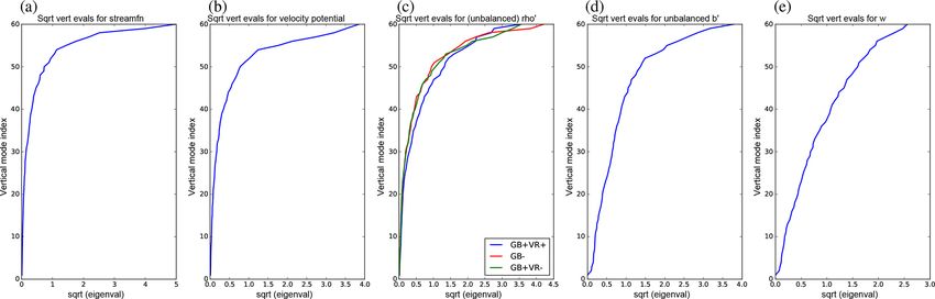
3798                                                                                           R. N Bannister: ABC-DA system v1.4

                                                                          We would expect no difference between the implied covari-
                                                                          ances of the symmetric and non-symmetric vertical trans-
                                                                          form options in the reversed case; although, both options ex-
                                                                          ist in the code.

                                                                          4.2.4    The forward spatial transform, Us

                                                                          The forward spatial transforms follow in a straightforward
                                                                          way from the inverses defined in Sect. 4.2.3, namely for the
                                                                          CTO

                                                                          Us = 6Uv Uh ,                                            (31)

                                                                          and for the RTO

                                                                          Us = 6Uh Uv .                                            (32)

                                                                          The adjoint operators follow in a straightforward manner.

                                                                          4.3     Calibrating the CVTs (B matrix)

                                                                          The CVTs comprise many sub-matrices that need to be de-
                                                                          termined in a calibration procedure. The operators to be de-
                                                                          termined are the regression operator Rρ (part of the pa-
                                                                          rameter transform mentioned in Sect. 4.2.1 and 4.2.2) and
                                                                          6, 3h , Fv , and 3v (parts of the spatial transforms men-
                                                                          tioned in Sect. 4.2.3 and 4.2.4). The number of pieces of
                                                                          information to be determined in this procedure is explored
                                                                          in Appendix A. These matrices are determined from model
                                                                          training data in five stages, all using the program Mas-
Figure 1. Schema to illustrate the different options for the spatial      ter_Calibration (GitHubDoc§4.4), and they are stored in a
transforms as indicated by the panel titles (these are combinations       covariance file, which is produced by this routine. It is im-
of classic and reversed transform orders and symmetric and non-           possible to use a genuine sample of forecast errors to cali-
symmetric vertical transforms). Representations of the vertical di-       brate the B matrix, so instead we use ensembles of forecast
rection include model levels (labelled with z1 , z2 , etc.) and verti-    perturbations, which are considered proxies of forecast er-
cal modes (ν1 , ν2 , etc.). Representations of the horizontal direc-      ror (Buehner, 2005; Pereira and Berre, 2006). The five cal-
tion include model grid points (x1 , x2 , etc.) and Fourier modes (k1 ,
                                                                          ibration stages are described here, and example outputs are
k2 , etc.). Moving from left to right indicates the forward transform
                                                                          shown for a standard set-up (experiment GB+VR+ to be de-
and from right to left indicates the inverse transform. The horizon-
tal transform is always done independently for each vertical co-          scribed in Sect. 5.1).
ordinate (zi to zi or νi to νi ), and the vertical transform is always
done independently for each horizontal co-ordinate (xi to xi or ki to     4.3.1    Generate a population of training data from UM
ki , as guided by the colours). The co-ordinates used in the control               fields
space in each option are indicated on the leftmost panels.
                                                                          This is calibration run stage 1 (Master_Calibration is run
                                                                          with the namelist variable CalibRunStage set to 1). This takes
     those of pre-computed horizontal covariance matrices                 data from one or more UM files (one or more ensembles of
     (one for each z in ABC-DA). The output of U−1        h is a
                                                                          forecasts) and extracts multiple longitude and height slices
     field that is a function of k and z. The vertical transform,         from these files to construct an effective “super ensemble”.
     U−1
       v , uses a separate set of vertical eigenvectors/values
                                                                          These are each adjusted to make them compatible with the
     for each k.                                                          ABC model (as in Sect. 4.1) followed by a short forecast
                                                                          of specified length (in our examples 1 h). These procedures
        – For the symmetric vertical transform option, the                are intended to give the ensemble members properties of the
          output of U−1
                      v is also a field that is a function of             ABC model rather than the Unified Model from which they
          k and z (see Fig. 1c).                                          came, although the degree to which this has been achieved
        – For the non-symmetric vertical transform option,                is not demonstrated. The super ensemble is output from this
          the output of U−1
                          v is a field that is a function of k            stage. Also specified at this stage are the model parameters
          and ν (see Fig. 1d).                                            (in the example to be described A = 0.02 s−1 , B = 0.01, and

Geosci. Model Dev., 13, 3789–3816, 2020                                                    https://doi.org/10.5194/gmd-13-3789-2020
R. N Bannister: ABC-DA system v1.4 3799
Figure 2. Plots comparing an example total scaled density perturbation, δ ρ˜0 , with the diagnosed balanced part, δ ρ˜0 b , and showing the effect
of the regression matrix. (a) δ ρ˜0 (output from stage 2 of the calibration procedure), (b) δ ρ˜0 b (diagnosed from the streamfunction as in Eq. 15),
(c) the regression matrix Rρ (found from stage 3), and (d) its effect on δ ρ˜0 b , i.e. δ ρ˜0 br = Rρ δ ρ˜0 b . Note that in panel (c) the lowermost level
corresponds to the top of the matrix.
C = 10 000 m2 s−2 ) and user settings for the transform op- 4.3.2 Generate a population of forecast perturbations
tions mentioned in Sect. 4.2 (here, unless stated otherwise,
the control options use GB (α = 1), Sect. 4.2.1 step 3; VR, This is calibration run stage 2 (Master_Calibration is run
step 4; HB (β = 1), step 6; no anelastic balance (γ = 0), with the namelist variable CalibRunStage set to 2). The fore-
step 8; the CTO, Sect. 4.2.3; non-symmetric vertical trans- casts output from stage 1 are converted to means and per-
form, Sect. 4.2.3; and parameter standard deviations that are turbations from the means. See GitHubDoc§4.4.2, which in-
a function of vertical level only). These are all output in a cludes plotting information.
provisional covariance file (netCDF format). At this stage,
the file is blank apart from containing information on these 4.3.3 Compute the vertical regression matrix Rρ
options for future reference. These user options are read from
this file in later stages of the calibration when the above men- This is calibration run stage 3 (Master_Calibration is run
tioned matrices are computed and output to this covariance with the namelist variable CalibRunStage set to 3). The per-
file. Technical information is given in GitHubDoc§4.4.1, and turbations from stage 2 are used to calculate populations of
the ensemble members can be plotted using the Python pro- δ ρ˜0 b (Eq. 15). The vertical correlations between δ ρ˜0 b and it-
gram specified there. self and between δ ρ˜0 and δ ρ˜0 b are then used to compute Rρ
In this paper, a super ensemble of 260 members is used. in the way specified in point 4 of Sect. 4.2.1 (see also Ap-
Appendix A shows that this is more than adequate to deter- pendix B). Rρ is then output to the covariance file created in
mine the spatial transform matrices and the vertical regres- stage 1. See GitHubDoc§4.4.3, which includes plotting in-
sion matrix. formation.
Fig. 2a and b compare example δ ρ˜0 and δ ρ˜0 b fields. The
large-scale pattern of these fields is similar, with δ ρ˜0 b be-
ing smoother and of lower magnitude than δ ρ˜0 , indicating
https://doi.org/10.5194/gmd-13-3789-2020 Geosci. Model Dev., 13, 3789–3816, 20203800 R. N Bannister: ABC-DA system v1.4
Figure 3. Profiles of background error standard deviations for the five control parameters with height: (a) streamfunction δψ, (b) velocity
u
potential δχ vp , (c) unbalanced scaled density δ ρ˜0 u , (d) unbalanced buoyancy δb0 , and (e) vertical wind δw. The blue lines are for the
experiment described in the text – namely GB and VR are switched on in the parameter transform. In panel (c) the red line is for the
experiment with GB (and hence VR) switched off, and the green line is for the experiment with GB switched on and VR switched off. In the
other panels all experiments yield the same profiles. The values have been smoothed using a running average over the nearest five levels.
that the unbalanced contributions to δ ρ˜0 are at smaller scales 13 or 14 km for instance does not lie in the ABC model’s
(as expected). Panel (c) shows an example Rρ matrix and stratosphere, and in any case without radiative forcing in the
panel (d) shows its effect on δ ρ˜0 b , showing its ability to mod- ABC model and an ozone layer, we would not expect signa-
ify values and vertical scales. tures of the stratosphere to be present.
The blue lines in Fig. 4 show the square root of the eigen-
4.3.4 Perform the inverse parameter transform on the values of the vertical covariance matrix (diagonal elements
1/2
forecast perturbations of 3v ).3 We find the vertical covariance matrices of each
parameter over each super ensemble member and over each
This is calibration run stage 4 (Master_Calibration is run longitude. Each y axis in Fig. 4 is the (integer) vertical model
with the namelist variable CalibRunStage set to 4). The per- index. The eigensolver sorts these into ascending value of
turbations from stage 2 are transformed to parameters using eigenvalue, so the physical meaning of the modes can be un-
the procedure represented by U−1 p (Sect. 4.2.1) and then out- clear. For instance, examining the eigenvectors by eye (not
put. The mean states found from stage 2 are also used in some shown), for parameters δψ (panel a), δχ vp (panel b), and
of the calculations; e.g. ρ̃0 is used in step 8 of that procedure.
δ ρ˜0 u (panel c), the vertical modes of low index have vertical
See GitHubDoc§4.4.4, which includes plotting information.
profiles that are generally rapidly oscillating and have more
4.3.5 Calibrate the spatial transforms for each weight in the lower model levels than in the upper ones. As
parameter the vertical mode index increases, the oscillations, become
less rapid and tend to have weight over the entire depth of
This is calibration run stage 5 (Master_Calibration is run the model atmosphere. There is no obvious trend concern-
u
with the namelist variable CalibRunStage set to 5). The per- ing the vertical modes of δb0 (panel d) and δw (panel e).
turbations from stage 4 are used to diagnose the matrices 6, The values in Fig. 4 are of comparable magnitude between
Fv , 3v , and 3h for each of the five control parameters. parameters because the vertical error covariance matrices are
The blue lines of Fig. 3 show the background error stan- formed from the populations after they have been normalised
dard deviations (diagonal elements of 6) for the control ex- with 6 −1 – see Eqs. (31) and (32).
periment described above (see the figure caption for a suc- Calibrating the vertical transform involves (for the CTO)
cinct summary). The parameters show some variability with constructing a single global vertical covariance matrix or
height, although none of the parameters show variations of (for the RTO) constructing one vertical covariance matrix for
6 of orders of magnitude. Note that the heights in the ABC each wavenumber. The eigenvalues and eigenvectors follow
model do not correspond with those in the real atmosphere.2 from this procedure. The eigenvectors of the horizontal co-
The large variability of w (panel e) at model heights around
3 In principle the vertical covariance matrix should actually be
2 This is the case because, for simplicity, the irregularly spaced a correlation (rather than covariance) matrix given that the popula-
UM model levels are assigned new regularly spaced heights in the tions have been divided by 6. Due to the approximations made, the
ABC model when generating training data in Sect. 4.3.1. diagonal elements of this matrix may not be exactly unity.
Geosci. Model Dev., 13, 3789–3816, 2020 https://doi.org/10.5194/gmd-13-3789-2020You can also read