Global emissions pathways under different socioeconomic scenarios for use in CMIP6: a dataset of harmonized emissions trajectories through the end ...
←
→
Page content transcription
If your browser does not render page correctly, please read the page content below
Geosci. Model Dev., 12, 1443–1475, 2019
https://doi.org/10.5194/gmd-12-1443-2019
© Author(s) 2019. This work is distributed under
the Creative Commons Attribution 4.0 License.

Global emissions pathways under different socioeconomic scenarios
for use in CMIP6: a dataset of harmonized emissions trajectories
through the end of the century
Matthew J. Gidden1 , Keywan Riahi1 , Steven J. Smith2 , Shinichiro Fujimori3,4 , Gunnar Luderer5 , Elmar Kriegler5 ,
Detlef P. van Vuuren6 , Maarten van den Berg6 , Leyang Feng2 , David Klein5 , Katherine Calvin2 , Jonathan
C. Doelman6 , Stefan Frank1 , Oliver Fricko1 , Mathijs Harmsen6 , Tomoko Hasegawa4 , Petr Havlik1 , Jérôme Hilaire5,7 ,
Rachel Hoesly2 , Jill Horing2 , Alexander Popp5 , Elke Stehfest6 , and Kiyoshi Takahashi4
1 InternationalInstitute for Applied Systems Analysis, Schlossplatz 1, 2361 Laxenburg, Austria
2 JointGlobal Change Research Institute, 5825 University Research Court, Suite 3500, College Park, MD 20740, USA
3 Kyoto University, 361, C1-3, Kyoto University Katsura Campus, Nishikyo-ku, Kyoto 615-8540, Japan
4 Center for Social and Environmental Systems Research, National Institute for Environmental Studies, 16-2 Onogawa,

Tsukuba, Ibaraki 305-8506, Japan
5 Potsdam Institute for Climate Impact Research, Member of the Leibniz Association, P.O. Box 601203,

14412 Potsdam, Germany
6 PBL Netherlands Environmental Assessment Agency, Postbus 30314, 2500 GH The Hague, the Netherlands
7 Mercator Research Institute on Global Commons and Climate Change (MCC) gGmbH, EUREF Campus 19,

Torgauer Str. 12–15, 10829 Berlin, Germany

Correspondence: Matthew J. Gidden (gidden@iiasa.ac.at)

Received: 25 October 2018 – Discussion started: 9 November 2018
Revised: 22 March 2019 – Accepted: 27 March 2019 – Published: 12 April 2019

Abstract. We present a suite of nine scenarios of future emis-   scenario data products are provided for the CMIP6 scientific
sions trajectories of anthropogenic sources, a key deliverable   community including global, regional, and gridded emissions
of the ScenarioMIP experiment within CMIP6. Integrated           datasets.
assessment model results for 14 different emissions species
and 13 emissions sectors are provided for each scenario with
consistent transitions from the historical data used in CMIP6    1   Introduction
to future trajectories using automated harmonization before
being downscaled to provide higher emissions source spa-         Scenario development and analysis play a crucial role in link-
tial detail. We find that the scenarios span a wide range of     ing socioeconomic and technical progress to potential future
end-of-century radiative forcing values, thus making this set    climate outcomes by providing future trajectories of various
of scenarios ideal for exploring a variety of warming path-      emissions species including greenhouse gases, aerosols, and
ways. The set of scenarios is bounded on the low end by a        their precursors. These assessments and associated datasets
1.9 W m−2 scenario, ideal for analyzing a world with end-of-     allow for wide-ranging climate analyses including pathways
century temperatures well below 2 ◦ C, and on the high end       of future warming, localized effects of pollution emissions,
by a 8.5 W m−2 scenario, resulting in an increase in warm-       and impact studies, among others. By spanning a wide range
ing of nearly 5 ◦ C over pre-industrial levels. Between these    of possible futures, including varied levels of emissions mit-
two extremes, scenarios are provided such that differences       igation, pollution control, and socioeconomic development,
between forcing outcomes provide statistically significant re-   scenarios provide a large multivariate space of potential near-
gional temperature outcomes to maximize their usefulness         , medium-, and long-term outcomes for study by the broader
for downstream experiments within CMIP6. A wide range of         scientific community.

Published by Copernicus Publications on behalf of the European Geosciences Union.
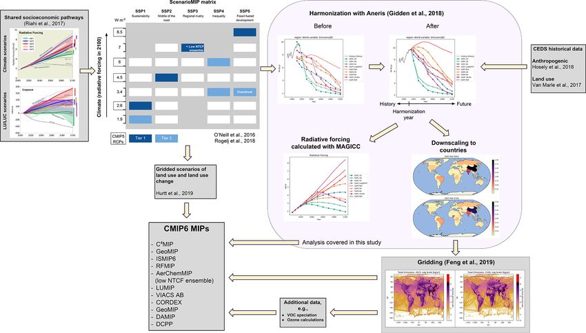
1444                                                        M. J. Gidden et al.: Global emissions pathways for use in CMIP6

   The results of scenario exercises have been used widely by      plement and expand on prior work in CMIP5. While a given
national and international assessment bodies and the global        forcing pathway could be met with potentially many different
scientific community. They have informed previous Assess-          SSPs, a specific SSP is chosen for each pathway according
ment Reports by the Intergovernmental Panel on Climate             to three governing principles: “[maximizing] facilitation of
Change (Solomon et al., 2007; Stocker et al., 2013) as well        climate research, minimizing differences in climate between
as reports on more topical issues including the Special Re-        outcomes produced by the [chosen] SSP, and ensuring con-
port on Emissions Scenarios (SRES) (Nakićenović et al.,          sistency with scenarios that are most relevant to the IAM and
2000). The SRES scenarios were used extensively in the             Impacts, Adaptation, and Vulnerability (IAV) communities”
Coupled Model Intercomparison Project Phase 3 (CMIP3)              (O’Neill et al., 2016, p. 3469).
(Solomon et al., 2007), whereas the following generation of           Selected scenarios sample a range of forcing outcomes
scenarios denoted the “Representative Concentration Path-          (1.9–8.5 W m−2 , calculated with the simple climate model
ways” (RCPs) were used to generate emissions trajectories          MAGICC6; Meinshausen et al., 2011a), with sufficient spac-
in CMIP5 (Moss et al., 2010; van Vuuren et al., 2011; Taylor       ing between forcing outcomes to provide statistically signif-
et al., 2012). These emissions scenarios have been used by a       icant regional temperature outcomes (Tebaldi et al., 2015;
broad audience, including national governments (e.g., Walsh        O’Neill et al., 2016). The nine selected scenarios can be di-
et al., 2014; Hayhoe et al., 2017) and climate scientists (e.g.,   vided into two groups: four scenarios update the RCPs stud-
Kawase et al., 2011; Lamarque et al., 2013; Holmes et al.,         ied in CMIP5, achieving forcing levels of 2.6, 4.5, 6.0, and
2013; Westervelt et al., 2018).                                    8.5 W m−2 , whereas five scenarios fill gaps not previously
   As initially described in Moss et al. (2010), a new frame-      studied in the RCPs, including a lower-bound 1.9 W m−2 sce-
work has been utilized to design scenarios that combine            nario (Rogelj et al., 2018) corresponding to the most op-
socioeconomic and technological development, named the             timistic interpretation of Article 2 of the Paris Agreement
Shared Socioeconomic Pathways (SSPs), with future climate          (United Nations, 2016). Additionally, a new “overshoot” sce-
radiative forcing (RF) outcomes (RCPs) in a scenario matrix        nario is included in the Tier-2 set in which forcing peaks and
architecture (O’Neill et al., 2013; Kriegler et al., 2014; van     then declines to 3.4 W m−2 by 2100 in order to assess the
Vuuren et al., 2013). This new structure provides two criti-       climatic outcomes of such a pathway.
cal elements to the scenario design space: first, it standard-        In order to provide historically consistent and spatially
izes all socioeconomic assumptions (e.g., population, gross        detailed emissions datasets for other scientists collaborat-
domestic product, and poverty, among others) across mod-           ing in CMIP6, scenario results are processed using meth-
eled representations of each scenario; second, it allows for       ods of harmonization and downscaling. Harmonization refers
more nuanced investigation of the variety of pathways by           to the alignment of model results with a common historical
which climate outcomes can be reached. Five different SSPs         dataset. Historical data consistency is paramount for use in
exist, with model quantifications that span potential futures      climate models which perform both historic and future runs,
of green or fossil-fueled growth (SSP1 van Vuuren et al.,          for which there must be smooth transitions between the two
2017, and SSP5 Kriegler et al., 2017), high inequality be-         sets of emissions trajectories. Harmonization has been ap-
tween or within countries (SSP3 Fujimori et al., 2017, and         plied in previous studies (e.g., in SRES – Nakićenović et al.,
SSP4 Calvin et al., 2017), and a “middle-of-the-road” sce-         2000 and the RCPs – van Vuuren et al., 2011; Meinshausen
nario (SSP2 Fricko et al., 2017). For each SSP, a number of        et al., 2011b); however, systematic harmonization for which
different RF targets can be met depending on policies im-          common rules and algorithms are applied across all mod-
plemented, either locally or globally, over the course of the      els has not heretofore been performed (Rogelj et al., 2011).
century (Riahi et al., 2017).                                      We harmonize emissions trajectories, therefore, with a newly
   Scenarios provide critical input for climate models             available methodology and software (Aneris) (Gidden, 2017;
through their description and quantification of both land-use      Gidden et al., 2018) in order to address this need. We fur-
change as well as emissions trajectories. Of the total popu-       ther downscale these results from their native model region
lation of newly available scenarios produced with integrated       spatial dimension to individual countries using techniques
assessment models (IAMs), nine have been chosen for inclu-         which take into account current and future emissions levels
sion for study in ScenarioMIP, one of the dedicated CMIP6-         as well as socioeconomic progress (van Vuuren et al., 2007).
endorsed model intercomparison projects (MIPs) (Eyring             An overview of the scenario selection and processing steps
et al., 2016). The selection of scenarios is designed to al-       that comprise this study as well as its contributions to the
low investigation of two primary scientific questions: “how        broader CMIP6 community is shown in Fig. 1.
does the Earth system respond to climate forcing and how              The remainder of the paper is as follows. First, we discuss
can we assess future climate changes given climate variabil-       scenario selection, historical data aggregation, harmoniza-
ity...and uncertainties in scenarios?” (O’Neill et al., 2016).     tion, and downscaling methods in Sect. 2. We then present
In order to support an experimental design that can address        harmonized model results, focusing on overall emissions tra-
these fundamental questions, scenarios were chosen that ex-        jectories, climate response outcomes, and the spatial distribu-
plore a wide range of future climate forcings that both com-       tion of key emissions species in Sect. 3. Finally, in Sect. 4, we

Geosci. Model Dev., 12, 1443–1475, 2019                                              www.geosci-model-dev.net/12/1443/2019/
M. J. Gidden et al.: Global emissions pathways for use in CMIP6                                                                    1445

Figure 1. The role of ScenarioMIP in the CMIP6 ecosystem. From a population of over 40 possible SSPs, nine are downselected in order to
span the climatic and social dimensions of the ScenarioMIP SSP–RCP matrix. Emissions trajectories developed from these scenarios then
undergo harmonization to a common and consistent historical dataset, downscaling, and gridding. The resulting emissions datasets are then
provided to the CMIP6 scientific community, in conjunction with future scenarios of land use (Hurtt, 2019), concentrations (Meinshausen,
2019), and other domain-specific datasets (e.g., VOC speciation and ozone concentrations).

discuss conclusions drawn from this study as well as guide-            reduced; however, this growth comes at the expense of poten-
lines for using the results presented herein in further CMIP6          tially large impacts from climate change in the case of SSP5.
experiments.                                                           Demand for energy- and resource-intensive agricultural com-
                                                                       modities such as ruminant meat is significantly lower in
                                                                       SSP1 due to changes in behavior and advances in energy effi-
2     Data and methods                                                 ciency. In both scenarios, pollution controls are expanded in
                                                                       high-income economies with other nations catching up rela-
2.1    Socioeconomic and climate scenarios                             tively quickly with the developed world, resulting in reduc-
                                                                       tions in air pollutant emissions. SSP2 is a so-called middle-
The global IAM community has developed a family of sce-                of-the-road scenario with moderate population growth and
narios that describe a variety of possible socioeconomic fu-           slower convergence of income levels across countries. In
tures (the SSPs). The formation, qualitative, and quantitative         SSP2, food consumption, especially for resource-intensive
aspects of these scenarios have been discussed widely in the           livestock-based commodities, is expected to increase and en-
literature (O’Neill et al., 2017; KC and Lutz, 2017; Dellink           ergy generation continues to rely on fossil fuels at approxi-
et al., 2015; Jiang and O’Neill, 2017). We briefly summa-              mately the same rates as today, resulting in continued growth
rize here relevant narratives of the baseline SSPs concern-            of GHG emissions. Efforts at curbing air pollution continue
ing socioeconomic development (see, e.g., Fig. A1), energy             along current trajectories with developing economies ulti-
systems (Bauer et al., 2017), land use (Popp et al., 2017),            mately catching up to high-income nations, resulting in an
greenhouse gas (GHG) emissions (Riahi et al., 2017), and air           eventual decrease in pollutant emissions. Finally, SSP3 and
pollution (Rao et al., 2017).                                          SSP4 depict futures with high inequality between countries
   SSP1 and SSP5 describe worlds with strong economic                  (i.e., “regional rivalry”) and within countries, respectively.
growth via sustainable and fossil fuel pathways, respectively.         Global gross domestic product (GDP) growth is low in both
In both scenarios, incomes increase substantially across the           scenarios and concentrated in currently high-income nations,
globe and inequality within and between countries is greatly

www.geosci-model-dev.net/12/1443/2019/                                                    Geosci. Model Dev., 12, 1443–1475, 2019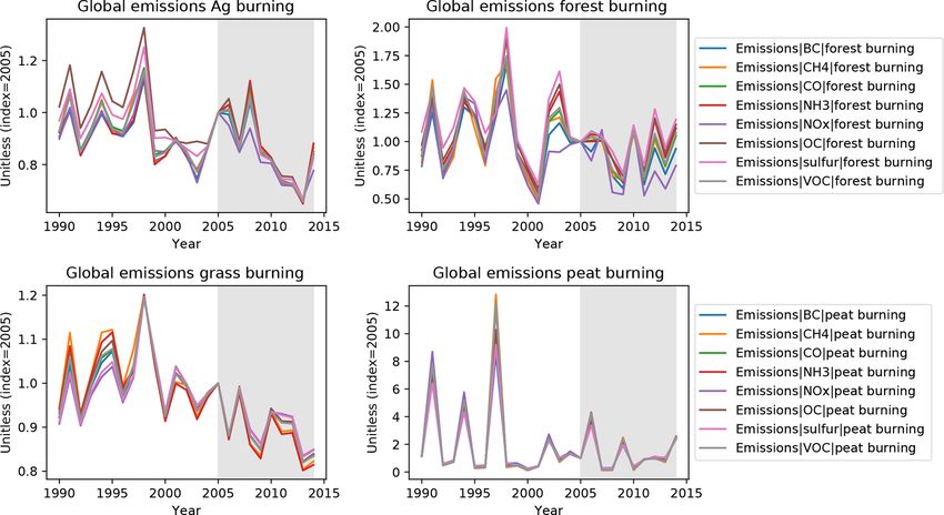
1446                                                        M. J. Gidden et al.: Global emissions pathways for use in CMIP6

whereas population increase is focused in low- and middle-         tal comparison to scenarios with high NTCFs for use in
income countries. Energy systems in SSP3 see a resurgence          AerChemMIP (Collins et al., 2017) contrasting with SSP3-
of coal dependence, whereas reductions occur in SSP4 as the        7.0 (see Appendix C for more detail on differences in as-
high-tech energy and economy sectors see increased devel-          sumptions between SSP3-7.0 and SSP3-LowNTCF). Both
opments and investments leading to higher diversification of       SSP4 scenarios fill gaps in Tier-1 forcing pathways and allow
technologies (Bauer et al., 2017). Policy making (either re-       investigations of impacts in scenarios with relatively strong
gionally or internally) in areas including land-use regulation,    land-use and aerosol climate effects but relatively low chal-
air pollution control, and GHG emissions limits is less effec-     lenges to mitigation. Finally, SSP5-3.4-OS allows for the
tive. Thus policies vary regionally in both SSPs with weak         study of a scenario in which there is large overshoot in RF
international institutions, resulting in the highest levels of     by mid-century followed by the implementation of substan-
pollutant and aerosol emissions and potential effect on cli-       tive policy tools to limit warming in the latter half of the cen-
mate outcomes (Shindell et al., 2013).                             tury. It is specifically designed to be twinned with SSP5-8.5,
   A matrix of socioeconomic–climate scenarios relevant to         following the same pathway through 2040, and support ex-
the broad scientific community was created with SSPs on one        periments examining delayed climate action.
axis and climate policy futures (i.e., mitigation scenarios) de-
lineated by end-of-century (EOC) RF on the other axis (see         2.2   Historical emissions data
Fig. 1). The scenarios selected for inclusion in ScenarioMIP,
shown in Table 1, are comprised of both baseline and mit-          We construct a common dataset of historical emissions for
igation cases, in which long-term climate policies are lack-       the year 20151 , the transition year in CMIP6 between his-
ing or included, respectively. They are divided into Tier-1        toric and future model runs, using two primary sources de-
scenarios, which span a wide range of uncertainty in future        veloped for CMIP6. Hoesly et al. (2018) provide data over
forcing and are utilized by other MIPs, and Tier-2 scenarios,      1750–2014 for anthropogenic emissions by country. They
which enable more detailed studies of the effect of mitigation     include a detailed sectoral representation (59 sectors in to-
and adaptation policies which fall between the Tier-1 forcing      tal) which has been aggregated into nine individual sectors
levels. Each scenario is run by a single model within Sce-         (see Appendix Table ), including agriculture, aircraft, en-
narioMIP, comprised of the AIM/CGE, GCAM4, IMAGE,                  ergy, industry, international shipping, residential and com-
MESSAGE-GLOBIOM, and REMIND-MAgPIE modeling                        mercial, solvent production and application, transportation,
teams. We provide a short discussion here on their selection       and waste. Values for 2015 were approximated by extend-
and refer the reader to O’Neill et al. (2016, Sect. 3.2.2) for     ing fossil fuel consumption using aggregate energy statistics
fuller discussion of the experimental design.                      (BP, 2016) and trends in emissions factors from the GAINS
   The Tier-1 scenarios include SSP1-2.6, SSP2-4.5, SSP3-          ECLIPSE V5a inventory (Klimont et al., 2017; Stohl et al.,
7.0, and SSP5-8.5, designed to provide a full range of forc-       2015). Sulfur (SOx ) emissions in China were trended from
ing targets similar in both magnitude and distribution to the      2010 using values from Zheng et al. (2018).
RCPs as used in CMIP5. Each EOC forcing level is paired               The study of van Marle et al. (2017) provides data on his-
with a specific SSP, which is chosen based on the relevant         torical emissions from open burning, specifically including
experimental coverage. For example, SSP2 is chosen for the         burning of agricultural waste on fields (AWB), forests, grass-
4.5 W m−2 experiment because of its high relevance as a ref-       lands, and peatlands out to 2015. Due to the high amount of
erence scenario to IAV communities as a scenario with in-          inter-annual variability in the historical data which is not ex-
termediate vulnerability and climate forcing and its median        plicitly modeled in IAMs, we use a decadal mean over 2005–
positioning of land use and aerosol emissions (of high impor-      2014 to construct a representative value for 2015 (see, e.g.,
tance for DAMIP and DCPP), whereas SSP3 is chosen for              Fig. A2). When used in conjunction with model results, we
the 7.0 W m−2 experiment as it allows for quantification of        aggregate country-level emissions to the individual model re-
avoided impacts (e.g., relative to SSP2) and has significant       gions of which they are comprised.
emissions from near-term climate forcing (NTCF) species               Emissions of N2 O and fluorinated gas species were har-
such as aerosols and methane (also referred to as short-lived      monized only at the global level, with 2015 values from
climate forcers, or SLCF).                                         other data sources. Global N2 O emissions were taken from
   The Tier-2 scenarios include SSP1-1.9, SSP3-LowNTCF,            PRIMAP (Gütschow et al., 2016) and global emissions of
SSP4-3.4, SSP4-6.0, and SSP5-3.4-Overshoot (OS), chosen            HFCs were developed by Velders et al. (2015). The HFC-
to both complement and extend the types of scenarios avail-        23 and total PFC and SF6 emissions were provided by Guus
able to climate modelers beyond those analyzed in CMIP5.           Velders, based on Carpenter et al. (2014) mixing ratios, and
SSP1-1.9 provides the lowest estimate of future forcing            were extended from 2012 to 2015 by using the average 2008–
matching the most ambitious goals of the Paris Agreement           2012 trend.
(i.e., “pursuing efforts to limit the [global average] temper-        1 For sulfur emissions in China, we include values up to 2017,
ature increase to 1.5 ◦ C above pre-industrial levels”). The       due to a drastic reduction in these emissions in the most recently
SSP3-LowNTCF scenario provides an important experimen-             available datasets.

Geosci. Model Dev., 12, 1443–1475, 2019                                              www.geosci-model-dev.net/12/1443/2019/
M. J. Gidden et al.: Global emissions pathways for use in CMIP6 1447
Table 1. All scenarios and associated attributes used in the ScenarioMIP experiment ensemble.
Target
forcing
Scenario level Scenario Contributing
name SSP (W m−2 ) type Tier IAM to other MIPs
SSP1-1.9 1 1.9 Mitigation 2 IMAGE ScenarioMIP
SSP1-2.6 1 2.6 Mitigation 1 IMAGE ScenarioMIP
SSP2-4.5 2 4.5 Mitigation 1 MESSAGE-GLOBIOM ScenarioMIP, VIACS AB, CORDEX,
GeoMIP, DAMIP, DCPP
SSP3-7.0 3 7 Baseline 1 AIM/CGE ScenarioMIP, AerChemMIP, LUMIP
SSP3-LowNTCF 3 6.3 Mitigation 2 AIM/CGE ScenarioMIP, AerChemMIP, LUMIP
SSP4-3.4 4 3.4 Mitigation 2 GCAM4 ScenarioMIP
SSP4-6.0 4 6 Mitigation 2 GCAM4 ScenarioMIP, GeoMIP
SSP5-3.4-OS 5 3.4 Mitigation 2 REMIND-MAGPIE ScenarioMIP
SSP5-8.5 5 8.5 Baseline 1 REMIND-MAGPIE ScenarioMIP, C4MIP, GeoMIP, ISMIP6, RFMIP
2.3 Automated emissions harmonization aircraft and international shipping sectors, and CO2 agricul-
ture, forestry, and other land-use (AFOLU) emissions due
Emissions harmonization is defined as a procedure designed to historical data availability and regional detail. Therefore
to match model results to a common set of historical emis- between 970 and 2776 emissions trajectories require harmo-
sions trajectories. The goal of this process is to match a spec- nization for any given scenario depending on the model used.
ified base-year dataset while retaining consistency with the We employ the newly available open-source software
original model results to the best extent possible while also Aneris (Gidden et al., 2018; Gidden, 2017) in order to per-
providing a smooth transition from historical trajectories. form harmonization in a consistent and rigorous manner. For
This non-disjoint transition is critical for global climate mod- each trajectory to be harmonized, Aneris chooses which har-
els when modeling projections of climate futures which de- monization method to use by analyzing both the relative dif-
pend on historical model runs, guaranteeing a smooth func- ference between model results and harmonization historical
tional shape of both emissions and concentration fields be- data as well as the behavior of the modeled emissions tra-
tween the historical and future runs. Models differ in their jectory. Available methods include ratio and offset methods,
2015 data points in part because the historical emissions which utilize the quotient and difference of unharmonized
datasets used to calibrate the models differ (e.g., PRIMAP – and harmonized values, respectively, as well as convergence
Gütschow et al., 2016; EDGAR – Crippa et al., 2016; CEDS methods, which converge to the original modeled results at
– Hoesly et al., 2018). Another cause of differences is that some future time period. We refer the reader to Gidden et al.
2015 is a projection year for all of these models (the original (2018) for a full description of the harmonization methodol-
scenarios were originally finalized in 2015). ogy and implementation.
Harmonization can be simple in cases where a model’s his- Override methods can be specified for any combination
torical data are similar to the harmonization dataset. How- of species, sectors, and regions which are used in place of
ever, when there are strong discrepancies between the two the default methods provided by Aneris. Override methods
datasets, the choice of harmonization method is crucial for are useful when default methods do not fully capture either
balancing the dual goals of accurate representation of model the regional or sectoral context of a given trajectory. Most
results and reasonable transitions from historical data to har- commonly, we observed this in cases where there are large
monized trajectories. relative differences in the historical datasets, the base-year
The quantity of trajectories requiring harmonization in- values are small, and there is substantial growth in the tra-
creases the complexity of the exercise. In this analysis, given jectory over the modeled time period, thereby reflecting the
the available sectoral representation of both the historical large relative difference in the harmonized emissions results.
data and models, we harmonize model results for 14 individ- However, the number of required override methods is small:
ual emissions species and 13 sectors as described in Table 2. 5.1 % of trajectories use override messages for the IMAGE
The majority of emissions–sector combinations are harmo- model, 5.6 % for MESSAGE-GLOBIOM, and 9.8 % for RE-
nized for every native model region2 (Table 3). Global tra- MIND. The AIM model elected not to use override methods,
jectories are harmonized for fluorinated species and N2 O, and GCAM uses a relatively large number (35 %).
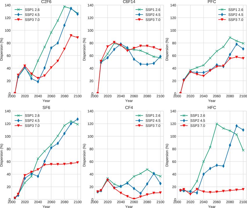
Finally, in order to provide additional detail for fluorinated
2 Further information regarding the model region definitions is
gases (F gases) we extend the set of reported HFC and CFC
available via the IAMC Wiki at https://www.iamcdocumentation.eu species based on exogenous scenarios. We take scenarios of
(last access: 8 April 2019) and Calvin et al. (2019).
www.geosci-model-dev.net/12/1443/2019/ Geosci. Model Dev., 12, 1443–1475, 2019
1448                                                                     M. J. Gidden et al.: Global emissions pathways for use in CMIP6

Table 2. Harmonized species and sectors, adapted from Gidden et al. (2018) with permission of the authors. A mapping of original model
variables (i.e., outputs) to ScenarioMIP sectors is shown in Appendix Table B2.

                                 Emissions species                                   Sectors
                                 Black carbon (BC)                                   Agricultural waste burningc
                                 Hexafluoroethane (C2 F6 )a                          Agriculturec
                                 Tetrafluoromethane (CF4 )a                          Aircraftb
                                 Methane (CH4 )                                      Energy sector
                                 Carbon dioxide (CO2 )c                              Forest burningc
                                 Carbon monoxide (CO)                                Grassland burningc
                                 Hydrofluorocarbons (HFCs)a                          Industrial sector
                                 Nitrous oxide (N2 O)a                               International shippingb
                                 Ammonia (NH3 )                                      Peat burningc
                                 Nitrogen oxides (NOx )                              Residential commercial other
                                 Organic carbon (OC)                                 Solvents production and application
                                 Sulfur hexafluoride (SF6 )a                         Transportation sector
                                 Sulfur oxides (SOx )                                Waste
                                 Volatile organic compounds (VOCs)
                               a Global total trajectories are harmonized due to lack of detailed historical data. b Global sectoral
                               trajectories are harmonized due to lack of detailed historical data. c A global trajectory for AFOLU
                               CO2 is used; non-land-use sectors are harmonized for each model region.

Table 3. The number of model regions and total harmonized emis-                       lated to fuel combustion and industrial and urban processes.
sions trajectories for each IAM participating in the study. The num-                  In order to preserve as much of the original model detail as
ber of trajectories is calculated from Table 2, including gas species                 possible, the downscaling procedures here begin with har-
for which global trajectories are harmonized.                                         monized emissions data at the level of native model regions
                                                                                      and the aggregate sectors (Table 2). Here we discuss key as-
                                                    Harmonized                        pects of the downscaling methodology and refer the reader
        Model                        Regions         trajectories                     to the downscaling documentation (https://github.com/iiasa/
        AIM/CGE                             17                1486                    emissions_downscaling/wiki, last access: 8 April 2019) for
        GCAM4                               32                2776                    further details.
        IMAGE                               26                2260                       AFOLU emissions, including agricultural waste burning,
        MESSAGE-GLOBIOM                     11                 970                    agriculture, forest burning, peat burning, and grassland burn-
        REMIND-MAGPIE                       11                 970                    ing, are downscaled using a linear method. Linear downscal-
                                                                                      ing means that the fraction of regional emissions in each
                                                                                      country stays constant over time. Therefore, the total amount
future HFCs from Velders et al. (2015), which provide de-                             of open-burning emissions allocated to each country will
tailed emissions trajectories for F gases. We downscale the                           vary over time as economies evolve into the future, follow-
global HFC emissions reported in each harmonized scenario                             ing regional trends from the native IAM. However there is
to arrive at harmonized emissions trajectories for all con-                           no subregional change in the spatial distribution of land-use
stituent F gases, deriving the HFC-23 from the RCP emis-                              related emissions over time. This is in contrast to other an-
sions pathway. We further include trajectories of CFCs as re-                         thropogenic emissions, where the impact, population, afflu-
ported in scenarios developed by the World Meteorological                             ence, and technology (IPAT) method is used to dynamically
Organization (WMO) (Carpenter et al., 2014), which are not                            downscale to the country level as discussed above. Note that
included in all model results.                                                        peat burning emissions were not modeled by the IAMs and
                                                                                      are constant into the future.
2.4    Region-to-country downscaling                                                     All other emissions are downscaled using the IPAT
                                                                                      (Ehrlich and Holdren, 1971) method developed by van Vu-
Downscaling, defined here as distributing aggregated re-                              uren et al. (2007), where population and GDP trajectories are
gional values to individual countries, is performed for all                           taken from the SSP scenario specifications (KC and Lutz,
scenarios in order to improve the spatial resolution of emis-                         2017; Dellink et al., 2015). The overall philosophy behind
sions trajectories, and as a prelude to mapping to a spatial                          this method is to assume that emissions intensity values (i.e.,
grid (discussed in Appendix D). We developed an automated                             the ratio of emissions to GDP) for countries within a region
downscaling routine that differentiates between two classes                           will converge from a base year, ti (2015 in this study), over
of sectoral emissions: those related to AFOLU and those re-

Geosci. Model Dev., 12, 1443–1475, 2019                                                                        www.geosci-model-dev.net/12/1443/2019/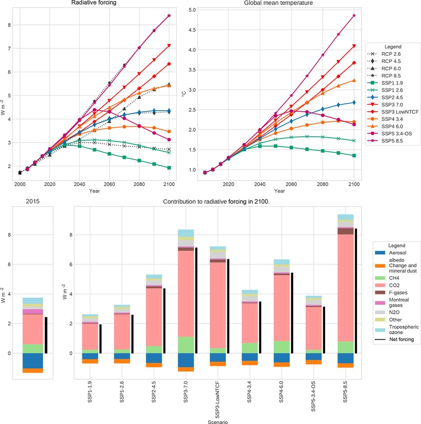
M. J. Gidden et al.: Global emissions pathways for use in CMIP6                                                             1449

the future. A convergence year, tf , is specified beyond 2100,    assume the development of substantial industrial activity in
the last year for the downscaled data, meaning that emissions     these countries.
intensities do not converge fully by 2100. The choice of con-        Finally, some scenarios include negative CO2 emissions
vergence year reflects the rate at which economic and energy      at some point in the future (notably from energy use). For
systems converge toward similar structures within each na-        CO2 emissions, therefore, we apply a linear rather than ex-
tive model region. Accordingly, the SSP1 and SSP5 scenarios       ponential function to allow a smooth transition to negative
are assigned relatively near-term convergence years of 2125,      emissions values for both the emissions intensity growth fac-
while SSP3 and SSP4 scenarios are assigned 2200, and SSP2         tor and future emissions intensity calculations. In such cases,
is assigned an intermediate value of 2150.                        Eqs. (2) and (3) are replaced by Eqs. (6) and (7), respectively.
   The downscaling method first calculates an emissions in-
tensity, I , for the base and convergence years using emissions              IR,tf        1
                                                                  βc =             −1                                         (6)
level, E, and GDP.                                                           Ic,ti     tf − ti
        Et
It =                                                       (1)
       GDPt
                                                                  Ic,t = (1 + βc )Ic,t−1                                      (7)
   An emissions intensity growth factor, β, is then deter-
mined for each country, “c”, within a model region, “R”, us-
ing convergence year emissions intensities, IR,tf , determined    3     Results
by extrapolating from the last 10 years (e.g., 2090 to 2100)
of the scenario data.                                             Here we present the results of harmonization and downscal-
                  1                                               ing applied to all nine scenarios under consideration. We dis-
       IR,tf   tf −ti
                                                                  cuss in Sect. 3.1 the relevance of each selected scenario to
βc =                                                       (2)
       Ic,ti                                                      the overall experimental design of ScenarioMIP, focusing on
                                                                  their RF and mean global temperature pathways. In Sect. 3.2,
   Using base-year data for each country and scenario data
                                                                  we discuss general trends in global trajectories of important
for each region, future downscaled emissions intensities and
                                                                  GHGs and aerosols and their sectoral contributions over the
patterns of emissions are then generated for each subsequent
                                                                  modeled time horizon. In Sect. 3.3, we explore the effect of
time period.
                                                                  harmonization on model results and the difference between
Ic,t = βc Ic,t−1                                           (3)    unharmonized and harmonized results. Finally, in Sect. 3.4,
                                                                  we provide an overview of the spatial distribution of emis-
                                                                  sions species at both regional and spatial grids.
 ∗
Ec,t = Ic,t GDPc,t                                         (4)    3.1    Experimental design and global climate response
   These spatial patterns are then scaled with (i.e., normal-
                                                                  The nine ScenarioMIP scenarios were selected to provide a
ized to) the model region data to guarantee consistency be-
                                                                  robust experimental design space for future climate studies
tween the spatial resolutions, resulting in downscaled emis-
                                                                  as well as IAV analyses with the broader context of CMIP6.
sions for each country in each time period.
                                                                  Chief among the concerns in developing such a design space
                ER,t     ∗                                        are both the range and spacing of the global climate re-
Ec,t = P             ∗ Ec,t                                (5)    sponse within the portfolio of scenarios (Moss et al., 2008).
                0  E  0
               c ∈R c ,t
                                                                  Prior work for the RCPs studied a range of climate out-
   For certain countries and sectors the historical dataset has   comes between ∼ 2.6 and 8.5 W m−2 at EOC. Furthermore,
zero-valued emissions in the harmonization year. This would       recent work (Tebaldi et al., 2015) finds that statistically sig-
result in zero downscaled future emissions for all years. Zero    nificant regional temperature outcomes (> 5 % of half the
emissions data occur largely for small countries, many of         land surface area) are observable with a minimum separation
them small island nations. This could be due to either lack       of 0.3 ◦ C, which is approximately equivalent to 0.75 W m−2
of actual activity in the base year or missing data on activ-     (O’Neill et al., 2016). Given the current policy context, no-
ity in those countries. In order to allow for future sectoral     tably the recent adoption of the UN Paris Agreement, the pri-
growth in such cases, we adopt, for purposes of the above         mary design goal for the ScenarioMIP scenario selection is
calculations, an initial emissions intensity of one-third the     thus twofold: span a wider range of possible climate futures
value of the lowest country in the same model region. We          (1.9–8.5 W m−2 ) in order to increase relevance to the global
then allocate future emissions in the same manner discussed       climate dialogue and provide a variety of scenarios between
above, which is consistent with our overall convergence as-       these upper and lower bounds such that they represent sta-
sumptions. Note that we exclude the industrial sector (Ta-        tistically significant climate variations in order to support a
ble 2) from this operation as it might not be reasonable to       wide variety of CMIP6 analyses.

www.geosci-model-dev.net/12/1443/2019/                                                 Geosci. Model Dev., 12, 1443–1475, 2019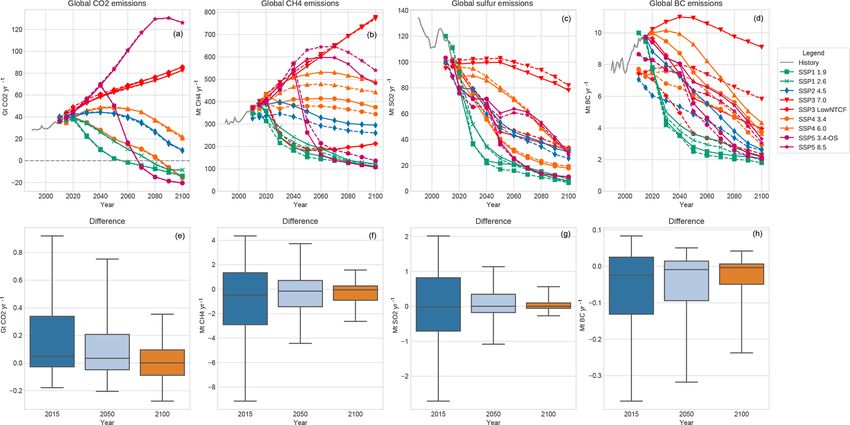
1450                                                       M. J. Gidden et al.: Global emissions pathways for use in CMIP6

   We find that the selected scenarios meet this broad goal,      scenario. SSP3-LowNTCF sees substantially fewer contribu-
as shown in Fig. 2, by using the simple climate model MAG-        tions to EOC forcing from NTCF emissions (notably SOx
ICC6 with central climate-system and gas-cycle parameter          and methane), resulting in a forcing level of 6.3 W m−2 and
settings for all scenarios to calculate pathways of both RF       global mean temperature increase of 3.75 ◦ C by the end of
and the resulting response of global mean temperature (see        the century. This significant reduction is largely due to updat-
Appendix Table B3 for a listing of all EOC RF values).            ing emissions coefficients for air pollutants and other NTCFs
   We also present illustrative global mean temperature path-     to match the SSP1 assumptions. SSP4-3.4 was chosen to pro-
ways. EOC temperature outcomes span a large range, from           vide a scenario at the lower end of the range of future forc-
1.4 ◦ C at the lower end to 4.9 ◦ C for SSP5-8.5, the scenario    ing pathways. Reaching a EOC mean global temperature be-
with the highest warming emissions trajectories. Notably,         tween SSP2-4.5 and SSP1-2.6 (∼ 2.25 ◦ C), it is an ideal sce-
two scenarios (SSP1-1.9, which reaches 1.4 ◦ C by EOC, and        nario for scientists to study the mitigation costs and associ-
SSP1-2.6, reaching 1.7 ◦ C) can be used for studies of global     ated impacts between forcing levels of 4.5 and 2.6 W m−2 .
outcomes of the implementation of the UN Paris Agreement,            The final two scenarios, SSP1-1.9 and SSP5-3.4-OS,
which has a desired goal of “[h]olding the increase in the        were chosen to study policy-relevant questions of near- and
global average temperature to well below 2 ◦ C above pre-         medium-term action on climate change. SSP1-1.9 provides
industrial levels and pursuing efforts to limit the temperature   a new low end to the RF pathway range. It reaches an EOC
increase to 1.5 ◦ C above pre-industrial levels” (United Na-      forcing level of ∼ 1.9 W m−2 and an associated global mean
tions, 2016, Article 2.1(a)). The difference between scenario     temperature increase of ∼ 1.4 ◦ C (with temperature peaking
temperature outcomes is statistically significant in nearly       in 2040), in line with the goals of the Paris Agreement. SSP5-
all cases, with a minimum difference of 0.37 ◦ C (SSP1-1.9        3.4-OS, however, is designed to represent a world in which
and SSP1-2.6) and maximum value of 0.77 ◦ C (SSP3-7.0             action towards climate change mitigation is delayed but vig-
and SSP5-8.5). The EOC difference between SSP4-3.4 and            orously pursued after 2050, resulting in a forcing and mean
SSP5-3.4-OS is not significant (0.07 ◦ C); however global cli-    global temperature overshoot. A peak temperature of 2.5 ◦ C
mate outcomes are likely sensitive to the dynamics of the         above pre-industrial levels is reached in 2060 after which
forcing pathway (Tebaldi et al., 2015).                           global mitigation efforts reduce EOC warming to ∼ 2.25 ◦ C.
   A subset of four scenarios (SSP1-2.6, SSP2-4.5, SSP4-6.0,      In tandem, and including SSP2-4.5 (which serves as a refer-
and SSP5-8.5) was also designed to provide continuity be-         ence experiment in ScenarioMIP; O’Neill et al., 2016), these
tween CMIP5 and CMIP6 by providing similar forcing path-          scenarios provide a robust experimental platform to study the
ways to their RCP counterparts assessed in CMIP5. We find         effect of the timing and magnitude of global mitigation ef-
that this aspect of the scenario design space is also met by      forts, which can be especially relevant to science-informed
the relevant scenarios. SSP2-4.5 and SSP5-8.5 track RCP4.5        policy discussions.
and RCP8.5 pathways nearly exactly. We observe slight de-
viations between SSP1-2.6 and RCP2.6 as well as SSP4-6.0          3.2   Global emissions trajectories
and RCP6.0 at mid-century due largely to increased methane
emissions in the historic period (i.e., methane emissions         Emissions contributions to the global climate system are
broadly follow RCP8.5 trajectories after 2000, resulting in       myriad but can broadly be divided into contributions from
higher emissions in the harmonization year of this exercise;      greenhouse gases (GHGs) and aerosols. The models used in
see Fig. 3 below).                                                this analysis explicitly represent manifold drivers and pro-
   The remaining five scenarios were chosen to “fill gaps” in     cesses involved in the emissions of various gas species. For
the previous RCP studies in CMIP5 and enhance the poten-          a fuller description of these scenario results see the orig-
tial policy relevance of CMIP6 MIP outputs (O’Neill et al.,       inal SSP quantification papers (van Vuuren et al., 2017;
2016). SSP3-7.0 was chosen to provide a scenario with rel-        Fricko et al., 2017; Fujimori et al., 2017; Calvin et al.,
atively high vulnerability and land-use change with associ-       2017; Kriegler et al., 2017). Here, we focus on emissions
ated near-term climate forcing (NTCF) emissions resulting         species that most strongly contribute to changes in future
in a high RF pathway. We find that it reaches an EOC forc-        mean global temperature and scenarios with the highest rele-
ing target of ∼ 7.1 W m−2 and greater than 4 ◦ C mean global      vance and uptake for other MIPs within CMIP6, namely the
temperature increase. While contributions to RF from CO2          Tier-1 scenarios SSP1-2.6, SSP2-4.5, SSP3-7.0, and SSP5-
in SSP3-7.0 are lower than that of SSP5-8.5, methane and          8.5. Where insightful, we provide additional detail on results
aerosol contributions are considerably higher (see, e.g., Et-     from other scenarios; however results for all scenarios are
minan et al., 2016, for a discussion on the effect of shortwave   available in Appendix E.
forcing on methane’s contribution to overall RF). A compan-          CO2 emissions have a large span across scenarios by the
ion scenario, SSP3-LowNTCF, was also included in order to         end of the century (−20 to 125 Gt yr−1 ), as shown in Fig. 3.
study the effect of NTCF species in the context of AerChem-       Scenarios can be categorized based on characteristics of their
MIP. Critically, emissions factors of key NTCF species are        trajectory profiles: those that have consistent downward tra-
assumed to develop similar to an SSP1 (rather than SSP3)          jectories (SSP1, SSP4-3.4), those that peak in a given year

Geosci. Model Dev., 12, 1443–1475, 2019                                             www.geosci-model-dev.net/12/1443/2019/
M. J. Gidden et al.: Global emissions pathways for use in CMIP6                                                                    1451

Figure 2. Trajectories of RF and global mean temperature (above pre-industrial levels) are presented as are the contributions to RF for a
number of different emissions types native to the MAGICC6 model. The RF trajectories are displayed with their RCP counterparts analyzed
in CMIP5. For those scenarios with direct analogues, trajectories are largely similar in shape and match the same EOC forcing values.

and then decrease in magnitude (SSP2-4.5 in 2040 and SSP4-             cross the zero-emissions threshold in 2070, 2080, and 2090,
6.0 in 2050), and those that have consistent growth in emis-           respectively.
sions (SSP3). SSP5 scenarios, which model a world with                    Global emissions trajectories for CO2 are driven largely by
fossil-fuel-driven development, have EOC emissions which               the behavior of the energy sector in each scenario, as shown
bound the entire scenario set, with the highest CO2 emissions          in Fig. 4. Positive emissions profiles are also greatly influ-
in SSP5-8.5 peaking in 2080 and the lowest CO2 emissions               enced by the industry and transport sectors, whereas negative
in SSP5-3.4-OS resulting from the application of stringent             emissions profiles are driven by patterns of agriculture and
mitigation policies after 2040 in an attempt to stabilize RF           land-use as well as the means of energy production. In SSP1-
to 3.4 W m−2 after overshooting this limit earlier in the cen-         2.6, early to mid-century emissions continue to be dominated
tury. A number of scenarios exhibit negative net CO2 emis-             by the energy sector with substantial contributions from in-
sions before the end of the century. SSP1-1.9, the scenario            dustry and transport. Negative emissions from land use are
with the most consistent negative emissions trajectory, first          observed as early as 2030 due to large-scale afforestation
reports net negative emissions in 2060 with EOC emissions              (Popp et al., 2017; van Vuuren et al., 2017) while net neg-
of −14 Gt yr−1 . SSP5-3.4-OS, SSP1-2.6, and SSP4-3.4 each              ative emissions from energy conversion first occur in 2070.
                                                                       Such net negative emissions are achieved when carbon diox-

www.geosci-model-dev.net/12/1443/2019/                                                    Geosci. Model Dev., 12, 1443–1475, 2019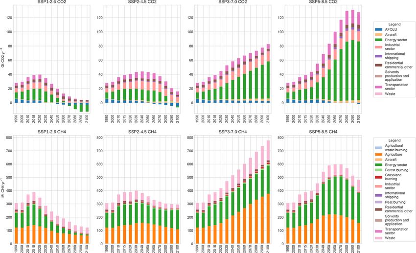
1452                                                          M. J. Gidden et al.: Global emissions pathways for use in CMIP6

Figure 3. Trajectories of CO2 and CH4 , primary contributors to GHG emissions, including both historical emissions, emissions analyzed for
the RCPs, and all nine scenarios covered in this study.

ide removal from bioenergy from carbon capture and storage             jectories to CO2 , with large emissions reductions; SSP2 fol-
(CCS) exceeds residual fossil CO2 emissions from the com-              lows suit, with emissions peaking in 2030 and then reduc-
bustion of coal, oil, and gas. Emissions contributions from            ing throughout the rest of the century; in SSP3’s baseline
the transport sector diminish over the century as heavy- and           scenario, emissions continue to grow while in the NTCF
light-duty transport fleets are electrified. Emissions from in-        scenario they are reduced drastically as policies are imple-
dustry peak and the decrease over time such that the resi-             mented to reduce forcing from short-lived emissions species;
dential and commercial sector (RC) provides the majority of            SSP4 is characterized by growing (SSP4-6.0) or mostly sta-
positive CO2 emissions by the end of the century. SSP2-4.5             ble (SSP4-3.4) CH4 emissions until the middle of the cen-
experiences similar trends among sectors but with smaller              tury which peak in 2060 and then decline; and finally SSP5’s
magnitudinal changes and temporal delays. Negative emis-               baseline scenario sees a plateauing of CH4 emissions be-
sions, for example, are experienced in the land-use sector for         tween 2050 and 2070 before their eventual decline, while the
the first time in 2060 and are not experienced in the energy           overshoot scenario has drastic CH4 emissions reductions in
sector until the end of the century. Energy-sector CO2 emis-           2040 corresponding to significant mid-century mitigation ef-
sions continue to play a large role in the overall composition         forts in that scenario.
until 2080, at which point the industrial sector provides the             Historically, CH4 emissions are dominated by three sec-
plurality of CO2 . Emissions from the transport sector peak at         tors: energy (due to fossil fuel production and natural gas
mid-century, but are still a substantive component of positive         transmission), agriculture (largely enteric fermentation from
CO2 emissions at the end of the century. Finally, the SSP5-            livestock and rice production), and waste (i.e., landfills). In
8.5 scenario’s emissions profile is dominated by the fossil-           each scenario, global emissions of CH4 are largely domi-
fueled energy sector for the entirety of the century. Contribu-        nated by the behavior of activity in each of these sectors
tions from the transport and industrial sectors grow in magni-         over time. For example, in the SSP1 scenarios, significant re-
tude but are diminished as the share of total CO2 emissions,           ductions in energy emissions are observed as energy supply
CO2 emissions from the AFOLU sector, decrease steadily                 systems shift from fossil to renewable sources while agri-
over time. By the end of the century, the energy sector com-           culture and waste-sector emissions see only modest reduc-
prises almost 75 % of all emitted CO2 in this scenario relative        tions as global population stabilizes around mid-century. In
to 50 % today.                                                         the SSP2 scenario, emissions from the energy sector peak in
   Methane (CH4 ) is an emissions species with substantial             2040 as there is continued reliance on energy from natural
contributions to potential future warming mainly due to its            gas but large expansions in renewables in the future; how-
immediate GHG effect, but also because of its influence on             ever, emissions from the agricultural and waste sectors are
atmospheric chemistry, as a tropospheric ozone precursor,              similar to today’s levels by the end of the century. Finally,
and its eventual oxidation into CO2 in the case of CH4 from            CH4 emissions in SSP5’s baseline scenario are characterized
fossil sources (Boucher et al., 2009). At present, approxi-            by growth in the energy sector from continued expansion of
mately 400 Mt yr−1 of CH4 is emitted globally, and the span            natural gas and a peak and reduction in agricultural emissions
of future emissions developed in this scenario set range from          resulting in 20 % higher emissions at the end of the century
100 to nearly 800 Mt yr−1 by the end of the century. Global            relative to the present as population grows in the near term
emissions of methane in SSP1 scenarios follow similar tra-             before contracting globally.

Geosci. Model Dev., 12, 1443–1475, 2019                                                   www.geosci-model-dev.net/12/1443/2019/
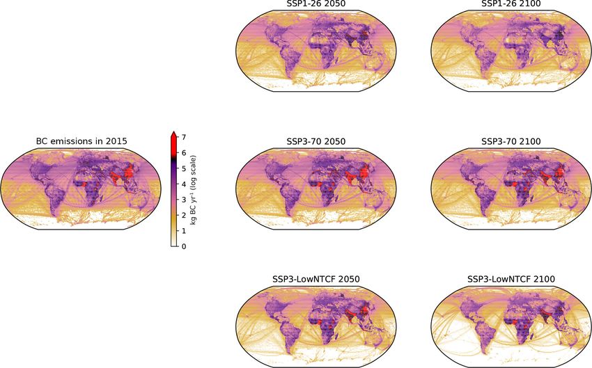
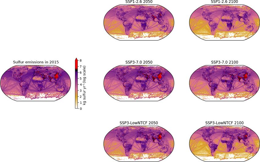
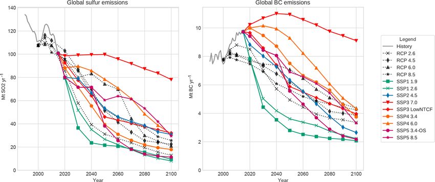
M. J. Gidden et al.: Global emissions pathways for use in CMIP6                                                                   1453

Figure 4. The sectoral contributions to CO2 and CH4 emissions for Tier-1 scenarios.

   GHG emissions are broadly similar between the main                  sector transitions to non-fossil-based fuels and end-of-pipe
scenarios in CMIP5 (RCPs) and CMIP6 (SSPs). Notably,                   measures for air pollution control are ramped up swiftly. The
we observe that the SSPs exhibit slightly lower CO2 emis-              residual amount of sulfur remaining at the end of the century
sions in the 2.6 W m−2 scenarios and higher emissions in the           (∼ 10 Mt yr−1 ) is dominated by the industrial sector. SSP2-
8.5 W m−2 scenarios due to lower and higher dependence on              4.5 sees a similar transition but with delayed action: total sul-
fossil fuels relative to their RCP predecessors. CH4 emis-             fur emissions decline due primarily to the decarbonization of
sions are largely similar at EOC for 2.6 and 4.5 W m−2 sce-            the energy sector. SSP5 also observes declines in overall sul-
narios between the RCPs and SSPs, with earlier values dif-             fur emissions led largely by an energy mix that transitions
fering due to continued growth in the historical period (RCPs          from coal dependence to dependence on natural gas, as well
begin in 2000 whereas SSPs begin in 2015). The 8.5 W m−2               as strong end-of-pipe air pollution control efforts. These re-
scenario exhibits the largest difference in CH4 emissions be-          ductions are similarly matched in the industrial sector, where
tween the RCPs and SSPs because of the SSP5 socioeco-                  natural gas is substituted for coal use as well. Thus, overall
nomic story line depicting a world which largely develops              reductions in emissions are realized across the scenario set.
out of poverty in less-developed countries, reducing CH4               Only SSP3 shows EOC sulfur emissions equivalent to the
emissions from waste and agriculture. This contrasts with a            present day, largely due to increased demand for industrial
very different story line behind RCP8.5 (Riahi et al., 2011).          services from growing population centers in developing na-
   In nearly all scenarios, aerosol emissions are observed to          tions with a heavy reliance on coal-based energy production
decline over the century; however, the magnitude and speed             and weak air pollution control efforts.
of this decline are highly dependent on the evolution of vari-            Aerosols associated with the burning of traditional
ous drivers based on the underlying SSP story lines, resulting         biomass, crop, and pasture residues, as well as municipal
in a wide range of aerosol emissions, as shown in Fig. 5.              waste, such as black carbon (BC) and organic carbon (OC,
For example, sulfur emissions (totaling 112 Mt yr−1 glob-              see Appendix Fig. E3), are affected most strongly by the de-
ally in 2015) are dominated at present by the energy and in-           gree of economic progress and growth in each scenario, as
dustrial sectors. In SSP1, where the world transitions away            shown in Fig. 6. For example, BC emissions from the res-
from fossil-fuel-related energy production (namely coal in             idential and commercial sector comprise nearly 40 % of all
the case of sulfur), emissions decline sharply as the energy           emissions in the historical time period with a significant con-

www.geosci-model-dev.net/12/1443/2019/                                                   Geosci. Model Dev., 12, 1443–1475, 2019
1454                                                           M. J. Gidden et al.: Global emissions pathways for use in CMIP6

Figure 5. Emissions trajectories for sulfur and black carbon (BC), for history, the RCPs, and all nine scenarios analyzed in this study. SSP
trajectories largely track with RCP values studied in CMIP5. A notable difference lies in BC emissions, which have seen relatively large
increases in past years, thus providing higher initial emissions for the SSPs.

tribution from mobile sources. By the end of the century,               atively closely to the magnitude of model results due to gen-
however, emissions associated with crop and pasture activ-              eral agreement between historical sources used by individual
ity comprise the plurality of total emissions in SSP1, SSP2,            models and the updated historical emissions datasets. This
and SSP5 due to a transition away from traditional biomass              leads to convergence harmonization routines being used by
usage based on increased economic development and popu-                 default. In the case of CH4 and BC, however, there is larger
lation stabilization and emissions controls on mobile sources.          disagreement between model results and harmonized results
Only SSP3, in which there is continued global inequality                in the base year. In such cases, Aneris chooses harmonization
and the persistence of poor and vulnerable urban and rural              methods that match the shape of a given trajectory rather than
populations, are there continued quantities of BC emissions             its magnitude in order to preserve the relationship between
across sectors similar to today. OC emissions are largely               driver and emissions for each model.
from biofuel and open burning and follow similar trends:                   We find that across all harmonized trajectories the differ-
large reductions in scenarios with higher income growth rates           ence between harmonized and unharmonized model results
with a residual emissions profile due largely to open-burning-          decreases over the modeled time horizon. Panels (e–h) in
related emissions. Other pollutant emissions (e.g., NOx , car-          Fig. 7 show the distribution of all 15 954 trajectories (unhar-
bon monoxide, CO; and volatile organic carbon, VOC) also                monized and less harmonized result) for the harmonization
see a decline in total global emissions at rates depending on           year (2015) and two modeled years (2050 and 2100). Each
the story line (Rao et al., 2017).                                      emissions species data population exhibits the same trend of
                                                                        reduced difference between modeled and harmonized results.
3.3    The effects of harmonization                                     Not only does the deviation of result distributions decrease
                                                                        over time, but the median value also converges toward zero
                                                                        in all cases.
Harmonization, by definition, modifies the original model
                                                                           The trajectory behavior for a number of important emis-
results such that base-year values correspond to an agreed-
                                                                        sions species is dominated by certain sectors, as shown in
upon historical source, with an aim for future values to match
                                                                        Appendix Fig. F1. Notably, the energy sector tends to domi-
the original model behavior as much as possible. Model re-
                                                                        nate behavior of CO2 emissions, agriculture dominates CH4
sults are harmonized separately for each individual combi-
                                                                        emissions trajectories, the industrial sector largely deter-
nation of model region, sector, and emissions species. In the
                                                                        mines total sulfur emissions, and emissions from the resi-
majority of cases, model results are harmonized using the de-
                                                                        dential and commercial sectors tend to dominate BC emis-
fault methods described in Sect. 2.3; however, it is possible
                                                                        sions across the various scenarios. Accordingly, we further
for models to provide harmonization overrides in order to ex-
                                                                        analyzed the harmonization behavior of these sector–species
plicitly set a harmonization method for a given trajectory.
                                                                        combinations. Importantly, we again observe an overall trend
   We assess the impact that harmonization has on model re-
                                                                        towards convergence of results at the end of the century;
sults by analyzing the harmonized and unharmonized tra-
                                                                        thus harmonized results largely track unharmonized results
jectories. Figure 7 shows global trajectories for each sce-
                                                                        for these critical emissions sectors. The deviation of distri-
nario of a selected number of emissions species. Qualita-
                                                                        butions of differences consistently decreases with time for
tively, the CO2 and sulfur emissions trajectories match rel-

Geosci. Model Dev., 12, 1443–1475, 2019                                                    www.geosci-model-dev.net/12/1443/2019/
M. J. Gidden et al.: Global emissions pathways for use in CMIP6 1455 Figure 6. The sectoral contributions to sulfur and black carbon emissions for Tier-1 scenarios. Figure 7. Harmonized (solid) and unharmonized (dashed) trajectories are shown are shown in Panels (a)–(d). Panels (e)–(h) depict the distribution of differences (harmonized and less unharmonized) for every modeled region. All box plots show upper and lower quartiles as solid boxes, median values as solid lines, and whiskers extending to the 10th and 90th percentiles. Median values for all are near zero; however, the deviation decreases with time as harmonized values begin to more closely match unharmonized model results largely due to the use of convergence methods. www.geosci-model-dev.net/12/1443/2019/ Geosci. Model Dev., 12, 1443–1475, 2019
1456                                                      M. J. Gidden et al.: Global emissions pathways for use in CMIP6

all scenarios, and nearly all medians converge consistently      as local and regional air quality. Thus in order to provide cli-
towards zero, save for energy-related CO2 SSP5-8.5, which        mate models with more detailed and meaningful datasets, we
has a higher growth rate than convergence rate, thus larger      downscale emissions trajectories from model regions to indi-
differences in 2050 than 2015. Overall, we find the harmo-       vidual countries. In most cases, models explicitly represent
nization procedure successfully harmonized results’ histori-     countries with large shares of emissions (e.g., USA, China,
cal base year and closely matches model results across the       India). MESSAGE-GLOBIOM and REMIND-MAGPIE are
scenarios by EOC.                                                notable exceptions; however, their regional aggregations are
                                                                 such that these important countries comprise the bulk of
3.4    Spatial distribution of emissions                         emissions in their aggregate regions (e.g., the MESSAGE-
                                                                 GLOBIOM North American region comprises the USA and
The extent to which reductions or growth of emissions are        Canada). For regions constituted by many countries, country-
distributed regionally varies greatly among scenarios. The re-   level emissions are driven largely by bulk region emissions
gional breakdown of primary contributors to future warming       and country GDP in each scenario (per Sect. 2.4). After-
potential, CO2 and CH4 , is shown in Fig. 8. While present-      wards, country-level emissions are subsequently mapped to
day CO2 emissions see near-equal contributions from the          spatial grids (Feng, 2019). We here present global maps of
Organization for Economic Cooperation and Development            two aerosol species with the strongest implications on future
(OECD) and Asia, future CO2 emissions are governed               warming, i.e., BC in Fig. 9 and sulfur in Fig. 10. We high-
largely by potential developments in Asia (namely China          light three cases which have relevant aerosol emissions pro-
and India). For SSP1-2.6, in which deep decarbonization and      files: SSP1-2.6, which has significantly decreasing emissions
negative CO2 emissions occur before the end of the cen-          over the century, SSP3-7.0, which has the highest aerosol
tury, emissions in Asia peak in 2020 before reducing to zero     emissions, and SSP3-LowNTCF, which has socioeconomic
by 2080. Mitigation efforts occur across all regions, and the    drivers similar to those of the SSP3 baseline but models the
majority of carbon reduction is focused in the OECD; how-        inclusion of policies which seek to limit emissions of near-
ever, all regions have net negative CO2 emissions by 2090.       term climate forcing species.
Asian CO2 emissions in SSP2-4.5 peak in 2030, and most              At present, BC has the highest emissions in China and In-
other regions see overall reductions except Africa, in which     dia due largely to traditional biomass usage in the residential
continued development and industrialization results in emis-     sector and secondarily to transport-related activity. In sce-
sions growth. Notably, Latin America is the only region in       narios of high socioeconomic development and technologi-
which negative emissions occur in SSP2-4.5 due largely to        cal progress, such as SSP1-2.6, emissions across countries
increased deployment of biomass-based energy production          decline dramatically such that by the end of the century, to-
and carbon sequestration. Sustained growth across regions        tal emissions in China, for example, are equal to those of
is observed in SSP5-8.5, where emissions in Asia peak by         the USA today. In almost all countries, BC emissions are
2080, driving the global emissions peaking in the same year.     nearly eradicated by mid-century while emissions in south-
Other scenarios (see Appendix Fig. G1) follow similar trends     east Asia reach similar levels by the end of the century. In
with future CO2 emissions driven primarily by developments       SSP3-7.0, however, emissions from southeast Asia and cen-
in Asia.                                                         tral Africa increase until the middle of the century as pop-
   CH4 emissions, resulting from a mix of energy use, food       ulations grow while still depending on fossil-fuel-heavy en-
production, and waste disposal, show a different regional        ergy supply technologies, transportation, and cooking fuels.
breakdown across scenarios. In SSP1-2.6, CH4 emissions are       By the end of the century in SSP3-7.0, global BC emissions
reduced consistently across regions as energy systems tran-      are nearly equivalent to the present day (see, e.g., Fig. 5), but
sition away from fossil fuel use (notably natural gas) and the   these emissions are concentrated largely in central Africa,
husbandry of livestock is curtailed globally. CH4 emissions      southeast Asia, and Brazil while they are reduced in North
in other scenarios tend to be dominated by developments in       America, Europe, and central Asia. By enacting policies
Africa. In SSP5-8.5, for example, emissions in Africa begin      that specifically target near-term climate forcers in SSP3-
to dominate the global profile by mid-century, due largely to    LowNTCF, the growth of emissions in the developing world
expansion of fossil-fuel-based energy production. SSP3 and       is muted by mid-century and is cut by more than half of
SSP4 see continued growth in African CH4 emissions across        today’s levels (∼ 9 vs. ∼ 4 Mt yr−1 ) by the end of the cen-
the century, even when global emissions are reduced as in the    tury. These policies result in similar levels of BC emissions
case of SSP4 scenarios.                                          in China as in SSP1-2.6, while most of the additional emis-
   CO2 and CH4 are well-mixed climate forcers (Stocker           sions are driven by activity in India and central Africa due
et al., 2013) and thus their spatial variation has a higher      to continued dependence on traditional biomass for cooking
impact from a political rather than physical perspective.        and heating.
Aerosols, however, have substantive spatial variability which       The spatial distribution of sulfur emissions varies from
directly impacts both regional climate forcing via scattering    that of BC due to large contributions from energy and in-
and absorption of solar radiation and cloud formation as well    dustrial sectors, and is thus being driven by a country’s eco-

Geosci. Model Dev., 12, 1443–1475, 2019                                            www.geosci-model-dev.net/12/1443/2019/
You can also read