Exploring mechanisms responsible for tidal modulation in flow of the Filchner-Ronne Ice Shelf
←
→
Page content transcription
If your browser does not render page correctly, please read the page content below
The Cryosphere, 14, 17–37, 2020
https://doi.org/10.5194/tc-14-17-2020
© Author(s) 2020. This work is distributed under
the Creative Commons Attribution 4.0 License.

Exploring mechanisms responsible for tidal modulation in flow of
the Filchner–Ronne Ice Shelf
Sebastian H. R. Rosier and G. Hilmar Gudmundsson
Department of Geography and Environmental Sciences, Northumbria University, Newcastle upon Tyne, NE1 8ST, UK

Correspondence: Sebastian H. R. Rosier (sebastian.rosier@northumbria.ac.uk)

Received: 18 April 2019 – Discussion started: 7 May 2019
Revised: 28 November 2019 – Accepted: 30 November 2019 – Published: 9 January 2020

Abstract. An extensive network of GPS sites on the                  zontal short-period semidiurnal tidal motion, causing twice-
Filchner–Ronne Ice Shelf and adjoining ice streams shows            daily flow reversals at the ice front, can be generated through
strong tidal modulation of horizontal ice flow at a range of        a purely elastic response to basin-wide tidal perturbations
frequencies. A particularly strong (horizontal) response is         in the ice shelf slope. This model also allows us to quan-
found at the fortnightly (Msf ) frequency. Since this tidal con-    tify the effect of tides on mean ice flow and we find that the
stituent is absent in the (vertical) tidal forcing, this observa-   Filchner–Ronne Ice Shelf flows, on average, ∼ 21 % faster
tion implies the action of some non-linear mechanism. An-           than it would in the absence of large ocean tides.
other striking aspect is the strong amplitude of the flow per-
turbation, causing a periodic reversal in the direction of ice
shelf flow in some areas and a 10 %–20 % change in speed at
grounding lines. No model has yet been able to reproduce the        1   Introduction
quantitative aspects of the observed tidal modulation across
the entire Filchner–Ronne Ice Shelf. The cause of the tidal         Much of the Antarctic Ice Sheet is surrounded by floating ice
ice flow response has, therefore, remained an enigma, indi-         shelves, and early research suggested that these ice shelves
cating a serious limitation in our current understanding of the     may have a significant mechanical impact on upstream flow
mechanics of large-scale ice flow. A further limitation of pre-     (Thomas, 1973; Hughes, 1973). More recently, observations
vious studies is that they have all focused on isolated regions     following ice shelf disintegration and modelling efforts have
and interactions between different areas have, therefore, not       confirmed this “buttressing” effect and enabled a quantifi-
been fully accounted for. Here, we conduct the first large-         cation of its importance (Rott et al., 2002; De Angelis and
scale ice flow modelling study to explore these processes us-       Skvarca, 2003; Rignot et al., 2004; Furst et al., 2018; Reese
ing a viscoelastic rheology and realistic geometry of the en-       et al., 2018). Ice shelves are now thought to modify upstream
tire Filchner–Ronne Ice Shelf, where the best observations of       flow and to impact the stability regime of grounding lines
tidal response are available. We evaluate all relevant mech-        (Gudmundsson, 2013; Pegler, 2018; Haseloff and Sergienko,
anisms that have hitherto been put forward to explain how           2018). Understanding the mechanics of ice shelf flow is,
tides might affect ice shelf flow and compare our results with      therefore, of considerable importance for assessing the fu-
observational data. We conclude that, while some are able to        ture evolution of ice discharge from the ice sheet’s interior,
generate the correct general qualitative aspects of the tidally     across grounding lines and into the ocean.
induced perturbations in ice flow, most of these mechanisms            Recently, an increasing quantity of GPS and InSAR ob-
must be ruled out as being the primary cause of the observed        servations have revealed that the flow of both ice shelves
long-period response. We find that only tidally induced lat-        and ice streams can be strongly modulated by ocean tides,
eral migration of grounding lines can generate a sufficiently       leading to substantial temporal variations in velocity (Riedel
strong long-period Msf response on the ice shelf to match           et al., 1999; Doake et al., 2002; Legresy et al., 2004; Brunt
observations. Furthermore, we show that the observed hori-          et al., 2010; King et al., 2011; Alley, 1997; Bindschadler
                                                                    et al., 2003; Anandakrishnan et al., 2003; Gudmundsson,

Published by Copernicus Publications on behalf of the European Geosciences Union.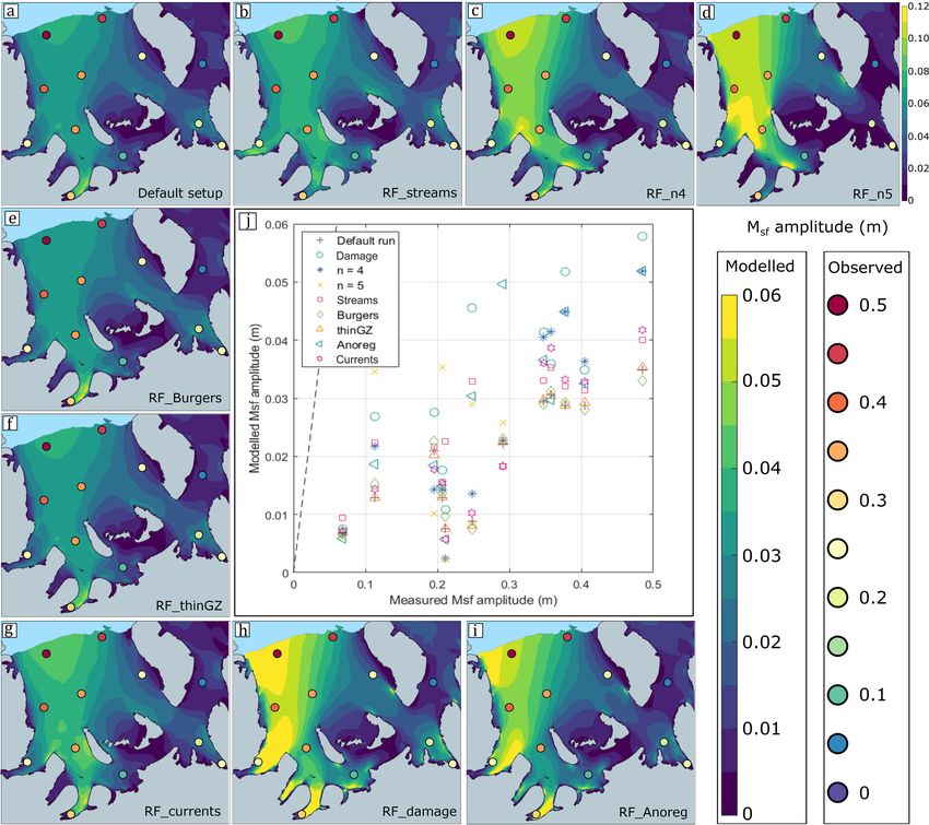
18                 S. H. R. Rosier and G. H. Gudmundsson: Modelling tidal modulation of the Filchner–Ronne Ice Shelf

2006; Marsh et al., 2013; Minchew et al., 2016; Rosier et al.,       Msf frequency whose origin is much debated (Gudmunds-
2017a). The existence of tidal effects in ice shelf flow is not      son, 2007, 2011; Thompson et al., 2014; Rosier et al., 2014,
surprising in and of itself, but the strength and nature of these    2015; Minchew et al., 2016; Robel et al., 2017; Rosier and
tidal effects is in many cases both striking and unexpected.         Gudmundsson, 2018). The model domain includes the entire
Firstly, the horizontal response of the Filchner–Ronne Ice           Filchner–Ronne Ice Shelf, and we test all the mechanisms
Shelf is strongest at a tidal frequency not found in the vertical    (as summarised below) that have been suggested in previous
tides that force it. As we discuss in more detail below, while       studies as being responsible for generating the observed tidal
the primary (vertical) ocean tidal constituents are the semidi-      response of the ice shelf.
urnal (M2 , S2 ) and the diurnal (K1 , O1 ) frequencies, the sin-       The paper is structured as follows: we begin by giving a
gle largest (horizontal) ice shelf tidal constituent is the Msf      background to ocean tides in the study area and an overview
tide with a period of 14.76 d (Rosier et al., 2017a). This Msf       of observations showing tidal modulation of ice shelf flow,
constituent is absent in the vertical ocean tides beneath the        followed by a summary of previous attempts at explaining
ice shelf, an observation that implies the existence of some         these observations. We then present our numerical model and
non-linear mechanism capable of transferring tidal energy            key results. Most of the detailed technical descriptions re-
from short (M2 , S2 , O1 , K1 ) to long (Msf ) periods. If the re-   lated to the numerical experiments and implementations of
sponse was purely a linear function of the vertical tidal forc-      different physical processes are found in several separate ap-
ing, no new frequencies could be generated. Secondly, the            pendices. We find that many of the previously proposed ex-
observed tidal flow perturbations are much stronger and more         planations, while capable of producing a response at the cor-
widespread than one might have expected based on models              rect frequencies, cannot generate a non-linear response with
that only include elastic flexure (e.g. Rack et al., 2017). The      a sufficiently large amplitude to match observations. Our pro-
long-period response gives rise to 5 % to 20 % change in flow        posed explanation, partly arrived at via a process of elimina-
velocities across the whole ice shelf. Hence, these modula-          tion, is that the tidal effects must, to a large extent, be caused
tions in flow are not limited to the elastic flexure region in       by a tidally induced migration of grounding lines coupled
the grounding zone. Finally, the shorter period tidal response       with the non-linear rheological response of ice.
can give rise to even larger changes in ice shelf velocity due
to their higher frequency. In some locations the tidal modula-       1.1   Ocean tides beneath the Filchner–Ronne Ice Shelf
tion is strong enough to cause a periodic reversal in ice flow
direction (Makinson et al., 2012).                                   Tidal models constrained by GPS observations have led
    The range of timescales over which tidal effects are seen        to accurate knowledge of vertical tidal motion beneath the
to operate suggests that studying these processes may yield          Filchner–Ronne Ice Shelf (Padman et al., 2002). Vertical
insights into both the elastic and viscous properties of ice,        tides at the grounding lines of ice streams feeding into the
thereby providing an opportunity to constrain ice rheol-             Ronne Ice Shelf are the largest in Antarctica, with a tidal
ogy over spatial and temporal scales of direct relevance to          range of up to 8 m (Fig. 1, dashed contours), making this an
ice sheet models. Furthermore, the mechanical coupling be-           ideal location to investigate tidal effects on ice shelf flow.
tween vertical ocean tides and ice flow through ice flexure             Vertical tidal motion can be split into many tidal con-
occurs in the grounding zone, a particularly important and           stituents, each with a unique period. Of these constituents,
complex part of the ice sheet where our modelling and ob-            the semidiurnal M2 (principal lunar) and S2 (principal solar)
servational efforts are often focused. Given both the com-           constituents have the largest amplitudes in this region. They
plexity of this behaviour and the difficulties in reproducing        are characterised by an amphidromic point, where their am-
it, modelling these processes can be viewed as a test of our         plitude is zero and around which they rotate, located near the
understanding of how ice flows across grounding lines and            centre of the Ronne Ice Shelf front. These two constituents
through ice shelves to the ocean.                                    have periods of approximately 12.42 and 12 h, respectively,
    Previously, Brunt and MacAyeal (2014) studied the tidal          and their combined wave envelope gives rise to the spring–
response of the Ross Ice Shelf using a viscous model. While          neap tidal cycle. This wave envelope should not be confused
the assumption of viscous rheology appears justified for stud-       with the Msf frequency, despite having the same apparent
ies of secular ice flow, this assumption is not appropriate for      “period” of 14.76 d. The Msf frequency is found in spectral
a study of processes at tidal timescales where viscoelastic          analysis of horizontal ice shelf and ice stream displacements
effects can be expected to play a significant role in the defor-     but not in the vertical tidal motion, since the semidiurnal
mation of ice (Jellinek and Brill, 1956). In this paper, we use      wave envelope contains no energy at a fortnightly period.
a full Stokes three-dimensional (3-D) viscoelastic model to          In addition to the important semidiurnal constituents, two
investigate the causes of the observed horizontal tidal mod-         diurnal constituents (O1 and K1 ) also have relatively large
ulation of ice flow over the Filchner–Ronne Ice Shelf. Our           amplitudes, increasing near the grounding lines. Unlike the
particular focus will be to investigate possible causes for both     semidiurnal constituents, these do not rotate around an am-
the strong semidiurnal modulation of ice shelf flow at the           phidromic point, and instead their phase increases approxi-
M2 frequency together with the fortnightly modulation at the         mately linearly through the region, from east to west.

The Cryosphere, 14, 17–37, 2020                                                              www.the-cryosphere.net/14/17/2020/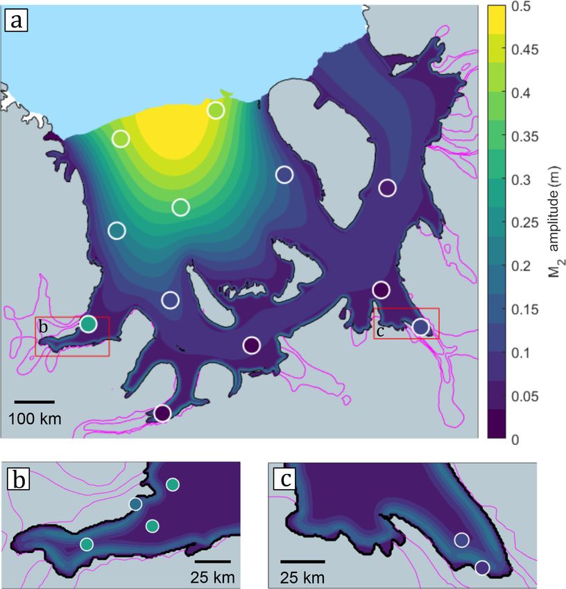
S. H. R. Rosier and G. H. Gudmundsson: Modelling tidal modulation of the Filchner–Ronne Ice Shelf                                     19

Figure 1. Map showing the Filchner–Ronne Ice Shelf and adjoining ice streams. Circular markers show locations of GPS sites and are
coloured according to Msf amplitude. The background colour map shows ice speed, grounding lines are indicated by solid black lines and
dashed contour lines show tidal range (in metres). Acronyms for glaciological features marked on the map are as follows: Evans Ice Stream
(EIS), Talutis Ice Stream (TIS), Rutford Ice Stream (RuIS), Institute Ice Stream (IIS), Moller Ice Stream (MIS), Foundation Ice Stream
(FIS), Support Force Glacier (SFG), Recovery Ice Stream (ReIS), Slessor Ice Stream (SES), Hemmen Ice Rise (HeIR), Korff Ice Rise (KIR),
Kershaw Ice Rumples (KeIR), Doake Ice Rumples (DIR) and Henry Ice Rise (HIR).

1.2   Observations of tidally modulated horizontal ice                 shelf (Makinson et al., 2012). These GPS measurements re-
      shelf displacement                                               veal strong horizontal tidal modulation at diurnal and semid-
                                                                       iurnal frequencies. During the spring tide, at sites near the
                                                                       ice front, horizontal velocity and strain varied by ±300 %
The first GPS observations to find tidal modulation of hor-            of the mean values over a tidal cycle, periodically causing
izontal ice shelf flow were made in the Ekström Ice Shelf              direction of flow to be reversed (Makinson et al., 2012). Fur-
grounding zone (Riedel et al., 1999). In the years since, sim-         ther upstream from the calving front, horizontal diurnal and
ilar observations have been made on the Brunt (Doake et al.,           semidiurnal signals were found to decay to almost zero.
2002; Gudmundsson et al., 2017a), Ross (Brunt et al., 2010),              A more recent study, which included several additional
Larsen C (King et al., 2011), and Filchner–Ronne ice shelves           GPS sites deployed for up to a year near the outlet of major
(Makinson et al., 2012; Rosier et al., 2017a) and the Mertz            ice streams feeding the Ronne Ice Shelf, found that the re-
and Langhovde glacier tongues (Legresy et al., 2004; Mi-               sponse over semidiurnal and diurnal periods increased again
nowa et al., 2019). In terms of ice shelf velocities, differ-          towards the grounding lines (Rosier et al., 2017a). Further
ent tidal constituents dominate depending on the local tidal           analysis of all available GPS data also revealed a strong Msf
regime. For example, in the Ross sea, the diurnal constituents         component in horizontal ice shelf displacements across the
(O1 and K1 ) dominate the vertical ocean tidal signal and              entire floating ice shelf (Rosier et al., 2017a). This signal had
the (horizontal) ice shelf flow response. Conversely, in the           previously been found on grounded ice streams (Gudmunds-
Weddell Sea, the semidiurnal constituents are strongest in             son, 2006; Minchew et al., 2016) and at a few locations on
both the vertical (Sect. 1.1) and horizontal motion (Makin-            the Larsen C and Brunt Ice Shelves (King et al., 2011; Gud-
son et al., 2012).                                                     mundsson et al., 2017a) but has now been found to occur over
   In this study, we focus our modelling efforts on the                a vast area and with an amplitude typically greater than had
Filchner–Ronne Ice Shelf, where we have a relatively large             been found on ice streams (Rosier et al., 2017a).
number of observations and the largest (vertical) ocean tidal
amplitudes in the whole of Antarctica. A network of nine
GPS stations made measurements spanning over a year in
locations both near the Ronne ice front and further into the

www.the-cryosphere.net/14/17/2020/                                                                 The Cryosphere, 14, 17–37, 2020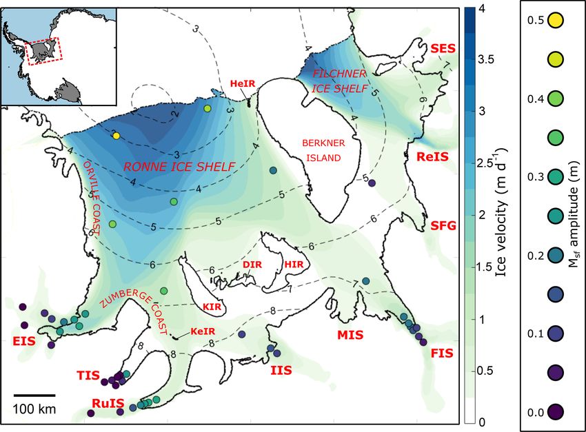
20                S. H. R. Rosier and G. H. Gudmundsson: Modelling tidal modulation of the Filchner–Ronne Ice Shelf

1.3   Proposed mechanisms for tidal modulation of ice             ing arising from grounding line migration could explain ob-
      shelf flow                                                  servations on RuIS.
                                                                     An alternative mechanism, termed “flexural ice soften-
                                                                  ing”, that results directly from the non-linear rheology of ice
With the realisation that tides can strongly modulate ice flow,   itself, was put forward by Rosier and Gudmundsson (2018).
many different mechanisms have been put forward to ex-            The authors showed that tidal bending stresses in the ground-
plain these observations. Initially, Doake et al. (2002) sug-     ing zone, which will vary in magnitude over a tidal cycle,
gested that currents beneath the Brunt Ice Shelf could be         could lead to a sufficiently large change in the effective vis-
responsible for the tidal signals found there, and this idea      cosity of ice in this region such that ice flow would be en-
was explored further by Legresy et al. (2004) and Brunt and       hanced at high and low tide and lead to modulation of ice
MacAyeal (2014). More recently, the discovery of an Msf sig-      shelf flow at the Msf frequency. Each of these non-linear
nal far upstream of the RuIS (Rutford Ice Stream) grounding       mechanisms could be playing a role in generating the ob-
line (Gudmundsson, 2006) has led to a focus on replicating        served Msf signal.
these observations (Gudmundsson, 2007, 2011; Rosier et al.,          Our main objective in this paper is to narrow down the pos-
2014, 2015; Minchew et al., 2016) and much less has been          sible causes of observed tidal motion of the Filchner–Ronne
done to understand the origin of horizontal tidal signals on      Ice Shelf by quantifying the contributions of several differ-
ice shelves.                                                      ent processes using a 3-D viscoelastic model and comparing
   The large horizontal semidiurnal modulation of the             these results with observations. In particular, we will focus
Filchner–Ronne Ice Shelf flow was discovered by Makinson          on modelling the two strongest responses observed in hori-
et al. (2012), who suggested that it could be explained by        zontal ice shelf flow: at the M2 and Msf frequencies.
an elastic response to tilting of the ice shelf as tides rotate
around the amphidromic point. On the Ross Ice Shelf, Brunt
and MacAyeal (2014) used a purely viscous model to explore        2     Methods
the effects of both tilt and currents but found that they could
not replicate GPS observations. Neither of these studies in-      In this section, we present a description of the 3-D full Stokes
vestigated longer period modulation of ice shelf flow.            viscoelastic model used to investigate tidal modulation of ice
   Efforts to understand the cause of the long period Msf sig-    shelf flow. What is described below is what we call the “de-
nal, now known to occur across many of the Antarctic ice          fault setup”. Several model experiments necessitated modifi-
shelves for which we have GPS data, require a non-linear          cations or additional features of this setup, and these differ-
mechanism (Gudmundsson, 2007). The paucity of observa-            ences are stated explicitly below. The various model versions
tions of this type on ice shelves led for some time to an im-     that arise due to these differences are listed in Table 1 and
plicit assumption that any Msf signal observed on ice shelves     each is explained in more detail in the relevant appendix.
was transmitted directly from grounded ice rather than gen-
erated in floating regions. The increasing number of observa-     2.1    Field equations
tions of the Msf signal, revealing that in at least some cases
the phase leads and amplitude are greatest downstream of          We use a 3-D full Stokes viscoelastic model in a Lagrangian
grounding lines, have made it clear that additional mecha-        frame of reference to solve for conservation of mass, linear
nisms must be at play (Minchew et al., 2016; Rosier et al.,       momentum and angular momentum (respectively):
2017a).
   One possible non-linear mechanism is that vertical tidal       Dρ
motion causes the grounding line to migrate back and forth             + ρvi,i = 0,                                           (1)
                                                                  Dt
sufficiently far as to have an effect on ice flow. Evidence of
tidal migration of grounding lines remains relatively sparse,     σij,j + fi = 0,                                             (2)
but measurements of this process have been inferred via           σij − σj i = 0,                                             (3)
remote sensing (Schmeltz et al., 2001; Brunt et al., 2011;
Milillo et al., 2017) and cryoseismicity (Pirli et al., 2018).    using the commercial finite-element analysis software
This could give rise to several non-linearities: firstly, this    MSC.Marc (MSC, 2017). In the equations listed above,
can result in the width of the ice shelf changing as the por-     D/Dt is the material time derivative, vi is the components
tion of floating ice changes over one tidal cycle (Minchew        of velocity, σij is the components of the stress tensor, ρ is
et al., 2016). In addition, the grounding line migration may      the ice density and fi is the components of the gravity force.
be asymmetric (Tsai and Gudmundsson, 2015), resulting in a        We use commas to denote partial derivatives with respect to
greater migration upstream during high tide than downstream       the spatial coordinates and the summation convention for in-
during low tide (Rosier et al., 2014). Another consequence        dices.
of tidally induced grounding line migration was explored by         Ice rheology is represented by an upper-convected
Robel et al. (2017), who suggested that changes in buttress-      Maxwell model (e.g. Gudmundsson, 2011) that relates de-

The Cryosphere, 14, 17–37, 2020                                                            www.the-cryosphere.net/14/17/2020/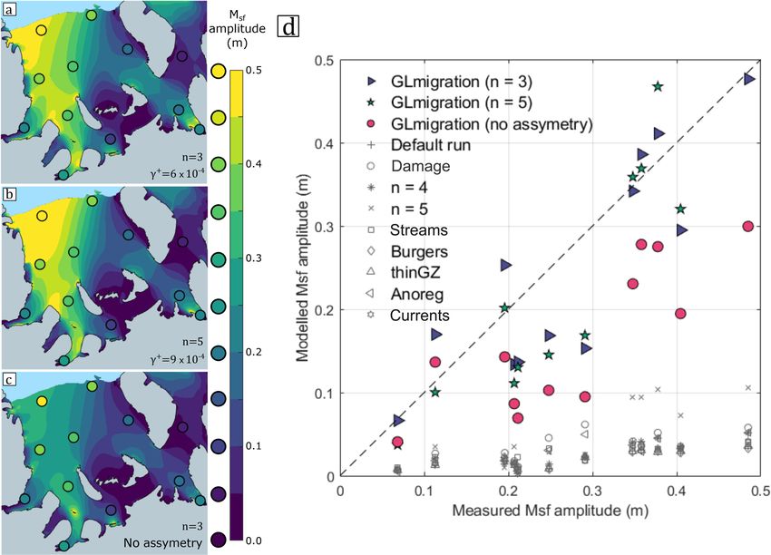
S. H. R. Rosier and G. H. Gudmundsson: Modelling tidal modulation of the Filchner–Ronne Ice Shelf                                          21

Table 1. Overview of the various model versions, including a brief description of how each one differs from the default setup and the relevant
appendix in which more details can be found.

                  Model version name    Description                                                             Appendix
                  Default setup         The default model setup, as described in the methods                    N/A
                  RF_n5                 Uses an exponent of 5 in the viscous flow law                           Appendix A
                  RF_n4                 Uses an exponent of 4 in the viscous flow law                           Appendix A
                  RF_Anoreg             Uses a rate factor of ice with no regularisation                        Appendix A
                  RF_streams            Includes grounded ice streams in the domain                             Appendix B
                  RF_damage             Includes damage effects in the ice rheology                             Appendix C
                  RF_burgers            Uses a Burgers rheological model for ice                                Appendix D
                  RF_GLmigration        Includes a parameterisation of GL migration along model sidewalls       Appendix E
                  RF_currents           Includes sub-ice-shelf tidal current drag stresses                      Appendix F
                  RF_temperature        Includes the effects of ice temperature on the rate factor of ice       Appendix G
                  RF_thinGZ             Reduces the thickness of ice in the grounding zone                      Appendix H

viatoric stresses τij and deviatoric strains eij with                    The RF_Burgers experiment uses a Burgers rheology (Ap-
                                                                         pendix D), the RF_temperature experiment makes A a func-
          1 O
ėij =      τ ij + AτEn−1 τij ,                                 (4)      tion of temperature (Appendix G) and the RF_damage ex-
         2G                                                              periment adds a damage term in the elastic component of the
                                                                         Maxwell rheology (Appendix C).
                                  p
where A is the rate factor, τE = τij τj i /2 is the effective
stress, n is the constant in the Glen–Steinemann flow law
(Steinemann, 1954; Glen, 1955), G is the shear modulus                   2.2    Boundary conditions

            E                                                            At the base of the ice shelf and along the ice front, a pressure
G=                ,                                             (5)
         2(1 + ν)                                                        is applied normal to the element faces given by
ν is the Poisson’s ratio and E is the Young’s modulus                         (
                                                                                ρw g(S(x, y, t) − z(t)) if z(t) < 0
(Shames and Cozzarelli, 1997). The superscript O denotes                 p=                                                           (9)
the upper-convected time derivative, i.e.                                       0                         otherwise,
O
τ = ∂t τ + v · Oτ − (Ov)T · τ − τ · Ov,                         (6)      where ρw is the sea water density, S(x, y, t) is the time-
                                                                         varying local sea level (Sect. 2.3) and z is the height above
and deviatoric stresses and strains are defined by                       sea level. At the ice surface, a stress-free boundary condition
           1                                                             is imposed such that
τij = σij − δij σkk ,                                           (7)
           3
                                                                         σ · n = 0,                                                      (10)
and
           1                                                             where n is the unit vector normal to the boundary. The only
eij = ij − δij kk ,                                           (8)      other boundary condition (BC) necessary in this default setup
           3
                                                                         is along the grounded sidewalls of the ice shelf domain. A
respectively, where ij are the components of the strain ten-            Dirichlet BC is imposed on nodes along the grounded edge
sor and δ is the Kronecker delta function. In all simulations            of the model, such that
we use a value for the Poisson’s ratio of 0.41, in line with
previous studies (Gudmundsson, 2011; Rosier et al., 2014,                u = uobs , v = vobs , w = 0,                                    (11)
2017a), and this choice has no effect on our results. The rate
factor is inverted for via the adjoint method implemented                where w is the vertical ice velocity and uobs and vobs are ob-
in the Úa ice flow model (Gudmundsson et al., 2012) to                   served horizontal ice velocities (Rignot et al., 2017, 2011a;
match observed surface ice velocities (Rignot et al., 2017,              Mouginot et al., 2012) and constant in time. This BC allows
2011a; Mouginot et al., 2012), as outlined in Appendix A,                for inflow from fast-moving ice streams but clamps nodes
and the resulting velocity field is shown in Fig. 2c. The model          vertically at the grounding line such that ice in the ground-
parameter choices for the default setup are shown in Ta-                 ing zone must bend to accommodate vertical tidal motion
ble 2. The rheological equations are solved implicitly with              of the ice shelf. Another result of using this Dirichlet BC
a time step that changes adaptively based on a target num-               is that the grounding line (GL) cannot migrate in these sim-
ber of iterations to reach the convergence criteria. The rheol-          ulations; however, later we will introduce a different model
ogy outlined above is modified in three of the experiments.              setup in which this constraint is loosened. We use Bedmap2

www.the-cryosphere.net/14/17/2020/                                                                    The Cryosphere, 14, 17–37, 2020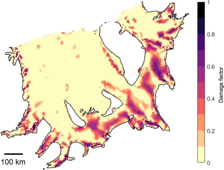
22 S. H. R. Rosier and G. H. Gudmundsson: Modelling tidal modulation of the Filchner–Ronne Ice Shelf
Table 2. List of model parameter choices for the default model ation in stress through the element. The model mesh, gen-
setup. erated using mesh2d (Engwirda, 2014), is unstructured and
refined around grounding lines and in regions of high lat-
Parameter Value Unit eral shear strain (Fig. 2a). Certain model versions necessitate
ρw 1030 kg m−3
a different mesh, but the total number of elements remains
g 9.81 m s−2 approximately the same and results in between 5 × 10⁵ and
n 3 – 1 × 10⁶ degrees of freedom.
ν 0.41 – To test the effects of mesh resolution on our model results
E 2.4 × 10⁹ Pa we ran simulations in which horizontal and vertical mesh res-
olution were doubled. The main differences in modelled Msf
amplitude are confined to the grounding zone, with a maxi-
mum change in amplitude across all nodes of 1 cm. Over the
(Fretwell et al., 2013) to define the model geometry; includ-
bulk of the shelf, the difference in Msf amplitude between
ing ice thickness, ice surface elevation and grounding line
the simulations was typically of order 1 mm or less. Simi-
position.
larly, differences in the horizontal M2 signal were limited to
2.3 Tidal forcing the grounding zone, with higher resolution resulting in sim-
ilar amplitudes but a more confined band of tidal motion at
We use the circum-Antarctic inverse model (referred to here- this frequency.
after as CATS2008a, which is an updated version of the in-
verse tidal model described by Padman et al., 2002) to force
our viscoelastic model at the ocean boundary with vertical 3 Results
tidal motion. By most measures, CATS2008a remains the
best-performing tidal model in this region (King et al., 2011). A number of different model setups were used in the course
The CATS2008a model includes 10 tidal constituents and of this study. Our strategy, whose motivation will become
we opt to force our model with the four largest constituents clear later, was to begin by attempting to reproduce GPS ob-
in the region by amplitude (M2 , S2 , O1 and K1 ), represent- servations of horizontal tidal displacements at the principal
ing the principal semidiurnal and diurnal constituents. With semidiurnal (M2 ) frequency. Once the model was able to re-
these four constituents the most important tidal features are produce these observations we subsequently searched for the
captured, such as the spring–neap cycle and the rotation of source of the fortnightly (Msf ) frequency by testing a number
tides around the Weddell Sea amphidromic point. The fort- of mechanisms and parameter combinations. Our results are,
nightly Msf signal is produced through interaction between therefore, structured in that order and we begin by present-
the M2 and S2 constituents and we include the diurnal con- ing model results at the M2 frequency. In all cases, the two
stituents to ensure that the total tidal range is close to what horizontal components of modelled surface nodal displace-
is observed. The advantage of forcing the model with only ments were processed using the UTide MATLAB package
these four constituents is to ensure that any other tidal fre- (Codiga, 2011). This state-of-the-art tidal analysis software
quencies that arise in the model must be generated through calculates amplitudes of tidal constituents using an iteratively
internal processes rather than directly from the forcing. The reweighted least-squares method and our model results are
tidal model domain uses a slightly different grounding line largely presented in terms of the semi-major axis amplitude
to that used in the model presented herein, particularly at the of each constituent.
outlet to Evans Ice Stream, so interpolation is done to fill in
areas with no amplitude or phase information in CATS2008a. 3.1 Semidiurnal (M2 ) results
2.4 Element discretisation Modelled horizontal ice shelf displacements at the M2 fre-
quency only differed slightly between all the model exper-
The finite-element mesh uses 3-D, 15-node, isoparametric iments set out in Table 1 and thus we only present the M2
pentahedrons, arranged such that the triangular faces are ori- results from the default setup. A large amplitude M2 compo-
entated in the horizontal plane (Fig. 2b). The pentahedral nent in modelled ice shelf flow is found around most ground-
shape is well suited to modelling an ice shelf in three di- ing lines and towards the ice shelf front (modelled M2 am-
mensions, since the triangular faces enable the element to plitude is shown by the main colour map in Fig. 3). The
conform to a complicated coastline geometry without an ex- maximum in the modelled M2 signal is focused around the
cessive number of elements and the relatively flat surfaces of M2 amphidromic point, near the centre of the ice shelf front,
the ice shelf are captured well with the quadrilateral faces. where the amplitude approaches 0.5 m.
The stiffness of the element is formed using 21-point Gaus- The difference between the modelled and observed re-
sian integration, and triquadratic interpolation shape func- sponse at the M2 frequency is small over the majority of
tions are used for displacements, resulting in a linear vari- the ice shelf (GPS observations of M2 amplitude are indi-
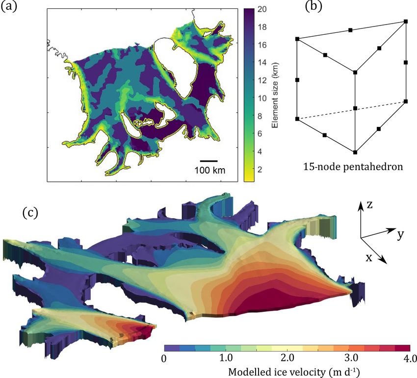
The Cryosphere, 14, 17–37, 2020 www.the-cryosphere.net/14/17/2020/S. H. R. Rosier and G. H. Gudmundsson: Modelling tidal modulation of the Filchner–Ronne Ice Shelf 23 Figure 2. Overview of the finite-element model, showing model resolution (a), the quadratic pentahedral elements used (b) and a vertically exaggerated oblique view of the model showing modelled mean ice velocity for the default setup experiment (c). cated by coloured circles in Fig. 3, using the same colour tude of the M2 effect and not its spatial variability; an in- scale as the background colour map). In particular, the bulk crease in E reduced the amplitude and vice versa for a de- signal revealed by GPS observations of increasing amplitude crease in E. Since the modelled M2 amplitude is only sensi- towards the ice front is reproduced by the model. The only tive to E, we treat it as a tuneable parameter and found that discrepancy occurs at GPS locations located near grounding a value of E = 2.4 GPa produced a very good fit to observa- lines but outside of the immediate grounding zone. GPS ob- tions. servations at these locations reveal a stronger amplitude M2 Two further model experiments were carried out to con- signal than that generated in the model, where it largely re- firm the mechanisms responsible for generating this M2 sig- mains confined to the narrow grounding zone (Fig. 3). This nal in the model. Neither of these experiments are realistic, mismatch is largest around the outlet of EIS, where mod- in the sense that the model boundary conditions are not con- elled M2 amplitude is ∼ 30 % of the value measured by GPS sistent with observations, and they only serve to better under- (Fig. 3b). Any horizontal tidal motion must decay to zero at stand the model behaviour. In the first, the vertical Dirichlet the grounding line as a result of our model BCs and so this boundary condition imposed along the sides of the ice shelf mismatch is alleviated somewhat in experiments where this was removed. In this experiment, the bulk M2 signal across constraint is removed (described later). the majority of the shelf was identical but no M2 signal was A number of model experiments were conducted specifi- generated in the grounding zone since bending effects were cally to better understand the model response at the M2 fre- removed. The second experiment set the amplitude and phase quency. Firstly, the Young’s modulus was both increased and of all tidal constituents to be the same in the whole domain decreased (between 1 and 9 GPa) to investigate how this af- (equal to the mean amplitude in this region). This stops the fects the M2 signal. This was found to only alter the ampli- ice shelf from tilting due to spatial variation in either tidal www.the-cryosphere.net/14/17/2020/ The Cryosphere, 14, 17–37, 2020
24                  S. H. R. Rosier and G. H. Gudmundsson: Modelling tidal modulation of the Filchner–Ronne Ice Shelf

                                                                       3.2.1   Flexural softening experiments

                                                                       The strength of the Msf signal generated through the flexural
                                                                       softening mechanism, as proposed by Rosier and Gudmunds-
                                                                       son (2018), is sensitive to a number of different modelling
                                                                       choices. We explore whether any of these could yield an Msf
                                                                       signal similar to observations and the results of these model
                                                                       simulations are shown in Fig. 4. Firstly, the “default_setup”
                                                                       experiment produces an Msf response whose spatial distri-
                                                                       bution appears to agree reasonably well with GPS measure-
                                                                       ments, but the amplitude is much smaller than observed
                                                                       (Fig. 4a). For example, towards the ice shelf front, where
                                                                       the Msf signal has a measured amplitude of ∼ 0.5 m, the
                                                                       modelled Msf amplitudes are about an order of magnitude
                                                                       smaller. Similarly poor numerical fit to observations is found
                                                                       around the grounding zones, where a large number of GPS
                                                                       observations exist. We thus conclude that although the de-
                                                                       fault setup produces a realistic looking spatial variation in
                                                                       Msf amplitudes, either the parameter values used are incor-
                                                                       rect, or some essential physics are missing. To identify the
                                                                       cause of the misfit, we start by investigating the sensitivity of
                                                                       the modelled response to various parameter values.
Figure 3. Amplitude of modelled horizontal ice shelf displace-
ments at the M2 frequency (background colour map) compared with
                                                                          Since it is the non-linear aspect of ice rheology that drives
GPS observations (circles). Magenta lines are 0.5 m d−1 ice veloc-     the flexural softening mechanism and gives rise to the non-
ity contours, to help identify regions of fast flowing grounded ice.   linear Msf response, we start by changing the value of the ice
Grounded ice and open ocean are coloured grey and blue, respec-        flow stress exponent. Increasing the exponent in the Glen–
tively, and ice shelves not included in the model domain are white.    Steinemann flow law from n = 3 to n = 4 (Fig. 4c) or n = 5
Panels (b) and (c) show magnified maps of EIS and FIS, respec-         (Fig. 4d; note the different colour scale used for this panel)
tively. Additional GPS sites are shown in these sub-panels that are    increases the Msf amplitude substantially; however, it is not
not shown in panel (a) for the sake of clarity.                        in a manner sufficient to match observations. We tested the
                                                                       use of the more complex Burgers rheology, which includes
                                                                       the delayed elastic response (Appendix D), but this only
amplitude or phase. With this setup the model only generates           led to a 5 %–10 % change in the Msf amplitude compared
an M2 signal in the grounding zone and there is no horizon-            to that of the default_setup (Fig. 4e). We then tried sev-
tal displacement at the M2 frequency across the main bulk of           eral different spatial distributions of the rate factor A. For
the ice shelf. These two additional experiments hence con-             example, in the “RF_Anoreg” experiment, we used a dif-
firm that the M2 signal is primarily generated through ice             ferent rate factor field to in the default setup, which was
shelf tilting with a small localised component generated near          obtained through inversion of surface velocities using the
grounding lines due to tidal flexure.                                  ice flow model Úa, but this time without any regularisa-
                                                                       tion (Appendix A). The resulting Msf amplitude is generally
3.2   Lunar synodic fortnightly (Msf ) results
                                                                       larger than the default_setup, particularly along the western
Having identified the mechanism responsible for generating             margins in the domain with a high spatial heterogeneity in
the M2 signal and having selected an appropriate value for             the rate factor field where modelled Msf amplitudes are in-
E, we now turn our attention to the Msf signal. A number of            creased by ∼ 50 % but are still much smaller than observa-
model experiments were conducted, including various differ-            tions (Fig. 4i). Thus, despite changing the value of the ice
ent processes (as outlined in Table 1) in an effort to determine       flow stress exponent n, changing the distribution of the rate
possible sources of the observed fortnightly (Msf ) modula-            factor A and using an alternative rheological model, we were
tion in flow of the Filchner–Ronne Ice Shelf. These runs can           not able to match the observed Msf amplitudes.
broadly be split into two categories; those in which the flex-            The geometry used in the default_setup model assumes
ural softening mechanism is primarily responsible for gener-           hydrostatic equilibrium to calculate ice shelf thickness from
ating an Msf signal and those that allow the GL to move and            known surface elevation, but this assumption breaks down
in which tidally induced GL migration is the primary mech-             near grounding lines where bridging stresses become impor-
anism at play.                                                         tant. Since the bending stresses that generate an Msf sig-
                                                                       nal in the default_setup are sensitive to ice thickness in the
                                                                       grounding zone, we conduct the “RF_thinGZ” experiment in

The Cryosphere, 14, 17–37, 2020                                                               www.the-cryosphere.net/14/17/2020/
S. H. R. Rosier and G. H. Gudmundsson: Modelling tidal modulation of the Filchner–Ronne Ice Shelf 25 Figure 4. Msf amplitude on the Ronne Ice Shelf for nine of the model experiments (a–i) outlined in Table 1. Note the different colour scale used for experiment “RF_n5” in panel (d). Observed Msf amplitudes from GPS observations are indicated in panel (a) by coloured circles. Panel (j) compares measured and modelled Msf amplitude at each of the marked locations for the same set of experiments. Note that in producing this figure we use an evenly distributed subset of measurements to avoid bias in areas with more measurements and thus make interpretation of the overall misfit across the entire ice shelf easier. which ice thickness is reduced in this region, as outlined in Various authors have suggested that sub-ice-shelf tidal cur- Appendix H. This change in geometry only has a small im- rents could play a role in modulating horizontal ice velocities pact on the overall Msf amplitude (Fig. 4f). Crevassing in the at tidal frequencies (Doake et al., 2002; Legresy et al., 2004). grounding zone could also reduce the effective stiffness of We use tidal currents from the CATS2008 tidal model (Pad- ice and thereby alter the magnitude of tidal bending stresses. man et al., 2002) and apply the resultant time-varying drag to In the “RF_damage” model experiment, we adopt a contin- the base of the ice shelf in the “RF_currents” experiment, as uum damage mechanics approach to simulate this effect (Ap- described in Appendix F. We ran the model with two differ- pendix C). This experiment has a more profound effect on ent drag coefficients, a “canonical” value of 3 × 10⁻³ and an effective ice stiffness and thus leads to larger changes in the “extreme” value of 3 × 10⁻² . Modelled Msf amplitude when Msf amplitude (Fig. 4h), but once again these are too small using the higher drag coefficient is shown in Fig. 4h. These to match observations. results reveal that strong tidal currents in combination with www.the-cryosphere.net/14/17/2020/ The Cryosphere, 14, 17–37, 2020
26                S. H. R. Rosier and G. H. Gudmundsson: Modelling tidal modulation of the Filchner–Ronne Ice Shelf

high drag coefficients could be locally important, increas-       migration distances are generally expected to be different and
ing Msf amplitudes in some areas by over 10 % compared            can be written as 1L+ = 1S + /γ + and 1L− = 1S − /γ − ,
to the default_setup. Overall, however, the effect of adding      where L is migration distance and the positive or negative in-
this mechanism is far too small to explain observations, even     dices indicate positive or negative vertical tidal motion. Two
when using an extreme upper-range value for the drag coef-        parameters control the distance that the GL migrates up or
ficient.                                                          downstream, γ + and γ − , which determine the upstream and
   All of the experiments described above use a constant ve-      downstream migration distance, respectively, as a function
locity boundary condition along grounding lines. As a con-        of local tidal height (1S). A more detailed description of
sequence, amplitudes of any temporal variations in ice flow       our implementation of this mechanism can be found in Ap-
go to zero towards the edges of the computational domain.         pendix E. With GL migration modelled in this way, the ex-
In order to verify that this choice of boundary condition does    periments that follow include several effects that could gener-
not significantly affect the tidal response of our model over     ate an Msf signal: asymmetric grounding line migration, tem-
the main bulk of the ice shelf, we conducted further mod-         poral variations in buttressing, and periodic narrowing and
elling experiments where the boundaries of the computa-           widening of the ice shelf.
tional domain were placed further upstream within all the            A simulation using γ + = 6 × 10⁻⁴ and γ − = γ + /7.2
main ice streams flowing into the Filchner–Ronne Ice Shelf.       yields a strong Msf signal with an amplitude of ∼0.5 m near
This setup is referred to as the “RF_streams” setup and is de-    the ice front, matching reasonably well with observations
scribed further in Appendix B. In the RF_streams setup, the       (Fig. 5a). To help put this in context, this choice of parame-
lateral extent of these additional grounded regions is chosen     ters is equivalent to a maximum upstream migration of 5 km
so that ice velocity along their boundary is approximately        (or ∼ 700 m downstream) for a positive (or negative) verti-
zero, while their upstream extent is chosen to be further than    cal tidal motion of 3 m (but note that since GL migration is
any observed tidal effects in the region (i.e. > 100 km). We      a function of local tidal amplitude, the actual migration dis-
find that around the grounding lines of major ice streams this    tance varies spatially). The migration is asymmetric (since
leads to an increase in the Msf amplitude. However, over the      γ + > γ − ), and this degree of asymmetry is within the range
majority of the shelf the differences between the two simula-     that might be expected based on geometric arguments (Tsai
tions are generally less than 10 % (Fig. 4c). Since including     and Gudmundsson, 2015). We thus find that this mechanism
the grounded ice streams greatly increases the computational      is capable of producing Msf amplitudes matching observa-
cost of running the model and we are focusing on replicating      tions.
GPS observations across the main shelf, we use this result to        We can explore what happens to the Msf amplitude if just
justify omission of grounded ice in our domain in all other       the asymmetric component of the grounding line migration
numerical experiments.                                            non-linearity is removed (i.e. γ + = γ − = 1.05 × 10⁻³ ). The
                                                                  resulting Msf amplitude with a symmetric grounding line mi-
3.2.2   Grounding line migration experiments                      gration, but the same total migration distance over one tidal
                                                                  cycle is shown in Fig. 5c. The Msf amplitude is generally
None of the numerical experiments described above were            ∼ 50 % smaller than in the asymmetric case, although it is
able to reproduce the observed Msf amplitudes and despite         still larger than experiments with no GL migration (Fig. 5d),
all our efforts modelled Msf amplitudes are only about 10 %       and certain areas such as the Kershaw Ice Rumples (KeIR)
of observed values. This suggests that hitherto we may have       generate a strong Msf signal.
not included the physical mechanism responsible for gener-           We conduct a final experiment in which we combine the
ating the observed Msf signal in our model. We stress that we     GL migration mechanism with an ice rheology in which
have, however, been able to reproduce the spatial pattern and     n = 5 in the Glen–Steinemann law. We explore this partic-
the amplitudes of the short-period (horizontal) tidal modula-     ular combination because the choice of n was found to have
tion in flow, as well as the spatial pattern in the long-period   the next largest effect on Msf amplitude (Fig. 4d), and this
tidal modulation.                                                 parameter remains poorly constrained (e.g. Cuffey and Pa-
   We now include a physical mechanism that has, until now,       terson, 2010), yet is of great importance to transient ice sheet
been missing from our modelling efforts. This mechanism in-       behaviour. Increasing the exponent in the flow law leads to
volves grounding line migration in response to tides. We use      a larger Msf signal across the shelf and thus we can obtain
the “RF_GLmigration” model version to run several experi-         an equally good match to the observed Msf amplitude with
ments that explore the role of this mechanism in generating       a lower γ + of 9 × 10⁻⁴ (Fig. 5b). In this case, upstream
the pervasive Msf signal observed on the Filchner–Ronne Ice       and downstream migration distances needed to fit observa-
Shelf. Since the amount by which the grounding line will          tions are 33 % smaller than with a choice of n = 3, but qual-
migrate is highly dependent on local bed slopes, of which we      itatively the spatial pattern of the long-period response is
have very poor knowledge, we implement this mechanism             largely unchanged.
using the simple analytical approach derived by Tsai and
Gudmundsson (2015). In essence, upstream and downstream

The Cryosphere, 14, 17–37, 2020                                                          www.the-cryosphere.net/14/17/2020/
S. H. R. Rosier and G. H. Gudmundsson: Modelling tidal modulation of the Filchner–Ronne Ice Shelf 27
Figure 5. Modelled Msf amplitude on the Ronne Ice Shelf for three variants of the RF_GLmigration model experiment. Panel (a) uses
n = 3, γ + = 6 × 10⁻⁴ and γ − = γ + /7.2, panel (b) uses n = 5, γ + = 9 × 10⁻⁴ and γ − = γ + /7.2, and, finally, panel (c) uses n = 3 and
γ − = γ + = 1.05 × 10⁻³ (i.e. no asymmetric grounding line migration). Observed Msf amplitude is indicated by the filled circles using the
same colour scale. Panel (d) compares measured and modelled Msf amplitude at each of the marked locations for runs that include the GL
migration mechanism (coloured symbols) and those previously presented that do not (grey symbols).
4 Discussion The modelled M2 amplitude was only sensitive to our
choice for the Young’s modulus (E) and the best fit to GPS
We find that strong modulation of ice shelf flow at the short- observations was found using E = 2.4 GPa. This Young’s
period M2 frequency is generated by tilting of the ice shelf, modulus can be thought of as an “effective” value, relevant
supporting the hypothesis of Makinson et al. (2012). This tilt for tidal periods, since for a viscoelastic material subjected to
occurs through a combination of phase differences in high- a periodic forcing, the Young’s modulus is a function of load-
tide times around the domain and the lower amplitude verti- ing frequency (Shames and Cozzarelli, 1997). Linear elas-
cal tides at the ice shelf front, leading to a rotating tilt vec- tic beam models have often been fitted to measurements of
tor centred around the M2 amphidromic point in the Wed- tidal flexure to obtain a wide variety of values for the effec-
dell Sea. The modelled amplitude of horizontal ice shelf dis- tive Young’s modulus of ice (Lingle et al., 1981; Stephenson,
placement at M2 frequency is very similar between all model 1984; Kobarg, 1988; Smith, 1991; Vaughan, 1995; Schmeltz
experiments that used the same elastic rheological parame- et al., 2002; Sykes et al., 2009; Hulbe et al., 2016); however,
ters and almost completely insensitive to changes in either most of these arguably mistakenly treat the resulting E as a
the viscous ice rheology or the inclusion of other mecha- material constant and furthermore they are highly sensitive to
nisms such as tidal currents and GL migration. These results local factors such as basal crevassing (Rosier et al., 2017b).
demonstrate that the short frequency modulation of ice shelf The horizontal M2 frequency ice shelf displacement in our
flow arises from simple linear elastic processes. Tidal current model is generated by strain in the main body of the shelf as
drag has previously been posited as a possible explanation it tilts due to differential tidal amplitudes. Therefore, unlike
for the modulation of horizontal ice shelf flow (Doake et al., previous studies that rely on very localised measurements,
2002; Legresy et al., 2004; Brunt and MacAyeal, 2014), a this model provides an excellent opportunity to estimate the
mechanism which we can now discount for any reasonable viscoelastic properties of ice shelves.
choice of drag coefficient. The amplitude of the modelled Msf response was also
found to be sensitive to the Young’s modulus, since this
www.the-cryosphere.net/14/17/2020/ The Cryosphere, 14, 17–37, 202028 S. H. R. Rosier and G. H. Gudmundsson: Modelling tidal modulation of the Filchner–Ronne Ice Shelf changes the bending stresses in the grounding zone. On the more complete model and a realistic geometry, together with other hand, the strength of the short period M2 signal was the numerous remote sensing and in situ GPS observations, effectively independent of any changes in viscous ice rheo- enables us to put tighter constraints on any proposed mecha- logical parameters and indeed almost any other change made nism. Model parameters that, for example, affect the spatial to the viscous model parameters. This finding justifies our pattern of secular ice flow (e.g. A and n) also impact the mod- strategy of first tuning the elastic properties of the model to elled temporal variation in ice flow generated through tidal match observed M2 response before moving on to exploring action. As a consequence, several hitherto potential mecha- the processes and parameters that play a role in generating nisms for the generation of long-period tidal modulation in the Msf signal. ice flow can now be discounted as viable explanations. Our study investigates the two mechanisms that have been Increasing the exponent n in the ice rheology increases the proposed to explain the generation of the Msf signal across an Msf amplitude, or conversely reduces the distance that the entire ice shelf: non-linear flexural ice softening and ground- grounding line needs to migrate to match the observed Msf ing line migration. We test our model results against a com- signal by 33 %. Without better knowledge of the distance that prehensive GPS dataset collected over more than a decade on grounding lines are migrating over the entire ice shelf this re- the Filchner–Ronne Ice Shelf. While the flexural ice soften- sult cannot be directly used to estimate viscous ice rheology, ing mechanism is capable of generating an Msf response, we but obtaining these data is certainly possible (e.g. Schmeltz have found that no tested combination of parameters or fur- et al., 2001; Brunt et al., 2011; Milillo et al., 2017). The mi- ther model modifications involving visco-elastic rheological gration distances we investigate in this modelling study are laws or model geometry can produce a sufficiently large am- within the range obtained by satellite estimates; in this re- plitude Msf signal to match observations through this mecha- gion, Brunt et al. (2011) identified areas in which grounding nism alone (Fig. 4). This mechanism must be responsible for lines were migrating almost 10 km over one tidal cycle. some of the observed Msf signal, since the non-linear rheol- Several features of the modelled Msf response for the ogy of ice is well established, but it cannot explain the per- RF_GLmigration experiment deserve specific mentions. Un- vasive and strong Msf signal that is observed over the entire surprisingly, there is virtually no Msf signal generated in Ronne Ice Shelf. regions where the ice shelf flows slowly, such as behind On the other hand, we do find that grounding line migra- Berkner Island and Henry Ice Rise. Somewhat more interest- tion can produce large-amplitude fortnightly modulation in ing is the lack of an Msf signal in our modelled results along ice shelf flow. Despite the relatively simple implementation the eastern coast of the Ronne Ice Shelf, despite a very large employed here, the addition of this process into the model Msf amplitude on the opposite Orville Coast (Fig. 5). This can easily produce an Msf signal that matches observed Msf is because the shear margin is located some distance from amplitude and the broadscale spatial distribution (Fig. 5a). It the grounding line (Fig. 1), meaning that migration of the would presumably be possible to obtain an exact fit to ob- grounding line is not felt by the main ice shelf (but where the servations by allowing the grounding zone geometry to vary grounding line and shear margin do coincide, at the south- spatially; however, finding the optimal geometry is a daunt- ern tip of Berkner Island, an Msf signal is generated). Upon ing inverse problem beyond the scope of this paper. closer inspection, many of the regions that generate a strong Tidally induced grounding line migration can be subdi- Msf signal coincide with areas where the shear margin is vided into several non-linear effects, which will all play a close to the grounding line. potential role in generating an Msf signal: periodic narrow- Our implementation of tidally induced grounding line mi- ing and widening of the ice shelf, reduction in basal shear gration is limited in several ways. Most importantly, without stress, reduced buttressing from ice rises and rumples, and accurate knowledge of bed geometry we have had to resort to grounding line asymmetry. With our modelling approach we assuming equal local bed slopes around all grounding lines. cannot address the reduction in basal shear stress that will In reality, it is likely that in many areas the grounding line mi- occur as the grounding line migrates upstream on major out- grates only short distances (although conversely we may be let glaciers; however, the other three have been tested using underestimating the migration in certain areas). Furthermore, the RF_GLmigration model version (Fig. 5). we do not allow the grounding line to migrate in regions of Grounding line migration has been suggested as the source inflow to the ice shelf since our analytical approach would of fortnightly modulation in ice shelf flow in two previous not yield accurate ice velocities across these grounding lines. studies, through its effects on ice shelf width (Minchew et al., However, as we are focused on matching the broadscale fea- 2016) or buttressing stresses (Robel et al., 2017). These stud- tures of the Msf signal, and localised Msf generation is found ies both showed how a horizontal Msf signal could be gen- to decay over relatively short distances (Fig. 5c), these lim- erated on an ice shelf from a vertical semidiurnal tidal forc- itations are not expected to affect our main findings. This ing but used a number of simplifying assumptions. Here, we second point is further supported by remote sensing observa- have used a 3-D model of the entire region that includes all tions, which show that the Msf signal is spatially heteroge- the stress terms and thus also flexural stresses that are ne- neous (Minchew et al., 2016). glected in the two simpler models. This combination of a The Cryosphere, 14, 17–37, 2020 www.the-cryosphere.net/14/17/2020/
S. H. R. Rosier and G. H. Gudmundsson: Modelling tidal modulation of the Filchner–Ronne Ice Shelf                                29

   Several previous studies have shown that the non-linear re-         A non-linear response to tidal bending stresses has been
sponse to vertical tidal motion which generates the Msf signal      previously proposed as a possible mechanism to explain
also leads to a change in the mean ice velocity (Gudmunds-          observed long-period horizontal motion (Rosier and Gud-
son, 2007, 2011; Rosier et al., 2014; Rosier and Gudmunds-          mundsson, 2018) and in our model this does produce the
son, 2018). Our regional model, which can broadly replicate         same general type of a response. However, our large-scale
the Msf signal across the Filchner–Ronne Ice Shelf, now al-         modelling approach using realistic geometry of the Filchner–
lows us to quantify the magnitude of this effect on an ice shelf    Ronne Ice Shelf shows that the generated long-period am-
for the first time. We ran a repeat of the RF_GLmigration ex-       plitude is too small and its spatial pattern is inconsistent
periment but with no vertical tidal forcing and compared the        with observations. We thus arrive at the lateral migration of
mean velocity in this simulation with that of our best fit to the   grounding lines over a tidal cycle as the most promising can-
observed Msf signal. We find that, averaged across the entire       didate for explaining the observations of tidal modulation on
ice shelf, ice flow is enhanced by ∼ 21 % due to the presence       Filchner–Ronne ice shelf.
of tides. Much of this tidal flow enhancement is confined to           In our model, the lateral migration of grounding lines gives
certain portions of the shelf where the local enhancement can       rise to several different non-linear mechanisms that all act
be much higher, particularly along the Zumberge and Orville         together. First, the horizontal migration distance is an asym-
coasts, i.e. ice flowing out from IIS, RuIS and EIS. This sug-      metrical function of vertical tidal amplitude (this aspect of
gests that a potentially important feedback exists between          grounding line migration arises whenever the ice-thickness
tidal amplitude and ice shelf geometry; i.e. if the ice shelf       gradient changes across the grounding line), and this is an
were to thin or retreat it would alter tides sufficiently to fur-   example of a geometrical non-linearity. Secondly, ice shelf
ther compound changes in ice flow.                                  flow is a non-linear function of width and stress for non-
                                                                    Newtonian fluid such as ice. This suggests that observations
                                                                    of tidal modulation of ice shelf flow can be utilised to extract
5   Conclusions                                                     information about rheology of ice. However, this can only be
                                                                    done if bed geometry and ice thickness across the ground-
We are able to obtain a good agreement between our model
                                                                    ing line are sufficiently well known to calculate the migra-
and observations of short-period tidal modulation in hori-
                                                                    tion distance. Alternatively, if independent observations of
zontal flow. This study, therefore, allows us to confirm the
                                                                    lateral migration of grounding lines in response to tides are
previously untested theory of Makinson et al. (2012), i.e.
                                                                    available, the migration distance can be prescribed directly,
that this behaviour arises from the linear elastic response of
                                                                    in which case the stress exponent (n) can be solved by using
ice to changes in slope resulting from the relatively high-
                                                                    a fairly simple modelling approach. Using tidal observations
frequency semidiurnal tides. We are also able to replicate,
                                                                    in this manner to extract information about ice rheology is an
here for the first time, the size and spatial pattern of the ob-
                                                                    intriguing possibility that needs to be explored further.
served long-period (i.e. longer than a day) horizontal motion
of the Filchner–Ronne Ice Shelf by including a non-linear
mechanism related to grounding line migration over tidal cy-
cles. As with other non-linear mechanisms proposed previ-
ously, this involves a non-linear energy transfer from the two
main semidiurnal tidal constituents (M2 and S2 ) to the long-
period Msf tidal constituent.

www.the-cryosphere.net/14/17/2020/                                                             The Cryosphere, 14, 17–37, 2020
You can also read