Time-lapse cross-hole electrical resistivity tomography (CHERT) for monitoring seawater intrusion dynamics in a Mediterranean aquifer
←
→
Page content transcription
If your browser does not render page correctly, please read the page content below
Hydrol. Earth Syst. Sci., 24, 2121–2139, 2020
https://doi.org/10.5194/hess-24-2121-2020
© Author(s) 2020. This work is distributed under
the Creative Commons Attribution 4.0 License.

Time-lapse cross-hole electrical resistivity tomography (CHERT) for
monitoring seawater intrusion dynamics in a Mediterranean aquifer
Andrea Palacios1,2,3 , Juan José Ledo4 , Niklas Linde5 , Linda Luquot6 , Fabian Bellmunt7 , Albert Folch2,3 ,
Alex Marcuello4 , Pilar Queralt4 , Philippe A. Pezard8 , Laura Martínez1,3 , Laura del Val2,3 , David Bosch4 , and
Jesús Carrera1,3
1 Institute of Environmental Assessment and Water Research (IDAEA), Consejo Superior de Investigaciones Científicas
(CSIC), Barcelona, 08034, Spain
2 Department of Geotechnical Engineering and Geosciences, Technical University of Catalonia (UPC-BarcelonaTech),

Barcelona, 08034, Spain
3 Associated Unit: Hydrogeology Group (UPC-CSIC), Barcelona, Spain
4 Geomodels Research Institute, University of Barcelona, Barcelona, 08028, Spain
5 Institute of Earth Sciences, University of Lausanne, Lausanne, 1015, Switzerland
6 HydroScience Montpellier Laboratory, UMR 5569, Montpellier, 34090, France
7 Cartographic and Geological Institute of Catalonia (ICGC), Barcelona, 08038, Spain
8 Geosciences Montpellier Laboratory, UMR 5243, Montpellier, 34090, France

Correspondence: Andrea Palacios (andrea.palacios@idaea.csic.es)

Received: 3 August 2019 – Discussion started: 9 September 2019
Revised: 21 March 2020 – Accepted: 25 March 2020 – Published: 30 April 2020

Abstract. Surface electrical resistivity tomography (ERT)            reflect the presence of freshwater at depth). By comparing
is a widely used tool to study seawater intrusion (SWI). It          CHERT results with traditional in situ measurements such as
is noninvasive and offers a high spatial coverage at a low           electrical conductivity of water samples and bulk electrical
cost, but its imaging capabilities are strongly affected by de-      conductivity from induction logs, we conclude that CHERT
creasing resolution with depth. We conjecture that the use           is a reliable and cost-effective imaging tool for monitoring
of CHERT (cross-hole ERT) can partly overcome these res-             SWI dynamics.
olution limitations since the electrodes are placed at depth,
which implies that the model resolution does not decrease at
the depths of interest. The objective of this study is to test the
CHERT for imaging the SWI and monitoring its dynamics at             1   Introduction
the Argentona site, a well-instrumented field site of a coastal
alluvial aquifer located 40 km NE of Barcelona. To do so, we         Seawater intrusion (SWI) increasingly affects the ever-
installed permanent electrodes around boreholes attached to          growing populations near coastlines. The inland movement
the PVC pipes to perform time-lapse monitoring of the SWI            of saline groundwater not only contaminates drinking wa-
on a transect perpendicular to the coastline. After 2 years          ter resources, but also drives other important changes in
of monitoring, we observe variability of SWI at different            ecological and hydrological cycles, thereby creating a hos-
timescales: (1) natural seasonal variations and aquifer salin-       tile environment for plants and animals that are incapable
ization that we attribute to long-term drought and (2) short-        of adapting to salinization (Michael et al., 2017; Post and
term fluctuations due to sea storms or flooding in the nearby        Werner, 2017). SWI has been studied for many years but,
stream during heavy rain events. The spatial imaging of bulk         even today, remains an open research topic because of the
electrical conductivity allows us to explain non-monotonic           complex physical, chemical, mechanical and geological pro-
salinity profiles in open boreholes (step-wise profiles really       cesses involved. The equations that govern interactions be-
                                                                     tween fresh- and seawater are well established, and models

Published by Copernicus Publications on behalf of the European Geosciences Union.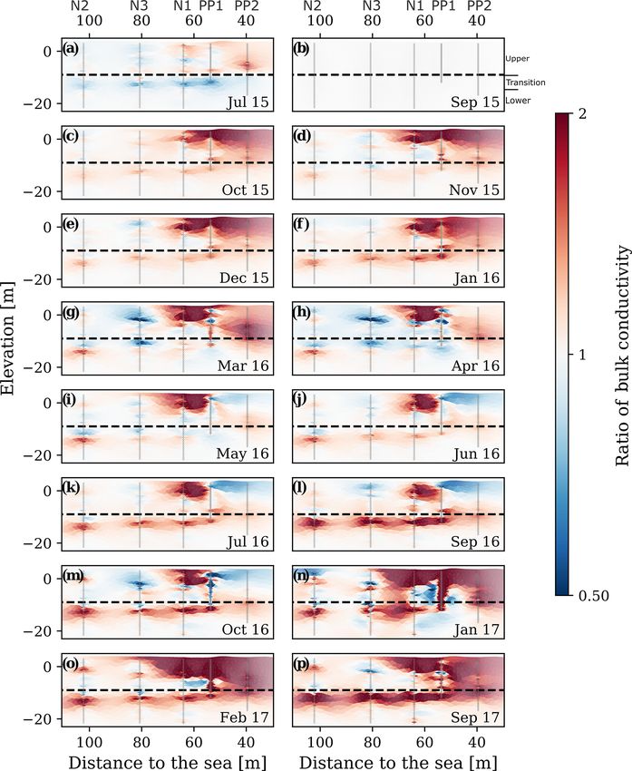
2122                                                 A. Palacios et al.: Time-lapse cross-hole electrical resistivity tomography

of simplified generic scenarios are commonly used to predict         calibration lead to important errors due to poor resolution
and assess the risks linked to SWI and to define appropriate         at depth. The computed bulk EC at depth is typically much
management strategies (Abarca et al., 2007; Henry, 1964).            lower than what we would expect from a seawater wedge
However, real field conditions are much more complex, and            with pores completely filled with seawater, which is the gen-
detailed case studies are less common in the SWI literature.         erally accepted paradigm of seawater intrusion, a seawater
   Salinity is the critical physical property to describe SWI.       wedge beneath freshwater. Paradoxically, surface ERT re-
Water salinity contrasts are so strong that salinity by itself in-   sults may be consistent with salinity profiles measured in
dicates whether water is pure freshwater, pure seawater or a         fully screened wells, which often display salinities much
mixture of both (the transition or mixing zone). The electri-        lower than that of seawater (Abarca et al., 2007). It is clear
cal conductivity (EC) of water is strongly, positively and lin-      that either measurement methods, or the current paradigm, or
early correlated with water salinity (Sen and Goode, 1992),          both, need to be revised.
so that EC represents an excellent proxy to salinity, to the            Costall et al. (2018) review some of the above issues in
point that it is often used synonymously with salinity. Electri-     their comprehensive study about electrical resistivity imag-
cal and electromagnetic geophysical measurements provide             ing of the saline water interface in coastal aquifers. Specifi-
information about the bulk or formation EC, representing             cally, they mention the scarcity of publications of time-lapse
the effective conductivity of the mixture of solid rock ma-          ERT for monitoring SWI dynamics, the low resolution of sur-
terial and the fluids contained in the pores (Bussian, 1983;         face ERT and imaging limitations related to electrode arrays.
Waxman and Smits, 1968). Pore-water electrical conductiv-            They also recommended designing optimized experiments
ity contributes to bulk electrical conductivity, which implies       suitable for the monitoring of short- and long-term salinity
that higher pore water EC results in higher bulk EC. Conse-          changes in aquifers, and in the swash zone (zone of wave
quently, bulk EC can be used as an indirect proxy measure-           action on the beach), rarely captured by land-based ERT sur-
ment of water EC, and thus of water salinity (Purvance and           veys.
Andricevic, 2000; Lesmes and Friedman, 2005). However,                  We conjecture that cross-hole ERT (CHERT) can en-
bulk EC also depends on factors such as porosity, tortuosity         hance the imaging of natural saltwater–freshwater dynam-
and constrictivity, which affect electrical current through the      ics, given that its superior resolution compared with surface-
liquid, and clay content, which may contribute to bulk EC            based deployments have been amply demonstrated in other
through mineral surface currents. This implies that detailed         related application areas (Bellmunt et al., 2016; Bergmann
site knowledge is needed to quantitatively relate bulk EC to         et al., 2012; Kiessling et al., 2010; Leontarakis and Apos-
salinity.                                                            tolopoulos, 2012; Schmidt-Hattenberger et al., 2013). Al-
   Water EC is widely used to visualize SWI (Costall et al.,         though CHERT has drawbacks (high contact resistance in
2018; Falgàs et al., 2011, 2009; Post, 2005; Zarroca et al.,         the unsaturated zone, loss of the fully non-invasive nature
2011). It is usually measured in piezometers to obtain ei-           of surface ERT and sensitivity being mainly constrained to
ther point measurements (samples) or as water EC profiles            the region between the boreholes), the benefits of this type
in fully screened boreholes. The limited sampling associated         of tomography may be larger because the resolution of the
with the former makes it inefficient to derive an image of           inversion images obtained will be high at the depths where
the typically heterogeneous salinity distribution. The latter is     changes are expected to occur. Nevertheless, there is yet no
not good practice because density-dependent flow inside the          field demonstration in the literature to test this conjecture as
borehole makes water EC profiles unrepresentative of the wa-         CHERT has never been used for monitoring SWI, most likely
ter EC in the surrounding environment (Carrera et al., 2010;         due to cost constraints, the high risk of electrode corrosion in
Shalev et al., 2009). For this reason, it is tempting to infer       saline environments, and because it typically covers a smaller
water EC from bulk EC using geophysical techniques such              investigation area than surface ERT or time-domain electro-
as electrical resistivity tomography (ERT).                          magnetics (the most common geophysical technique in salt-
   Since ERT provides more coverage than a few individual            water intrusion studies).
point measurements and is noninvasive, it has become a very             The objective of this work is to overcome the above-
common approach in SWI studies. In an inversion process,             mentioned limitations. Specifically, we test CHERT for
the ERT measurements are transformed into upscaled 2D                imaging SWI and its dynamics through time-lapse acquisi-
and 3D images of bulk EC. Many authors have used surface-            tions. To do so, a two-year monitoring experiment was con-
based ERT in real and synthetic SWI studies (de Franco et al.,       ducted at the Argentona site, located in a permeable coastal
2009; Nguyen et al., 2009; Tarallo et al., 2014; Beaujean            alluvial aquifer in northeast Spain.
et al., 2014; Huizer et al., 2017; Sutter and Ingham, 2017;
Goebel et al., 2017), with the results being negatively af-
fected by the low resolution of the images at depth. As a            2   The Argentona site
manifestation of this problem, Huizer et al. (2017), Beau-
jean et al. (2014) and Nguyen et al. (2009) showed that us-          The Argentona site (Fig. 1) is located at the mouth of the
ing ERT-derived salt-mass fraction for solute transport model        “Riera de Argentona” (Argentona ephemeral stream), some

Hydrol. Earth Syst. Sci., 24, 2121–2139, 2020                                      www.hydrol-earth-syst-sci.net/24/2121/2020/
A. Palacios et al.: Time-lapse cross-hole electrical resistivity tomography                                                             2123

Figure 1. (a) Location map of the Argentona site, some 30 km northeast of Barcelona, Spain. (b) Field spread of the Argentona site,
installed piezometers (black dots), piezometers equipped with electrodes (yellow dots), surface ERT and CHERT transects. (c) Vertical cross
section showing piezometers with screened depth, and location of the 36 electrodes in each well and stratigraphic correlation (modified from
Martínez-Pérez et al., 2018). Two sandy aquifers are loosely separated by a silt layer at 12 m depth. The semiconfined aquifer is underlaid by
weathered granite.

30 km northeast of Barcelona. The field site covers an area                 We have installed 16 piezometers in a cross-shaped distri-
of some 1500 m2 and the mean elevation is 3 m. The Argen-                bution with the longest axis being oriented perpendicularly
tona stream only flows during heavy rainfall episodes that               to the coastline (Fig. 1a). These include four nests (N1–N4)
occur mainly in autumn. The climate is sub-Mediterranean.                of three piezometers with depths of 15, 20 and 25 m (N115,
According to data from the Cabrils weather station, located              N120, N125, etc.), screened over 2 m at the bottom. The
7 km northeast of the site, the mean annual precipitation since          distance from the closest piezometer (PP20) to the coast-
2000 is 584.1 mm. Compared to most Mediterranean areas,                  line is almost 40 m. The field site is located on a coastal
the precipitation is more evenly distributed throughout the              alluvial aquifer that overlies a granitic basement (Fig. 1b).
year, with the rainiest seasons being spring and autumn.                 Core analyses reveal that the sediments are mostly unconsol-
                                                                         idated. Martínez-Pérez et al. (2018) identify two sequences,

www.hydrol-earth-syst-sci.net/24/2121/2020/                                             Hydrol. Earth Syst. Sci., 24, 2121–2139, 2020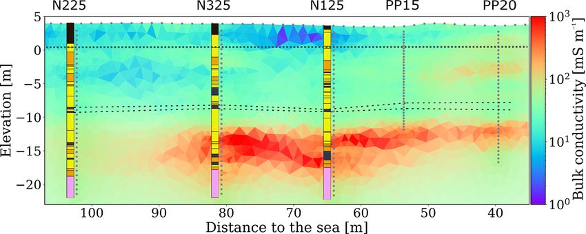
2124                                              A. Palacios et al.: Time-lapse cross-hole electrical resistivity tomography

located above and below a silt layer at −9 m a.s.l. The up-       by fixing constraints about the resistivity structures during
per and lower sequences display a fining-upward pattern.          the inversion procedure. In the Argentona site, the aspect ra-
The granitic basement was found at −17 to −18 m a.s.l. in         tio for the different borehole pairs considered ranges from
piezometers N225, N325 and N125, with signs of intense            0.6 to 0.8. Further details on the setup and installation are
weathering. A well-correlation profile was built from core        described by Folch et al. (2020).
descriptions supported by gamma-ray and induction logs.              When performing ERT, we measure an “apparent” resis-
The silt layer at −9 m a.s.l. appears to be continuous along      tivity that depends on the geometry of the acquisition. The
the main transect between piezometers N225 and PP20. Its          apparent resistivity is related to measured electrical resis-
continuity, especially towards and below the sea and its low      tances:
permeability nature are yet to be defined. The present 2D                    V
conceptual model of the site is simple and several questions      ρapp = K ,                                                  (1)
                                                                             I
remain unanswered: is the silt layer continuous and imper-
                                                                  where ρapp is the apparent resistivity, K is a geometric factor
vious or is a significant water flow passing through it? Is
                                                                  that depends on the electrode array and site characteristics, V
the weathered granite an aquitard or another permeable unit
                                                                  is the voltage between two electrodes measured during cur-
given its strongly weathered nature? (see for example De-
                                                                  rent injection and I is the magnitude of the current flowing
wandel et al., 2006). One of the goals of our time-lapse
                                                                  between another pair of electrodes. Any electrode configu-
CHERT investigations is to contribute to answering these
                                                                  ration or array can, in principle, be used to perform ERT at
open questions and improve the conceptual understanding of
                                                                  the surface or between boreholes. For surface ERT, there are
the site.
                                                                  many well-established array types, such as Wenner, Schlum-
                                                                  berger, dipole–dipole or pole–pole. For CHERT, several stud-
                                                                  ies have sought to determine the most informative and cost-
3   CHERT experimental setup
                                                                  effective arrays for monitoring dynamic processes (Bellmunt
                                                                  et al., 2012; Zhou and Greenhalgh, 2000). Bellmunt et al.
The objectives of the time-lapse CHERT experiments are to
                                                                  (2016) suggest that it is better to use different configura-
image SWI in order to improve the geological conceptual
                                                                  tions (dipole–dipole, pole–tripole and Wenner) with differ-
model, and to infer SWI dynamics. This requires installing
                                                                  ent sensitivity patterns in order to obtain the maximum infor-
metal electrodes in a corrosive saline environment, in which
                                                                  mation about the subsurface. Moreover, given the corrosive
electrolysis due to current injection further accelerates the
                                                                  environment in which the steel electrodes were installed, we
corrosion process and limits the lifetime of the installation.
                                                                  decided to maximize the number of data measurements to
Therefore, addressing corrosion was one of the main con-
                                                                  ensure enough repeatability for the time-lapse inversion. The
cerns when designing the system and planning the monitor-
                                                                  different configurations used were already described and as-
ing experiments. The impact of corrosion on the electrode-
                                                                  sessed by Zhou and Greenhalgh (2000) and Bellmunt et al.
functioning was tested in the laboratory before field deploy-
                                                                  (2016). Figure 2b shows the electrode configurations used at
ment. The parts that are most sensitive to corrosion are the
                                                                  the Argentona site: dipole–dipole, pole–tripole and Wenner.
connection points between the mesh electrodes and the cop-
                                                                  Note that these data are acquired sequentially by considering
per cables that bring current. Our strategy to delay corro-
                                                                  one pair of neighboring boreholes at a time.
sion at the connection points was to tie together the mesh
                                                                     We use an optimized survey design that allows more than
and the cable, and to cover the connection point by a double
                                                                  5800 data points to be acquired in less than 30 min. After the
silicone layer to prevent contact with water. In the labora-
                                                                  installation of the electrodes around the casings (36 at each
tory, the electrodes showed signs of corrosion after 500 h of
                                                                  borehole), the data acquisition process was straightforward,
full contact with saline water (55 mS cm−1 ), under a constant
                                                                  with no need for large additional costs in maintenance or hu-
current injection of 1 A at a frequency of 3 Hz. In our setup,
                                                                  man working time. The equipment used was a Syscal Pro
stainless-steel mesh electrodes were permanently attached to
                                                                  multi-channel (10-channel) system from IRIS instruments
the outside of the seven deepest PVC piezometers (Fig. 2a).
                                                                  with 72 electrodes. The current injection time was 250 ms,
When conducting a CHERT, the injected current is less than
                                                                  and stacking of up to six measurements was done to meet
1 A and the time of injection is a fraction of a second. Based
                                                                  data quality requirements. It took 2 h to complete the four
on these laboratory test results, it was suggested that the in-
                                                                  CHERT acquisitions needed to cover the whole 2D transect
strumentation would last for at least 2 years, which was the
                                                                  from boreholes N225 to PP20. The combination of four such
minimum desired duration of the experiment.
                                                                  sections are referred to as a complete CHERT.
   All piezometers have 36 electrodes and the distance be-
tween electrodes is 70, 55 and 40 cm in the 25, 20 and 15 m
depth piezometers, respectively. Numerical simulations by         4   Processing and inversion methods
al Hagrey (2011) suggest that satisfactory resolution can be
achieved using aspect ratios (horizontal distance between the     A total of 16 time-lapse datasets were collected during
boreholes and their depths) of up to 2 for different scenarios    2 years (five in 2015, eight in 2016, and three in 2017), cor-

Hydrol. Earth Syst. Sci., 24, 2121–2139, 2020                                  www.hydrol-earth-syst-sci.net/24/2121/2020/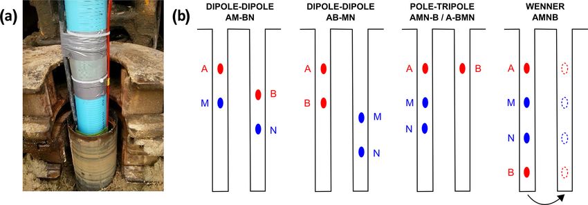
A. Palacios et al.: Time-lapse cross-hole electrical resistivity tomography                                                         2125

Figure 2. (a) Stainless-steel meshes (electrodes) permanently fastened around PVC piezometers for the time-lapse CHERT experiment
during piezometer installation. (b) Electrode configurations used in the survey. A total of 5843 measurements are recorded per CHERT in
less than 30 min. Data are acquired sequentially by considering one pair of neighboring boreholes at the time. Four CHERT acquisitions are
needed to build a complete CHERT, the whole 2D transect from boreholes N225 to PP20.

responding roughly to a complete CHERT every 90 d. This                eling Library) (Rücker et al., 2017). The inversion algorithm
relatively low sampling interval was partly motivated to de-           inverts the log-transformed apparent resistivities, into a 2D
crease corrosion of the electrodes due to repeated current in-         log-transformed electrical resistivity distribution. The objec-
jections.                                                              tive function to minimize is
   Data pre-processing was needed to remove anomalous and
erroneous data points prior to imaging. Comparison of nor-             φ = φd + λφm = ||C−0.5
                                                                                         d    1d||n + λ||C−0.5  n
                                                                                                          m 1m|| ,                    (2)
mal and reciprocal measured resistances is a common tech-
                                                                       where φd is the data misfit term, 1d = d − f (m) is the vec-
nique for appraising data errors (LaBrecque et al., 1996;
                                                                       tor containing data residuals, d is a vector containing field
Slater et al., 2000; Koestel et al., 2008; Oberdörster et al.,
                                                                       data, f (m) is the forward response of the geoelectrical prob-
2010; Flores-Orozco et al., 2012). We follow the strategy
                                                                       lem using model m and n is the order of the norm. In order
proposed by Bellmunt and Marcuello (2011) for the quality
                                                                       to make the inversion less sensitive to data outliers, we apply
control of the data based on the comparison between normal
                                                                       a L1-norm mimicking scheme to the data misfit term using
and reciprocal measurements. We chose a threshold of 10 %
                                                                       iteratively reweighted least squares (ILRS) (Claerbout and
difference between the normal and reciprocal data in order
                                                                       Muir, 1973). We assume uncorrelated data errors, so Cd−0.5
to keep the measurement. Furthermore, the electrical con-
                                                                       is a diagonal matrix with entries containing the inverse of
tact resistance between the electrodes and the subsoil was
                                                                       the relative resistance errors. A relative error model with a
checked before each data acquisition. Although the specific
                                                                       3 % mean deviation is further assumed. 1m = m − mref is
values of each pair of electrodes were not recorded, they were
                                                                       the vector being penalized in the model regularization, with
low in general. The deepest electrodes, in contact with the
                                                                       m the vector of estimated parameters and mref a vector of ref-
SWI, had contact resistance values in the order of 1 k and
                                                                       erence parameters. C−0.5
                                                                                             m    is the model regularization matrix.
the ones closer to the surface had values of a few tens of kilo-
                                                                       Smoothness operators are frequently used but are not suitable
hms. Pseudo-sections of the apparent resistivities are easily
                                                                       for capturing the sharp resistivity changes expected at the in-
created for surface ERT surveys, but there is no correspond-
                                                                       terface of the saltwater intrusion. We have chosen to define
ing visualization technique for CHERT surveys. Instead, we
                                                                       Cm as a geostatistical operator (Chasseriau and Chouteau,
plot geometric factors, apparent resistivities and data errors
                                                                       2003; Linde et al., 2006; Hermans et al., 2012), containing
versus data number, to identify electrode configurations with
                                                                       site-specific information about how the resistive bodies are
anomalous values. Clearly, for time-lapse studies it is impor-
                                                                       expected to correlate in space. Hermans et al. (2016) pro-
tant to ensure that changes observed are due to subsurface
                                                                       vide an example of how the inclusion of covariance informa-
processes, and not to changes in the survey setup. Conse-
                                                                       tion in ERT inversion improves the imaging of the target in
quently, the 16 datasets were scanned and compared to keep
                                                                       terms of shape and amplitude, creating more realistic images.
only identical electrode configurations.
                                                                       For this purpose, we use an exponential covariance model
   For inversion, we make the common assumption that the
                                                                       implemented in pyGIMLi by Jordi et al. (2018). The spa-
bulk EC distribution is constant in the direction perpendicu-
                                                                       tial support of the geostatistical operator helps to reduce the
lar to the complete CHERT transect. The corresponding 2.5D
                                                                       tendency of anomalies being clustered around the electrode
electrical inverse problem is solved on an unstructured mesh
                                                                       region where sensitivities are high. The parameters used in
with tetrahedral elements using BERT (Boundless Electri-
                                                                       the covariance model were chosen in agreement with the ex-
cal Resistivity Tomography) (Rücker et al., 2006; Günther
                                                                       pected groundwater processes. Pore water is expected to flow
et al., 2006) and pyGIMLi (Generalized Inversion and Mod-
                                                                       through the horizontal layers shown in the stratigraphic cor-

www.hydrol-earth-syst-sci.net/24/2121/2020/                                          Hydrol. Earth Syst. Sci., 24, 2121–2139, 2020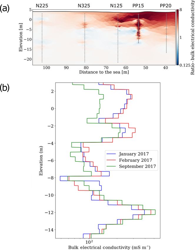
2126                                                  A. Palacios et al.: Time-lapse cross-hole electrical resistivity tomography

relation, so the variations that we expect to observe will be         ence model mref and d ref is the data vector of reference time
more correlated in the horizontal direction than in the verti-        t ref .
cal direction. The integral scales in the horizontal and vertical         The reference model for time-lapse inversion was built
direction are 10 and 2 m respectively, the anisotropy angle is        by inverting data from a complete CHERT and surface ERT
90◦ , and the variance of the logarithm of the resistivities was      from 8 September 2015. The surface ERT dataset consists of
set to 0.25. The detailed description of this type of covariance      1600 data points acquired along the transect shown in Fig. 1a.
model is found in, for example, Kitanidis (1997).                     We used the Wenner–Schlumberger configuration with 72
   The minimization of φ is performed iteratively using the           electrodes and a 1.5 m electrode spacing. Inversion results
Gauss–Newton scheme. We start the inversion with a homo-              are displayed in the next section in terms of bulk electrical
geneous model corresponding to the average apparent resis-            conductivities, σb (the reciprocal of resistivities ρb ).
tivity. In Eq. (2), λ is the regularization parameter. We apply
an Occam-type inversion, in which we seek the smallest φm
while fitting the data (Constable et al., 1987). We set λ to a        5     Results
high value at the first iteration and decrease it by 0.8 in each
subsequent iteration. The iterative process is stopped when           5.1    Reference model
the data are fitted to the noise level.
   To study variations in time, the simplest approach consists        Inversion results of data used to establish the reference model
of independently inverting each dataset to analyze the evo-           are shown in Fig. 3. We display the bulk EC model obtained
lution of changes. This approach may work when changes                by the inversion of the CHERT and surface-based ERT data
are large, but it is not considered state-of-the-art because in-      (Fig. 3a), the result obtained when only considering the com-
version artifacts tend to be time independent (though not al-         plete CHERT (Fig. 3b) and only the surface ERT (Fig. 3c)
ways; see discussion by Dietrich et al., 2018) and may mask           next to the calculated coverages for each model (Fig. 3d–f).
actual changes. Singha et al. (2014) review time-lapse in-            The bulk EC model obtained from the surface ERT campaign
version as a way to impose a transient solution constraint            shows resistive layers in the first 5 to 10 m below the land sur-
through the analysis of differences or ratios in the data             face, while the model obtained from the complete CHERT
(Daily et al., 1992; LaBrecque and Yang, 2001), through               data alone is unable to resolve them. The complete CHERT,
the differentiation of multiple individual inversions (Loke,          however, shows high conductive anomalies at depth. Also,
2008; Miller et al., 2008), or through temporal regulariza-           the magnitude of the bulk EC below −10 m a.s.l. is higher
tion (Karaoulis et al., 2011). Daily et al. (1992) introduced         in the complete CHERT model. These results confirm the
the ratio inversion, in which data are normalized with re-            expectations derived from the literature described in the in-
spect to a reference model represented by a homogeneous               troduction. Surface ERT is unable to accurately image the
half-space. The method allowed qualitative interpretation of          magnitude of saline regions at depth. Figure 3e and f dis-
resistivity changes, but made quantitative interpretation dif-        play the coverage of the CHERT and surface ERT acquisi-
ficult. This motivated “cascaded inversion” (Miller et al.,           tions computed using the cumulated sensitivity. The maxi-
2008), which consists of selecting as reference model the             mum coverage is attained near the electrodes. By combining
result of an initial inversion or baseline dataset. This ap-          the two datasets, the inverted bulk EC model has high sensi-
proach removes the effects of errors and yields more reli-            tivity near the surface and at depth. The complementarity of
able sensitivity patterns (Doetsch et al., 2012). The differ-         the two surveys is well illustrated in Fig. 3d. For the refer-
ence inversion by LaBrecque and Yang (2001) assumes that              ence model of the time-lapse inversion, we chose the inver-
the changes from one acquisition to another are small, but            sion result from the complete CHERT dataset and the surface
this is not the case throughout the 2 years of monitoring at          dataset (Fig. 3a).
the Argentona site. In the newest approaches, a 4D active                Figure 4 shows the reference model with the site strati-
time-constrained inversion is applied simultaneously to all           graphic correlation. The estimated bulk electrical conductiv-
datasets (Karaoulis et al., 2011), penalizing differences be-         ity ranges from 1 to 1000 mS m−1 . A resistive layer of less
tween models. Although this is the most novel procedure for           than 5 mS m−1 is visible in the top 3 m, starting 60 m from
time-lapse inversion, it is computationally demanding. We             the sea. This layer with low bulk EC is caused by the un-
have decided to apply the “ratio inversion”, solving for the          saturated zone; it coincides with the depth to groundwater
updates of a reference model and thereby allowing us to ac-           (gray dotted line in Fig. 4) that usually varies between 0
count for the leading non-linear effects.                             and 0.5 m a.s.l. The thickness of the unsaturated zone is re-
   For data at time-lapse t,                                          solved thanks to the surface ERT data. The bulk EC grows
                                t                                  to a mean value of 50 mS m−1 below the water table in the
                             ref d

φd = ||C−0.5
           d     d t
                     − f   m            ||n ,                 (3)     shallow aquifer from 0 to −10 m.a.s.l. Conductivity grows
                                 d ref                                further, exceeding 500 mS m−1 , below −10 m.
where d t is the data vector at time t, f (mref ) is the calculated      Bulk electrical conductivity values above 200 mS m−1 can
forward response of the geoelectrical problem using a refer-          here be conclusively attributed to the presence of seawater in

Hydrol. Earth Syst. Sci., 24, 2121–2139, 2020                                         www.hydrol-earth-syst-sci.net/24/2121/2020/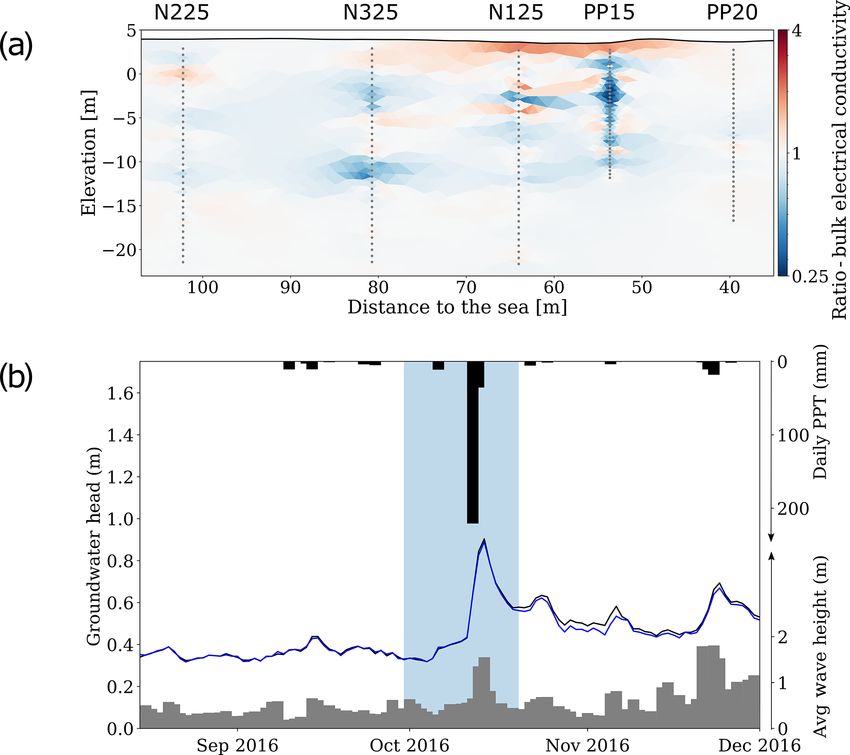
A. Palacios et al.: Time-lapse cross-hole electrical resistivity tomography                                                              2127

Figure 3. Bulk electrical conductivity models obtained by the inversion of the CHERT and surface-based ERT data (a), the result when only
considering the complete CHERT (b) and only the surface ERT (c) with the corresponding calculated coverages for each model (d–f). The
complete CHERT model shows conductive anomalies (in red), which are not shown by the surface ERT model. The inversion of both datasets
combines the coverages and yields an image with higher resolution near the surface and at depth (d).

Figure 4. Result from the inversion of surface and cross-hole ERT (dataset from 8 September 2015). Stratigraphic columns are shown to
relate stratigraphic units with bulk conductivities. Gray dots represent the electrodes around the boreholes and on surface. The gray dashed
line indicates the approximate groundwater table. The black dashed line indicates the silt layer. This cross section is used as reference model
in the time-lapse inversion.

the pore space. We see an upper conductive anomaly of some                the bottom part of Fig. 4, bulk EC decreases where the top of
100 mS m−1 in the unconfined aquifer above −5 m a.s.l. to-                the granite is found in piezometer N125.
wards the sea (from 35 to 50 m to the coast). We attribute                   The reference model and stratigraphic units provided in-
this anomaly to beach sediments saturated with a mixture of               sights pertaining to the interpretation of subsurface pro-
fresh and saline water. The upper anomaly vanishes inland                 cesses. Time-lapse changes will help confirm whether con-
before piezometer PP15. The second conductive anomaly,                    ductivity anomalies in the reference model are related to fluid
below −10 m a.s.l., extends from 35 to 90 m to the coast, and             dynamics or to geologic structures.
it vanishes before reaching piezometer N225. Poor imaging
resolution is not expected at this depth, so we must consider             5.2   Time-lapse results
the possibility that lithological heterogeneity or lower water
salinity causes the change in bulk EC in the lower aquifer. In            Figure 5 shows the time evolution of the data percentage that
                                                                          satisfies the constraints on data quality (less than 10 % per-
                                                                          cent of difference between normal and reciprocal measure-

www.hydrol-earth-syst-sci.net/24/2121/2020/                                             Hydrol. Earth Syst. Sci., 24, 2121–2139, 2020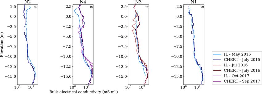
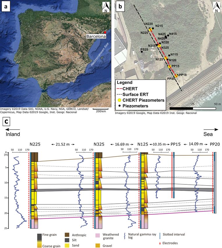
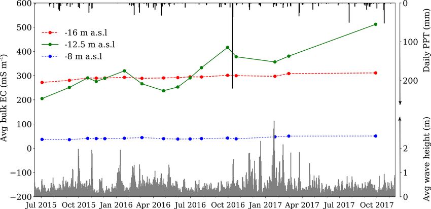
2128                                                  A. Palacios et al.: Time-lapse cross-hole electrical resistivity tomography

Figure 5. Percentage of accepted data points in each CHERT, after quality control during data pre-processing. Note the decrease in the
amount of accepted data with time, most likely due to corrosion of the electrodes, particularly in the PP20-PP15 panel, which is located the
closest to the sea.

ments). The panel between boreholes PP20 and PP15 is the                ratio images between nest N3 and borehole PP20. This is the
one that suffers the most from discarded data, likely due to its        largest anomaly captured by the experiment in size and mag-
proximity to the coast, and it is the zone where lower resistiv-        nitude. In the last ratio image between September 2017 and
ities cover a thicker vertical zone. The decrease in data qual-         September 2015 (Fig. 6l), the increase in bulk EC in the study
ity with time is probably related to corrosion processes of the         area is clearly observed.
electrodes in contact with marine water. The quality control               We analyze the origins of long-term and short-term
after each acquisition, plus the identical geometry constraint          changes described in the previous paragraph by correlating
for the time-lapse inversion, reduced the dataset to 2677 iden-         them with precipitation and wave activity data. The precip-
tical measurements that were extracted from each complete               itation and the wave activity data are here used as a proxy
CHERT.                                                                  to indicate the likely timing when a significant freshwater
   Time-lapse results are displayed in Fig. 6 as the ratio be-          recharge occurred and when water from large waves might
tween each bulk EC model and the bulk EC of the refer-                  have formed seawater ponds at the surface.
ence model (September 2015). The color scale in the fig-                   Figure 7 displays the average conductivity of the inverted
ure varies from a twofold increase (dark red) to a decrease             model at −8, −12.5 and −16 m a.s.l. In this figure we also
by half (dark blue) in bulk EC with time. The color scale               display daily precipitation data from the Cabrils Station, lo-
does not show the minimum and maximum magnitude of                      cated 7 km northeast of the site. Precipitation data (inverted
the variations; it was chosen to highlight major changes in             y axis) show two relevant features: (1) important precipi-
the 2 years of monitoring. In the imaging process, the use              tation events can occur in one day (e.g., 220 mm in Octo-
of a geostatistical operator in model regularization helped             ber 2016); (2) the rainiest periods during the 2 years of moni-
in removing the boreholes’ footprint in the bulk EC mod-                toring consistently occurred in the fall and spring. The winter
els, but these remain in the ratio images due to the high sen-          and summer of 2016 were the driest periods. Wave-related
sitivity of the method near the electrodes. Figure 6a (ratio            data (normal y axis) are obtained from a numerical model
of September to July 2015 ECs) shows an increase in bulk                called SIMAR 44 (Pilar et al., 2008). The numerical model
EC during summer 2015. That is, EC is smaller in July than              is calibrated using data from wave buoys distributed along
in September, which suggests advancement of salinity. From              the Catalan coast. Wave numerical models have limitations
October 2015 to March 2016 (Fig. 6c–g) an increase is suc-              and tend to underestimate wave height near the coast, but
cessively observed near PP20, reaching 70 m from the sea. In            they give general insights about the wave activity (WAMDI
March, April and May 2016 (Fig. 6g–i), a decrease in bulk               Group, 1988). In Fig. 7, we show the significant wave height
EC is observed in both aquifers. Complete CHERT values                  from the numerical model. Significant wave height (Hs ) is
from June 2016 to September 2017 (Fig. 6j–l) show succes-               defined as the average height of the highest one-third of
sive increases in the conductivity of the semiconfined aquifer,         waves in a wave spectrum (Ainsworth, 2006), and it is the
below −10 m a.s.l. In 2017 (Fig. 6m–l), a highly conductive             most commonly used parameter because it correlates well
anomaly reappears in the upper-right part of the time-lapse             with the wave height that an observer would perceive. The

Hydrol. Earth Syst. Sci., 24, 2121–2139, 2020                                          www.hydrol-earth-syst-sci.net/24/2121/2020/
A. Palacios et al.: Time-lapse cross-hole electrical resistivity tomography                                                           2129

Figure 6. Results from the time-lapse inversion of 16 complete CHERT acquired over 2 years (July 2015 through September 2017). Images
display the ratio of bulk electrical conductivity with respect to September 2015 (a brownish area implies higher EC and, therefore, salinity
than in September 2015). The silt layer is indicated with a dashed line. Note the increase in bulk EC in the upper-right side (< 80 m of
distance to the sea), and along a line just below the silt layer, indicating a rise in the saltwater interface.

wave data show increased wave heights in Autumn 2015,                   the shallow (bulk EC around 20 mS m−1 ) and greater (some
January 2016 and winter 2017. These periods correspond to               300 mS m−1 ) depths.
the appearance of a superficial conductive anomaly in the up-              In order to assess the impact of a heavy rain event at
per part of the time-lapse images.                                      the site, we have computed the ratio of the CHERT bulk
   The plots of average bulk EC in Fig. 7 capture the evo-              EC models from 30 September and 21 October 2016, 11 d
lution of the conductivity in the unconfined and the under-             before and 9 d after the heavy 220 mm precipitation. The
lying semiconfined aquifer over time. The mean bulk EC                  color scale chosen for the Fig. 8a differs from previous
of the upper portion of the lower aquifer (at −12.5 m a.s.l.)           figures to improve visualization of the bulk conductivity
displays a more than twofold increase (from 200 to more                 variations. Figure 8a displays the conductivity ratio image,
than 500 mS m−1 ) in the 2 years of monitoring. We can also             which reveals a decrease in the conductivity throughout the
observe cyclic variations throughout the year. In contrast,             saturated zone, both above and below the −10 m a.s.l. silt
both fluctuations and overall variation are very small at both          layer, and an increase in the unsaturated zone, above the
                                                                        0 m a.s.l., between nest N3 and PP20. No difference is ob-

www.hydrol-earth-syst-sci.net/24/2121/2020/                                           Hydrol. Earth Syst. Sci., 24, 2121–2139, 2020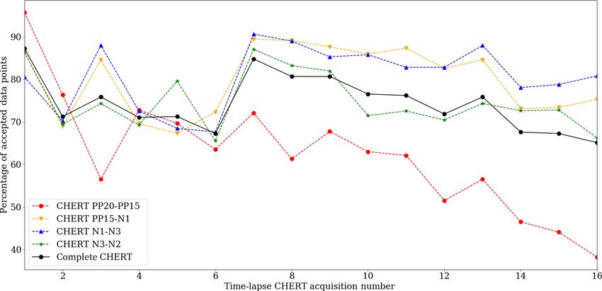
2130                                                  A. Palacios et al.: Time-lapse cross-hole electrical resistivity tomography

Figure 7. Average conductivities extracted from the inverted models, at −8 m a.s.l. (blue), −12.5 m a.s.l. (green) and −16 m a.s.l. (red).
Precipitation (PPT) data from Cabrils station and simulated significant wave height time series are displayed. The points indicate times
of CHERT campaigns. Note that acquisitions were made before and after the 220 mm precipitation event of 12 October 2016. Significant
seasonal fluctuations and an overall increase in EC can be seen in the upper part of the semiconfined aquifer (elevation of −12 m a.s.l.) but
are negligible in the lower portion of both the shallow unconfined aquifer (−8 m a.s.l.) and the semiconfined aquifer (−16 m a.s.l.).

Figure 8. (a) Ratio between the bulk electrical conductivity model of 30 September and 21 October 2016. The heavy rain occurred on
12 October 2016. The image shows a decrease in conductivity in the unconfined and semiconfined aquifer and a conductivity increase in the
unsaturated zone on both sides of nest N1. The decrease in conductivity observed along borehole PP15 is attributed to freshwater infiltration
due to borehole construction. (b) Time series of groundwater level in boreholes N115, average significant wave height (gray bars) and
precipitation (black bars). Highlighted is the heavy rain event of 220 mm that occurred on 12 October 2016. The event was accompanied
with an increase in groundwater level and in significant wave height.

Hydrol. Earth Syst. Sci., 24, 2121–2139, 2020                                           www.hydrol-earth-syst-sci.net/24/2121/2020/
A. Palacios et al.: Time-lapse cross-hole electrical resistivity tomography                                                         2131

served below −15 m a.s.l. The decrease in conductivity ob-
served along borehole PP15 is most likely related to wa-
ter flowing along the borehole (the site was flooded). Heads
measured in piezometers N115 (black) and N120 (blue) are
shown in Fig. 8b, showing that hydraulic heads increased
60 cm in nest N1 during the rain. Rain was accompanied by
an increase in the significant wave height. After 10 d, when
the complete CHERT was acquired, groundwater level had
already dropped by 30 cm.
   A clear change observed in time-lapse images of Fig. 6n–
p is the increase in bulk EC in the shallow layers during the
winter of 2017. This increase in bulk EC occurs at a time
of higher wave activity, as shown by Fig. 7. To quantify the
amount of the increase in conductivity, we compute the ratio
of the bulk EC of CHERT from October 2016 (the last to-
mography before winter) and February 2017 (a tomography
during winter and the high-wave period). The result from the
ratio is displayed in Fig. 9a. Again, the color scale of the fig-
ure is adapted to better visualize the variations. EC increased
by 200 %–500 % from 80 to 35 m from the coastline, between
nest N3 and borehole PP20. The increase in conductivity ob-
served along borehole PP15 is, again, most likely related to
water flowing along the borehole. Figure 9c shows the re-
covery of the bulk EC in the shallow layers around PP20 in
September 2017.
   Measurements of water EC from water samples are dis-
played in Fig. 10. Piezometers from nests are screened at
different depths, and we have grouped them in three cat-            Figure 9. (a) Ratio of October 2016 to February 2017 CHERT ECs.
egories: N115, N215, N315 and N415 are in the “upper”               (b) Extraction of CHERT bulk EC profiles along PP20. The winter
group (colored in blue), because the screening depth is             period with higher significant wave heights is marked by a twofold
                                                                    increase in bulk electrical conductivity values from the coastline un-
above −10 m a.s.l.; N220, N320 and N420 are in the “tran-
                                                                    til 90 m from the coastline. The extractions in (b) show the bulk EC
sition” group (colored in green), with the screen around            in the upper layers during winter (200 mS m−1 ), and the recovery
−12.5 m a.s.l., thus, just above the saltwater intrusion; and       6 months after winter (100 mS m−1 ). The extractions also evidence
N120, N125, N225, N325 and N425 are in the “lower” group            the increase in conductivity in the lower aquifer.
(colored in red), with the screen below the transition zone,
where saltwater is considered to be concentrated. Similar to
the plots of average bulk EC from complete CHERT in Fig. 7,
the major changes occur in the “transition” group, with an in-      2017 drought is the likely cause for the overall increase in
crease in water EC of 300 %, from 1000 to 3000 mS m−1 in            the aquifer bulk electrical conductivity, due to the decrease
the 2 years of monitoring. Apart from the increase in wa-           in freshwater recharge.
ter EC observed in N115 (screened interval at −9.9 m a.s.l.),          The reliability of bulk electrical conductivity models ob-
no clear variations are observed in the “upper” and “lower”         tained with the CHERT experiment can be evaluated using
groups. Note that N120 has higher conductivity values than          other independent datasets. Induction logs (ILs) acquired at
N125, which suggests that a freshwater source is present or         the Argentona site also provide bulk EC models. Induction
a desalination process is occurring below −18 m a.s.l.              logs were done using the GEOVISTA EM-51 electromag-
   Figure 11 displays the precipitation history recorded at the     netic induction sound. Figure 12 displays a comparison of
Cabrils station, 7 km northeast from the site. The annual pre-      the bulk EC from ILs along piezometers N2, N4, N3 and
cipitation from 2000 to 2017 is plotted in gray. The black          N1 (from left to right) and extractions from the complete
bar of year 2016 refers to the heavy singular 220 mm rain           CHERT conductivity models along the same piezometers.
event, which causes that year to look wet but produces floods       N4 is not on the complete CHERT transect, but as we neglect
rather than proportional recharge. Average yearly precipita-        heterogeneity perpendicular to the transect, we assume nest
tion since 2000 is 584.1 mm. The driest year of the sequence        N4 is comparable to nest N3. ILs were not performed in the
was 2015, with only 355 mm of precipitation (38 % lower             25 m deep piezometers because the stainless-steel electrodes
than average). Actually, rainfall was below the long-term av-       installed outside the casing severely corrupted the recorded
erage during the last 3 years of monitoring. The 2015 to            signal. Instead, they were performed in neighboring 20 m

www.hydrol-earth-syst-sci.net/24/2121/2020/                                       Hydrol. Earth Syst. Sci., 24, 2121–2139, 2020
2132 A. Palacios et al.: Time-lapse cross-hole electrical resistivity tomography
Figure 10. Water electrical conductivity measurements taken on water samples from piezometers in nests N1, N2, N3 and N4. The piezome-
ters are grouped according to the elevation of the screened intervals: “upper” (blue, −7 to −10 m a.s.l.), “transition” (green, −11.5 to
−13.5 m a.s.l.) and “lower” (red, −15.5 to −18.5 m a.s.l.), where EC is that of seawater.
6 Discussion
6.1 Surface ERT vs. CHERT
Surface ERT reflects quite accurately the thickness of the
unsaturated zone and the location at which the water be-
comes more saline, but it is impossible to image the dif-
ference between the transition zone and the actual saltwa-
ter intrusion. Using only the surface ERT bulk conductivity
model, one could argue that SWI in the Argentona site dis-
Figure 11. Annual precipitation since 2000 from Cabrils weather plays the paradigmatic saline wedge shape of Abarca et al.
station, 7 km northeast from the site. Average precipitation is (2007) or Henry (1964). Instead, the CHERT data model
584.1 mm (dashed line). Note that the monitoring period is below suggests two conductive anomalies, one in the unconfined
the average. The black bar in 2016 represents the 220 mm rain event aquifer towards the sea, and one in the semiconfined aquifer
of 12 October, which probably produced relatively less recharge below the −10 m a.s.l. silt layer.
than typical rainfalls. An important magnitude difference is observed between
surface ERT and complete CHERT bulk EC models. The sur-
face ERT model shows much lower bulk EC in the saltwa-
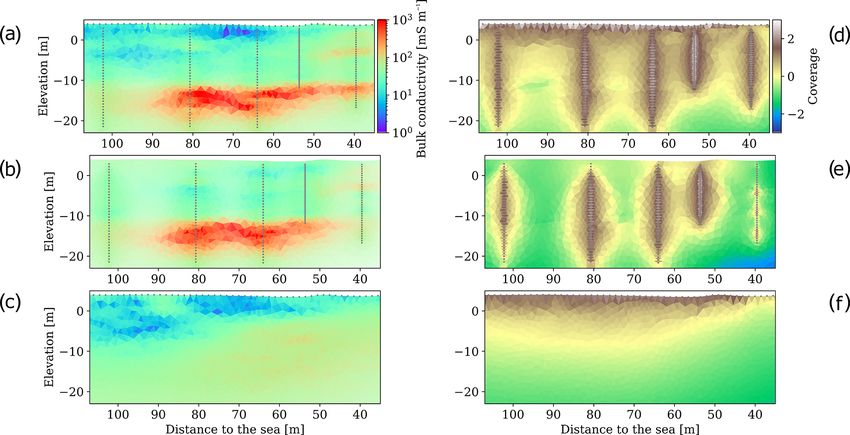
deep piezometers that do not contain any electrodes. ILs from ter zone than the complete CHERT model. Studies trying to
May 2015 (light blue), before the beginning of the CHERT link hydrological and geophysical models in coastal aquifers
experiment, are available for all piezometers. They are com- (Huizer et al., 2017; Beaujean et al., 2014; Nguyen et al.,
pared with the CHERT conductivity model from July 2015 2009) have encountered difficulties using surface ERT-based
(dark blue). In Fig. 12c, an IL from July 2016 in nest N3 models due to insufficient resolution at the depth of interest.
is compared with CHERT conductivity model from the same This lack of resolution causes the underestimation of water
month. In Fig. 12b, an IL from October 2017 in nest N4, con- EC, and thus of water salinity. The differences in the models
ducted 2 weeks after the end of the CHERT experiment, is shown in Fig. 4a suggest that surface ERT is not able to cor-
displayed with the CHERT conductivity model from Septem- rectly capture the conductivity contrasts in the subsurface.
ber 2017 of nest N3. The CHERT conductivity model can be This finding is confirmed by the validation of the CHERT
well correlated with the IL from all piezometers. There are bulk EC models with induction logs (Fig. 12).
differences in the magnitudes of the bulk EC, but both meth-
ods agree on the location of the transition zone, from −10 to 6.2 Reference model: link between bulk EC and
−12 m a.s.l. geological conceptual model
The complete CHERT produces a quite clear picture of the
link between the bulk EC model and the stratigraphic units.
Hydrol. Earth Syst. Sci., 24, 2121–2139, 2020 www.hydrol-earth-syst-sci.net/24/2121/2020/A. Palacios et al.: Time-lapse cross-hole electrical resistivity tomography 2133 Figure 12. Comparison of bulk electrical conductivity models obtained from induction logs and CHERT along piezometers in nests N2 (a), N4 (b), N3 (c) and N1 (d). The CHERT logs were extracted from the CHERT bulk EC models along the boreholes. We can explain the presence of two saline bodies with the and N225 is related to the continuity of the crystalline for- presence of a continuous semiconfining layer, and the exis- mation. Loss of resolution below PP20 and PP15 does not tence of up to three different aquifer layers. This is relevant allow us to infer anything about the presence of weathered by itself because it was unexpected. The only geologic fea- granite towards the sea. From the available data, we conclude ture is a relatively minor but apparently continuous silt layer, that the decrease in bulk EC observed in the images has two which we originally discarded as relevant. Bulk EC imag- causes: first, an important change in lithology from gravel to ing suggests that this layer may play an important role. The weathered granite; and, second, a decrease in water EC ob- transition zone is not located at the depth of the silt layer. served in the water samples from N125, with respect to the This silt layer is the one separating the unconfined from the water sample from N120 (Fig. 10). The water EC values from semiconfined aquifer. It is not, however, separating the fresh- N125 samples suggest that pore water is a mixture of fresh- water from the saltwater. The saltwater intrusion zone begins and saltwater. The granite is, most likely, not an impervious 2 to 3 m below the silt layer, thus suggesting that a significant boundary for mixing processes, but merely another source flux of freshwater occurs below this layer. This result is con- of heterogeneity in the system. The existence of freshwater sistent with sandbox experiments of Castro-Alcalá (2019), from bottom layers of the model is yet to be explored, but who found that relatively minor heterogeneities may cause it is consistent with the findings of Dewandel et al. (2006), the saltwater wedge to split. who described frequent highly transmissive zones at the base In addition, CHERT allowed us to improve the visual- of the weathered granite in numerous sites around the globe. ization of the SWI in comparison to traditional hydrology The conductive anomalies fade while moving away from monitoring methods. Indeed, using traditional methods the the sea. Above −10 m a.s.l., the small conductive anomaly silt layer would have been completely discarded as relevant, stops before PP15, and is no longer present around N325. but the CHERT made possible the visualization of a non- Below −10 m a.s.l., the conductive anomaly is present un- monotonic salinity profile that confirms the importance of the til N325, but is weaker around N225. Due to the distance heterogeneity. Specifically, salinity profiles in fully screened between piezometers N225 and N325, the sensitivity of the boreholes (such as PP20) are always monotonic (EC in- CHERT in this panel is lower than for the rest of the borehole creases with depth) and rarely reach seawater salinity. Our pairs and the decrease in the bulk EC conductivity may be imaging points out that actual salinity is non-monotonic and related to it. Nevertheless, this diminishing trend in the bulk leads to the suggestion that it is the flow of buoyant freshwa- EC reference model coincides with water EC values from ter within the borehole what explains both the observed step- piezometer N320 being slightly higher than water EC from wise increase in traditional salinity profiles and the fact that piezometer N220. We identify a vertical mixing zone, but salinity is below that of seawater. The process is described also a lateral mixing zone between nests N3 and N2. by Folch et al. (2020) and by Martínez-Pérez et al. (2018), In summary, by comparing the CHERT bulk EC model, but visualization is only possible by ERT (and specifically water EC measurements and the site stratigraphic columns, CHERT) or electromagnetic methods (e.g., induction logs). we are able to highlight several features. (1) The resistive Weathered granite was found in the cores at the bottom anomaly observed at the top is certainly related to partial wa- of N1, below −17 m a.s.l. At this depth, the magnitude of ter saturation. (2) The seemingly continuous silt layer found the CHERT bulk EC model decreases. We can, thus, infer at −9 m a.s.l. in boreholes N225, N325 and N125 does not that the decrease in bulk EC at the base of piezometers N325 represent a freshwater–seawater boundary. The freshwater– www.hydrol-earth-syst-sci.net/24/2121/2020/ Hydrol. Earth Syst. Sci., 24, 2121–2139, 2020
2134                                               A. Palacios et al.: Time-lapse cross-hole electrical resistivity tomography

seawater boundary appears 2 to 3 m below, which implies            6.4     Time-lapse study: short-term effects
that the silt layer is a semiconfining layer and freshwater dis-
charges below. (3) There are not one but two saline bodies,        6.4.1    The heavy rain: a freshwater event
one in each aquifer. The lower one is a traditional one, but the
upper one is more complex and will be discussed in Sect. 6.4.      A 220 mm – a third of the region’s average annual precipita-
(4) The conductivity value of the most conductive anomaly          tion – rainfall event lasting less than a day occurred on 12 Oc-
below −10 m a.s.l., interpreted as seawater-bearing forma-         tober 2016. It was a catastrophic event that created human
tions, decreases at the top of the weathered granite. This de-     and material losses due to flooding. The Argentona stream is
crease in bulk EC is explained by the reduction of water EC,       an ephemeral stream that carries water a few days each year
and by a reduction in bulk EC due to the larger electrical         during monsoon-like rains, typically between September and
formation factor of the granite. (5) CHERT bulk EC models          December. A rainfall of this magnitude floods the Argentona
show the location of a vertical transition zone, and also the      stream, and the entire experimental site.
extent of a lateral transition zone.                                  Do the CHERT images capture the effect of the heavy rain
                                                                   in the coastal aquifer? Figure 8a displays the difference in
6.3     Time-lapse study: long-term effects                        conductivity obtained by the tomography from 11 d before
                                                                   the rain and 9 d after the rain. The bulk EC ratio image re-
                                                                   veals a decrease in the bulk EC in both upper and lower
6.3.1    Seasonality: the natural dynamics
                                                                   aquifers. In October 2016, according to Fig. 7, the increase
                                                                   in bulk EC that was taking place was interrupted after this
The time evolution of the average bulk EC displayed in Fig. 7      heavy rainfall.
shows that there are months with a decrease in bulk EC con-           To understand the change in bulk EC, we must think
ductivity and months with an increase in bulk EC conduc-           in terms of water masses. When an important precipitation
tivity. These months are correlated with rainy and dry peri-       event occurs, freshwater flows through rivers and streams
ods, and also with the occurrence of storm surges. During          towards the sea. Inland, some freshwater infiltrates into the
summer and beginning of autumn, the conductivity increases         subsurface, pushing in situ water masses down and to the
slowly until the rain period starts; in autumn, during heavy       sides. The displacement of “old water” creates space for the
rains, conductivity decreases; during winter months, conduc-       newly infiltrating fresh rainwater, and this movement en-
tivity increases due to sea storms; in spring, conductivity de-    hances mixing processes. Offshore, surface and submarine
creases, and it reaches its lowest point before the dry sum-       groundwater discharge is occurring at the same time. The
mer period begins again. In the deeper areas where seawater        observed change in bulk EC is most likely the result of the
is already in place, average bulk EC does not show important       mixture of old saltwater with rainwater in the aquifer, which
variations.                                                        creates a new water, that is still saline but less so than before
                                                                   the rain event. However, despite the rainfall magnitude, EC
6.3.2    The drought: long-term salinization                       changes were neither dramatic nor long lasting.
                                                                      The effect of the heavy rain that lasted only a few hours
The time-lapse ratio image from September 2017 (Fig. 6l),          supports what was said in the drought section about this rain
the average bulk EC at −12.5 m a.s.l. (Fig. 7) and the water       not being representative of the region’s precipitation. One
EC measurements in the transition zone (Fig. 10) indicate          sudden episode, even of this magnitude, is not enough to
a clear increase in bulk EC in the lower aquifer since the         make a significant difference in the seawater intrusion pat-
beginning of the experiment.                                       tern and in the aquifer’s long-term salinization.
   We conjecture that this increase in water salinity is linked
to the drought that started in 2015 and had not yet ended          6.4.2    The storm: a saltwater event
by November 2017. In recent years, drought occurs every 8
to 10 years and lasts a few years. This is visible in Fig. 11      From July 2015 to October 2016, CHERT experiments had
in the years 2006–2007 and 2015–2016–2017. The effect of           conveyed that the most conductive anomaly was concen-
the decrease in freshwater recharge by rainfall is observed        trated below the silt layer, but another strong conductive body
in the experimental results, in the form of salinization of the    appeared between nest N3 and borehole PP20 early in 2017.
aquifers at a distance of 100 m from the coastline. This re-          The traditional SWI paradigm (Abarca et al., 2007; Henry,
sult is corroborated by water EC from water samples taken          1964) suggests that it is the freshwater head that drives the
at the piezometers. The overall increase in bulk EC is at-         seawater–freshwater interface movement. When heads rise,
tributed to an overall increase in water EC. While this is not     the interface moves down and seawards because freshwater
surprising, what may come as a surprise is the relatively slow     pushes saltwater seaward. When the groundwater table falls,
response of salinization of SWI to weather fluctuations. No        the opposite occurs, and the seawater interface moves up and
steady regime has been reached after 3 years and salinization      inland. The work by Michael et al. (2005) explains how other
continues.                                                         mechanisms, besides seasonal exchanges, can promote sea-

Hydrol. Earth Syst. Sci., 24, 2121–2139, 2020                                     www.hydrol-earth-syst-sci.net/24/2121/2020/
You can also read