MONITORING SURFACE DEFORMATION OF DEEP SALT MINING IN VAUVERT (FRANCE), COMBINING INSAR AND LEVELING DATA FOR MULTI-SOURCE INVERSION - SOLID EARTH
←
→
Page content transcription
If your browser does not render page correctly, please read the page content below
Solid Earth, 12, 15–34, 2021
https://doi.org/10.5194/se-12-15-2021
© Author(s) 2021. This work is distributed under
the Creative Commons Attribution 4.0 License.

Monitoring surface deformation of deep salt mining in Vauvert
(France), combining InSAR and leveling data
for multi-source inversion
Séverine Liora Furst1 , Samuel Doucet2 , Philippe Vernant3 , Cédric Champollion3 , and Jean-Louis Carme2
1 Univ.Grenoble Alpes, Univ. Savoie Mont-Blanc, CNRS, IRD, IFSTTAR, ISTerre, 38000 Grenoble, France
2 Fugro France, 115 Avenue de la Capelado, 34160 Castries, France
3 Géosciences Montpellier, Université de Montpellier, CNRS UMR-5243, 34095 Montpellier, France

Correspondence: Séverine Liora Furst (severine.furst@univ-smb.fr)

Received: 6 May 2020 – Discussion started: 19 June 2020
Revised: 23 November 2020 – Accepted: 24 November 2020 – Published: 12 January 2021

Abstract. The salt mining industrial exploitation located in     two behaviors of the salt layer: a major collapse of the salt
Vauvert (France) has been injecting water at high pressure       layer beneath the extracting wells and a salt flow from the
into wells to dissolve salt layers at depth. The extracted       deepest and most external zones towards the center of the
brine has been used in the chemical industry for more than       exploitation.
30 years, inducing a subsidence of the surface. Yearly level-
ing surveys have monitored the deformation since 1996. This
dataset is supplemented by synthetic aperture radar (SAR)
images, and since 2015, global navigation satellite system       1   Introduction
(GNSS) data have also continuously measured the deforma-
tion. New wells are regularly drilled to carry on with the ex-   Rock salt (halite) is a sedimentary rock formed by the evap-
ploitation of the salt layer, maintaining the subsidence. We     oration of seawater under specific conditions at different ge-
make use of this careful monitoring by inverting the geode-      ological times. Halite deposits are located underground or
tic data to constrain a model of deformation. As InSAR and       inside mountains, though some can also be found on the sur-
leveling are characterized by different strengths (spatial and   face in arid regions. They mainly contain crystals of sodium
temporal coverage for InSAR, accuracy for leveling) and          chlorite (NaCl) but can also include impurities such as clay,
weaknesses (various biases for InSAR, notably atmospheric,       anhydrite, or calcite. The distribution of salt deposits world-
very limited spatial and temporal coverage for leveling), we     wide is very localized, spread over areas ranging from a few
choose to combine SAR images with leveling data, to pro-         up to several hundred square kilometers. In Europe, countries
duce a 3-D velocity field of the deformation. To do so, we de-   such as Germany, Denmark, and the Netherlands have a large
velop a two-step methodology which consists first of estimat-    amount of salt (Gillhaus and Horvath, 2008). The buried lay-
ing the 3-D velocity from images in ascending and descend-       ers of rock salt can be dissolved by injecting water during
ing acquisition of Sentinel 1 between 2015 and 2017 and sec-     the so-called solution mining process. This process is used
ond of applying a weighted regression kriging to improve         to extract salt in the form of brine (for the chemical indus-
the vertical component of the velocity in the areas where        try). More commonly, solution mining aims at creating salt
leveling data are available. GNSS data are used to control       caverns for the storage of fossil fuels such as natural gas, oil,
the resulting velocity field. We design four analytical models   and petroleum products (refined fuels, liquefied gas) but also
of increasing complexity. We invert the combined geodetic        for the storage of hydrogen and compressed air (Donadei and
dataset to estimate the parameters of each model. The op-        Schneider, 2016).
timal model is made of 21 planes of dislocation with fixed          The difference between geostatic pressure and brine (or
position and geometry. The results of the inversion highlight    hydrocarbons) at cavern depth produces a change in stress

Published by Copernicus Publications on behalf of the European Geosciences Union.
16                                         S. L. Furst et al.: Monitoring surface deformation of deep salt mining in Vauvert

equilibrium that leads to elastic and visco-elastic deforma-        on the source at different time (Peltier et al., 2017). Sec-
tion of the surrounding medium (Bérest and Brouard, 2003;           ond, combining data of different temporal and spatial sam-
Bérest et al., 2006, 2012). The instantaneous (i.e., elastic)       pling rates can be done using methods of interpolation such
subsidence is due to the change in stress because of the ex-        as Gaussian process regression (kriging). These methods as-
cavation. The latter is relatively small (up to a few centime-      sume a constant deformation rate over the observed period
ters) for most salt and potash mines (Van Sambeek, 1993).           but also that the data sampling is statistically representa-
Furthermore, a time-dependent subsidence also occurs, due           tive (spatially and temporally) of the area of interest. For in-
to salt creep related to caverns opening. This long-term sub-       stance, Fuhrmann et al. (2015) developed a methodology to
sidence continues until the cavern volume vanishes, reach-          calculate and combine linear velocity rates from InSAR, lev-
ing large deformation (1 m or more) over tens or hundreds of        eling, and GNSS data measured in the Upper Rhine graben.
years (Van Sambeek, 1993). These deferred dynamic surface           InSAR, GNSS, and leveling velocities are interpolated in-
deformations may result in damage to infrastructures (e.g.,         dependently by ordinary kriging. Finally, these interpolated
pipelines, roads, buildings, railways) in the vicinity of the       datasets are merged by a least squares adjustment enabling
exploitation. Therefore, to mitigate these potential effects,       the estimate of the north, east, and vertical components of
long-term monitoring of the mining activities is usually man-       the velocity field. Similarly, Lu et al. (2015) analyze lev-
dated by governments. In this study, we focus on the par-           eling, permanent scatterers (PSs), and cross (between both
ticular monitoring of the deformation induced by rock salt          datasets) variograms over the Choushui River fluvial plain
mining in Vauvert (southern France) using geodetic instru-          in Taiwan. However, these methods are not suitable for the
ments and techniques. The extraction is performed in some           current study. Indeed, the interpolation methods (kriging and
of the world’s deepest boreholes in salt reservoirs. The sub-       co-kriging) implicitly assume that the sample is statistically
sidence has been monitored since 1996 using (1) leveling            representative (spatially and temporally) of the deformation
survey (IGN, Institut Géographique National) and (2) SAR            field. InSAR kriging works for most cases where the den-
(synthetic aperture radar) images acquired by various satel-        sity of points allows the interpretation of surface displace-
lite missions (ERS, ENVISAT, SENTINEL). With no further             ments. When several measurement techniques (GPS, level-
processing, only 1-D displacements (along the line of sight         ing, tacheometry, or inclinometry) are statistically represen-
of the satellite or the vertical component for leveling) can        tative of the deformation (spatially and temporally), the co-
be described. A previous study from Raucoules et al. (2003)         kriging method can be implemented. In this study, leveling
has identified an 8 km diameter subsidence bowl centered on         lines measure the vertical displacement and complement In-
the eastern part of the exploitation. They suggest a maximum        SAR data. We implement a methodology to estimate the 3-D
subsidence rate of 22 mm yr−1 based on the differential SAR         velocity field from the combination of InSAR and leveling
interferometry (DInSAR) technique applied to ERS-1 and              data. This 3-D velocity field provides a unique dataset reveal-
ERS-2 images from 1993 to 1999. Nevertheless, one can pos-          ing significant horizontal velocities. Considering the small
tulate that the surface deformation induced by the salt extrac-     number and the late installation of cGNSS stations (only par-
tion should include 3-D displacements rates, including hori-        tially matching the InSAR period), the resulting 3-D veloci-
zontal displacements either due to the salt flow or to the cen-     ties are not consistent in space and time. Therefore, they were
tripetal displacement associated with the subsidence. Hence,        not used to constrain the InSAR-based velocity field but only
four continuous global navigation satellite system (cGNSS)          to control the accuracy of the final velocity field in a first
stations were installed in 2015 (one station) and 2016 (three       approximation.
stations) to measure the local 3-D surface velocities.                 From the combined velocity field, models of the salt layer
   Along with spatially dense InSAR and leveling data, a            (e.g., analytical, numerical, or geomechanical) can be de-
complete description of the 3-D surface displacement rates          rived in order to improve the brine productivity and to pre-
can be assessed by combining the geodetic datasets. Indeed,         dict the evolution of subsidence. A software has already been
all three geodetic techniques measuring the subsidence in           developed for the Solution Mining Research Institute to eval-
Vauvert are complementary regarding their spatial and tem-          uate and predict surface subsidence over underground open-
poral attributes. The combination of deformation data mea-          ings (Van Sambeek, 1993). Although this model accounts for
sured according to different geometries is not trivial. The         three-dimensional geometry, the distribution over time of the
displacement values are indeed projected along the line of          openings, and salt creep, it does not include the surface data,
sight of the satellite for InSAR, along the vertical for level-     such as displacements or velocities. The model is used to
ing, and in 3-D for GNSS. Different combination techniques          simulate ground subsidence above solution-mined caverns or
have already been tested at different stages of data process-       dry mines and not to infer source parameters. Instead, geode-
ing: first, different satellite acquisition geometries (e.g., as-   tic data measured in Vauvert can be inverted to model deep
cending, descending, and ascending of parallel orbit) can be        sources of strain similarly to model sources resulting from
used to estimate the three components of the displacement           magmatic activities (e.g., Peltier et al., 2007; Camacho et al.,
(Wright et al., 2004). This implies that interferograms may         2011; Galgana et al., 2014), CO2 injection (e.g., Vasco et al.,
cover slightly different time periods including information         2008), stimulated reservoirs (e.g., Astakhov et al., 2012),

Solid Earth, 12, 15–34, 2021                                                              https://doi.org/10.5194/se-12-15-2021
S. L. Furst et al.: Monitoring surface deformation of deep salt mining in Vauvert                                              17

or gas reservoir compartmentalization (e.g., Fokker et al.,      generally found between 900 and 4900 m at depth (Fig. 1;
2012). In order to find the optimal model explaining the         Valette and Benedicto, 1995):
3-D velocity field, we consider four analytical models of
different configurations and increasing complexity: a single       1. the clay series brings together two sub-series – the “gray
point source of varying position and volume variation (Mogi,          series” (2000 m thick of deposit of clay, sand, limestone,
1958), a 2-D plane of dislocation (Okada, 1992), and two col-         marl, conglomerate, and lignite) and the “red series”
lections of 21 and 28 planes of dislocation (Okada, 1992)             (200 m of clay and gypsiferous marls with several in-
with fixed position, depth, orientation, and geometry. The            tervals of marl and sand from palustrine environment);
point source implies a simple pressurized source inducing
symmetrical vertical displacements of the surface. The hor-        2. The saliferous series (900 m thick) with four formations
izontal displacements modeled by the point source are in-             – the infra-saliferous, the lower saliferous, the interme-
duced by the centripetal displacement associated with the             diate marl, and the upper saliferous formations; these
subsidence. Contrary to the pressurized source, planar dis-           formations lie between 1500 and 3000 m deep and are
location allows for shear motion in addition to tensile motion        affected by normal faults and two thrust surfaces, i.e.,
of the plane and can therefore capture more complex pro-              decollements D1 and D2 (Fig. 1); the salt layers dip at
cesses such as salt flow. Besides, such models are also more          30 ± 5◦ ;
representative of deep salt layers. The inversion of the 3-D
                                                                   3. The marine clay series range from 800 to 1500 m thick
velocity field allows us to constrain models of the salt layer
                                                                      and correspond to three sequences of Aquitanian de-
and to give a hypothesis for the origin of the horizontal dis-
                                                                      posits, mainly composed of clay with intervals of lime-
placements.
                                                                      stones, sandstones, or layers of dolomite.
   In our study, we aim at characterizing the deformation of
salt reservoir using Sentinel-1 images, leveling lines, and      During the Miocene crustal spreading, syn-rift sediments
GNSS data. We propose a two-step methodology to com-             were covered by transgressive Burdigalian marine sediments
bine geodetic data measuring the bowl of subsidence induced      and coastal molasses before being uplifted and eroded dur-
by the salt extraction in Vauvert (Doucet, 2018). In the first   ing the Messinian event (Valette and Benedicto, 1995). The
step, we estimate the three components of the subsidence ob-     whole formation was finally overlaid by one last stage of sed-
served in Vauvert from InSAR data. In a second step, we use      imentation occurring during the Pliocene.
a regression-kriging technique, to constrain the vertical com-
ponent of the displacement using leveling data. This latter is   2.2   Salt extraction
then inverted using a gradient-based method to characterize
the parameters of each models and to define the best model of    The deep salt deposit of Vauvert was discovered dur-
the salt layer regarding the geodetic dataset. Results are in-   ing the 1952–1962 oil survey conducted by ELF (Valette,
terpreted and discussed taking into account production data      1991). Since 1972, the company KemOne (previously ELF
from the operator company and geological and geophysical         ATOCHEM-Saline de Vauvert) has been extracting the salt
complementary information.                                       from deep caverns (1500–3000 m) in the form of a solution
                                                                 saturated in salt, i.e., the brine. The brine is then carried out
                                                                 to Fos-sur-Mer (70 km southeast of Vauvert) to be used in
                                                                 the chemical industry producing chlorine and caustic soda.
2     Mining the deep rock salt deposit of Vauvert               The brine is recovered using two or three wells (doublets or
                                                                 triplets) hydraulically connected in the salt layer by initial
2.1    Geological setting                                        or induced fracturing of the medium. Among the currently
                                                                 drilled wells (about 47), only 12 are still extracting brine,
The salt deposit of Vauvert is located on the NW margin          two are being vented (to release overpressure at the well head
of the on-shore half graben of the extensional Camargue          due to salt creeping), and the other ones are sealed. For the
basin in southern France. This graben results from the Oligo-    active sets, water is injected into one well at a pressure of
Aquitanian rifting of the margin during the Mediterranean        9.5 MPa, while the second extracts the brine at 0.2 MPa. The
Sea expansion (Séranne et al., 1995). This extensional phase     underground circulation of fluid is allowed by the induced
lasts from 30 to 15 Ma and affects the rim of the Alpine belt    fracturing created to connect the wells. Once the salt con-
(Pyrenees, Languedoc, Gulf of Lion, Camargue, Valentinois,       centration in the brine reaches a minimum threshold (the ex-
Bresse, Rhine plain). The NE–SW-oriented basins are con-         tracted water does not contain enough salt to be exploited),
trolled by the SE-dipping Nîmes normal fault (Fig. 1). Ca-       doublets are abandoned and sealed. This implies an increase
margue basin contains up to 4000 m of syn-rift sediments         in pressure from the bottom to the top of the wells, due to
which overlay a substratum of carbonates from the Lower          salt creeping. For security reasons, the pressure needs to be
Cretaceous (130 Ma). The rapid Oligo-Aquitanian sedimen-         released by opening the wells, allowing brine to flow and salt
tation formed a succession of continental to lagoonal series     to creep until lithostatic equilibrium. In 2019, up to 1 × 10⁶ t

https://doi.org/10.5194/se-12-15-2021                                                            Solid Earth, 12, 15–34, 2021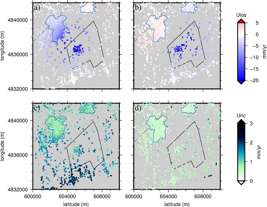
18                                          S. L. Furst et al.: Monitoring surface deformation of deep salt mining in Vauvert

Figure 1. Geological structural scheme of area under study crossing the numbered wells (Derrick symbols at the surface, pf is for Pierrefeu
well) at Vauvert (from Valette and Benedicto, 1995). D1 and D2 represent the two decollements (thrust fault) affecting the salt layers.

of brine were extracted from about four active doublets (plus           3.2   Leveling surveys
two as backup doublets).
                                                                        The height differences between two points of the network
                                                                        were determined by direct geodetic leveling (double run) car-
3     Geodetic dataset                                                  ried out using an electronic level LEICA WILD NA3003,
                                                                        on a round trip pattern. This instrument has an accuracy of
3.1    A wide network                                                   0.1 mm, and the standard deviation of measurements for 1 km
                                                                        of round-trip leveling is 0.4 mm (manufacturer data). IGN
The monitoring of subsidence above salt extraction in Vau-
                                                                        has conducted the processing using the Geolab least squares
vert has been performed since 1996 by IGN using level-
                                                                        adjustment program (version 2001.9.20.0). This type of tool
ing surveys along with a collection of InSAR data acquired
                                                                        makes it possible to provide for each of the points an ele-
by various satellite missions (ERS, ENVISAT, SENTINEL;
                                                                        vation as well as an indicator of the accuracy of the result.
Fig. 2a). Raucoules et al. (2003) first characterized the sub-
                                                                        The accuracy is estimated from the observations and not only
sidence using from ERS-1 and ERS-2 images. Only vertical
                                                                        from manufacturer nominal features. The mean data uncer-
velocity could be estimated, leading to a maximum subsi-
                                                                        tainties from the 2019 survey reaches 1.34 mm. Figure 3 il-
dence rate of 22 mm yr−1 . A permanent GNSS station was
                                                                        lustrates the leveling measurements performed between 1996
installed in November 2015 followed in October 2016 by
                                                                        and 2018 along the profile A–B in Fig. 2b. These surveys
three new permanent stations. Figure 2a represents the tem-
                                                                        started in 1996 with 39 leveling benchmarks; new ones (al-
poral coverage of all geodetic techniques employed to mon-
                                                                        most 100) were added progressively to densify the network
itor the site. In this study, we only use Sentinel images be-
                                                                        and some needed to be replaced (destruction, shift, insta-
cause of their general features, including medium resolu-
                                                                        bility of a benchmark). Since 2006, about 137 benchmarks
tion, high revisit time (6 d), intermediate acquisition band
                                                                        have been measured yearly (except in 2013 and 2015). The
(C-band), and easily accessible data. Hence, we derive an
                                                                        velocity associated with the subsidence of the marker high-
annual deformation velocity from InSAR analysis (Sentinel-
                                                                        lighted by the red rectangle in Fig. 3 is estimated by the ratio
1a/b images) and leveling surveys measuring between 2015
                                                                        of the vertical displacement over the time interval between
to 2017 and permanent GPS data (2015–2019). Figure 2b
                                                                        two measurements (i.e., 1 or 2 years). The vertical velocity
shows the spatial coverage of leveling surveys and GPS net-
                                                                        is variable in time (Fig. 3b), with a strong increase in the
works used in this study.
                                                                        subsidence rate between 2002 and 2003; since then the sub-
                                                                        sidence rate has been relatively steady around 26 mm yr−1 in
                                                                        the center of the subsidence area (red line in Fig. 3b).

Solid Earth, 12, 15–34, 2021                                                                   https://doi.org/10.5194/se-12-15-2021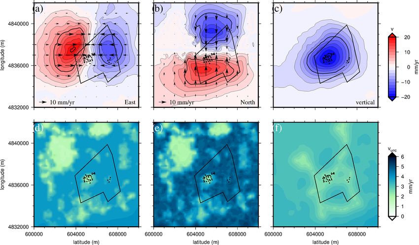
S. L. Furst et al.: Monitoring surface deformation of deep salt mining in Vauvert                                                   19

                                                                        and an incidence angle of 32.93◦ , while descending geome-
                                                                        try is defined by a flight direction with respect to the north
                                                                        of 256.01◦ and an incidence angle of 36.98◦ . We develop
                                                                        a PS–InSAR processing chain based on existing algorithms
                                                                        (e.g., SNAP, StaMPS). The preparation of single-look com-
                                                                        plex (SLC) images and the creation of the interferograms are
                                                                        carried out with the software SNAP from the European Space
                                                                        Agency (ESA). Precise orbits provided by ESA (DORIS) are
                                                                        applied to finely process the geometric positioning of the im-
                                                                        age portions (bursts). Master image are chosen so that the
                                                                        time and the perpendicular baseline are optimized: images
                                                                        of 26 November 2016 for the descending geometry and 27
                                                                        November 2016 for the ascending geometry. The two SLC
                                                                        images (master image and slave image) of the same subdo-
                                                                        main are co-registered using the orbits of the two products
                                                                        and the 90 m resolution digital terrain model, Shuttle Radar
                                                                        Topography Mission (SRTM) (Farr and Kobrick, 2000; Farr
                                                                        et al., 2007). With known satellite orbits, a correction of the
                                                                        effect of the Earth’s curvature on the phase is applied. The
                                                                        geodetic reference system is defined by the satellite orbit
                                                                        reference system (WGS84, the reference system used by all
                                                                        space SAR systems). The topographic phase is removed from
                                                                        the interferogram using SRTM. In addition, the information
                                                                        about the altitude is available for each PS.
Figure 2. (a) Temporal coverage of geodetic networks monitoring
                                                                           Once the interferograms are created under SNAP, they are
the site. (b) Spatial coverage of GNSS and leveling network of the
salt exploitation in Vauvert. Well heads are represented by red cir-
                                                                        imported and processed with StaMPS processing software
cles, permanent GNSS is represented by yellow inverted triangles,       (Hooper et al., 2004). The pixels are selected according to
and leveling benchmarks are identified by blue crosses. The red line    an amplitude dispersion criterion, and a maximum propor-
indicates the profile A–B for leveling data represented in Fig. 3a.     tion of “false” PSs is set to 20 %. Digital elevation model
The blue areas represent the extent of Vauvert and Beauvoisin cities,   (DEM), master atmosphere, orbit, and look angle error are
while the black line defines the extent of the KemOne company. The      estimated and removed. Finally, the fringes of the resulting
background map is extracted from IGN SCAN 1 : 25 000 (© IGN).           phase are unwrapped (Fig. 4a and b for ascending and de-
                                                                        scending geometries, respectively). From the unwrapped in-
                                                                        terferograms, we have relative displacements in time associ-
3.3   InSAR data                                                        ated with each PS. Then, by applying a linear regression on
                                                                        relative displacements from each PS, we get position time se-
Radar images from Sentinel constellation imaging satellites             ries. A previous study (Raucoules et al., 2003) and leveling
(Sentinel-1a and Sentinel-1b) are recorded on the C-band                measurements have shown that velocity can be considered
frequency (similarly to Envisat) and present a short tempo-             constant with time. So, using a linear regression over the 2-
ral redundancy of about 6 d, limiting the temporal decor-               year time period of this study, this leads to velocities. Asso-
relation. The perpendicular baseline between the images is              ciated uncertainties are finally obtained using the standard
very short, a few tens of meters, which also limits the spatial         deviation of PS velocities. The maximum subsidence rate
decorrelation. Sentinel constellation images have a swath of            is 24 mm yr−1 . The associated uncertainties are lower than
250 km wide and a resolution of 5 m × 20 m, in both ascend-             4.5 mm yr−1 for the ascending track and 2.9 mm yr−1 for the
ing and descending geometries. InSAR accuracy is strongly               descending track with mean values of 1.2 and 0.6 mm yr−1 ,
dependent on several factors, including SAR data and PS                 respectively (Fig. 4c and d).
availability, artificial corner reflectors, the ambiguous nature
of the observation, line-of-sight deformation measurements,             3.4   Continuous GNSS
and deformation tilt and trends (Crosetto et al., 2016). The
velocity along the line of sight can be measured with an ac-            Four permanent GNSS stations (Fig. 2) sampling at 30 s were
curacy of a few millimeters. In this study, we used 101 as-             set up, respectively, in November 2015 (VAUV station) and
cending and 66 descending images between 18 April 2015                  October 2016 (VAU1, VAU2, and VAU3 stations) to charac-
to 3 December 2017 to produce a mean displacement veloc-                terize more accurately and in three dimensions the variations
ity field and time series. Ascending geometry is character-             in the deformation and its spatial extension. The measure
ized by a flight direction with respect to the north of 103.96          of the GNSS position is a three-component value generally

https://doi.org/10.5194/se-12-15-2021                                                                  Solid Earth, 12, 15–34, 2021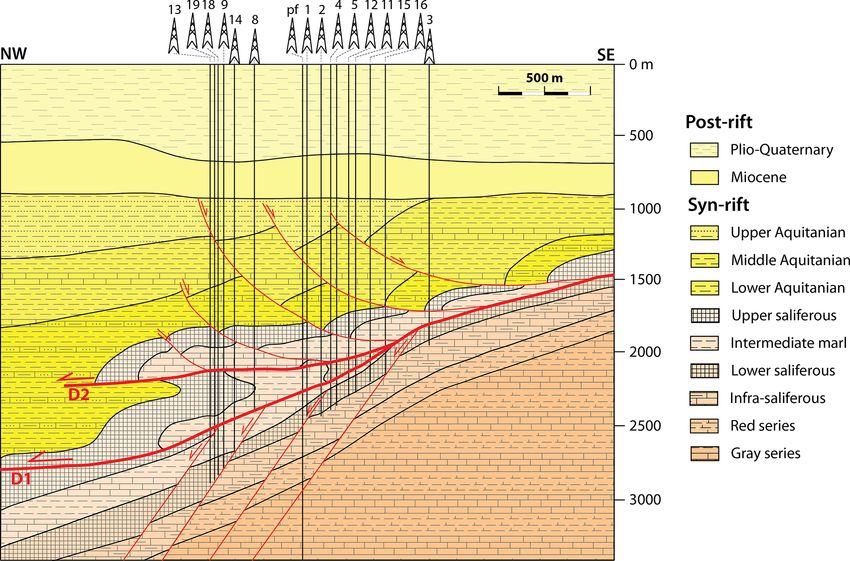
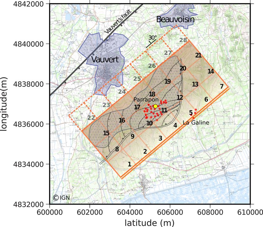
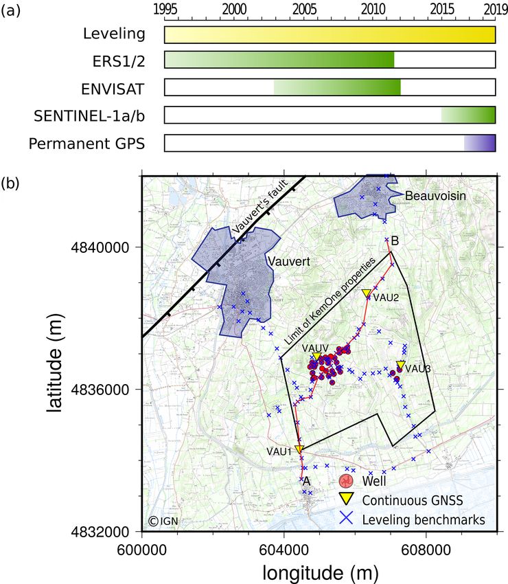
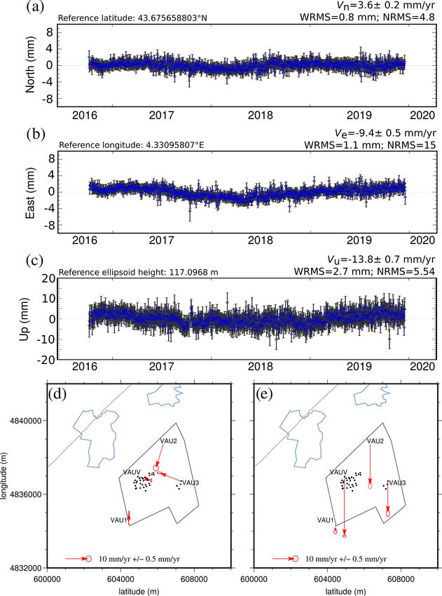
20                                            S. L. Furst et al.: Monitoring surface deformation of deep salt mining in Vauvert

Figure 3. (a) Leveling data along the A–B profile (red line in Fig. 2b) performed by IGN from 1996 to 2018 (color scale). Data are displayed
every 2 years for ease of reading. (b) Deformation velocity associated with the marker with the largest subsidence (red rectangle in a). The
velocity is given for each year, using the same color scale as in (a). The red dashed line represents the mean velocity of vertical displacement
observed from 2004 to 2018.

Figure 4. Mean velocity in LOS direction in (a) ascending and (b) descending interferograms over the area of interest and their associated
uncertainties (c) and (d), respectively. Ascending geometry is characterized by a flight direction with respect to the north of 103.96◦ and
an incidence angle of 32.93◦ . Descending geometry is defined by a flight direction with respect to the north of 256.01◦ and an incidence
angle of 36.98◦ . The polygons represent the extent of Vauvert and Beauvoisin cities (blue polygons) and the KemOne company area (black
polygons; see Fig. 2b).

given with a daily accuracy of 1 mm (Hager et al., 1991) with             2006, for details). We include in the processing 26 contin-
respect to a reference frame called the International Terres-             uous stable reference stations located within a 150 km ra-
trial Reference Frame (ITRF). The processing of coordinates               dius of the Vauvert sites. These sites belong to the perma-
and velocities is done using the Gamit-Globk v10.7 software               nent RGP, RENAG (RESIF-RENAG French national Geode-
(Herring et al., 2015). We use the well-documented three-                 tic Network; RESIF – Réseau Sismologique et Géodésique
step approach and take advantage of the “realistic sigma”                 Français), or ORPHEON networks and allow us to define a
algorithm to estimate the uncertainties (see Reilinger et al.,            stable regional reference frame by minimizing the velocities

Solid Earth, 12, 15–34, 2021                                                                       https://doi.org/10.5194/se-12-15-2021
S. L. Furst et al.: Monitoring surface deformation of deep salt mining in Vauvert                                                 21

of these 26 sites. The resulting station position time series for           ciently constrained, so obvious PSs along roads (espe-
the north, east, and vertical components are free of any re-                cially crossing roads) were used to obtain latitude and
gional tectonic displacement and show only local processes.                 longitude shifts. In order to compare InSAR to level-
   Figure 5a–c plot the time series of the three components                 ing and GNSS data, we first correct the horizontal posi-
of VAU3 station (Fig. 2) from 2016 to 2019. Once the sea-                   tion of PS points using the mean value of all horizontal
sonal effects are removed, the trends are quasi-linear in time              shifts manually detected on the interferograms. Second,
for all three components. We represent the velocities of the                we adjust the reference system of interferograms using
sites near the exploitation with respect to a local stable refer-           a two-dimensional linear ramp (Lundgren et al., 2009;
ence frame in Fig. 5d and e (i.e., all the velocities outside of            Hammond et al., 2010) based on the calculation of dif-
the mapped area can be considered as equal to ∼ 0 mm yr−1 ).                ferences between velocities at 26 GNSS stations and PS
The horizontal velocities (Fig. 5d) measured at each station                data points near these stations.
show a significant displacement toward the center of the ex-
ploitation. The vertical velocity (Fig. 5e) indicates a max-         2. Sufficient measurement density. We assume that the
imum subsidence of −25.8 ± 0.2 mm yr−1 but with greater                 density of reliable permanent scatterers is sufficient for
magnitudes at the edges of the bowl (−13.8 ± 0.7 mm yr−1                the considered area in both ascending and descend-
at VAU3 and −17.9 ± 0.7 mm yr−1 at VAU2) than those pre-                ing InSAR geometry results. Besides, we consider that
viously measured (Raucoules et al., 2003).                              leveling and InSAR measurements are dense enough
                                                                        to be statistically representative of the deformation.
                                                                        Hence their distribution can be interpolated using krig-
4     Geodetic data combination                                         ing methods (ordinary and weighted regression).

4.1     Methodology                                                  3. Satellite measurement geometry. We assume that for the
                                                                        area of interest, flight directions of the satellite with re-
4.1.1    General remarks on the combination                             spect to the north (β) are symmetrical with respect to the
                                                                        north–south axis (β asc = 103.96◦ and β dsc = 256.01◦
Terrestrial (e.g., leveling, inclinometry) and satellite-based          with respect to the north, leading to identical look an-
(e.g., GNSS, InSAR) geodetic measurements are comple-                   gles for both geometries). The angles of incidence be-
mentary in terms of accuracy and spatial or temporal resolu-            tween the satellite and the permanent reflectors at the
tion, from slow ground displacement monitoring (e.g., Has-              surface are considered nearly identical in the ascending
taoglu et al., 2017) to rapid surface changes (e.g., Peltier            and descending geometry acquisition (2asc = 32.93◦
et al., 2017). Many attempts to combine these geodetic mea-             and 2dsc = 36.98◦ ). This allows us to estimate the east
surements have been described and published recently (e.g.,             component of the deformation along with a near-vertical
Catalão et al., 2009; Burdack, 2013; Lu et al., 2015), to               component.
overcome the limitations and inadequacies of the different
                                                                     4. Radial deformation. The surface deformation observed
techniques in difficult contexts, when taken separately (e.g.,
                                                                        in the area of interest shows a quasi-symmetrical bowl
Karila et al., 2013; Abidin et al., 2015; Fuhrmann et al.,
                                                                        of subsidence (Raucoules et al., 2003). We hence make
2015; Comerci and Vittori, 2019). The combination of sev-
                                                                        the assumption that this symmetry affects all compo-
eral geodetic measurement techniques aims to improve the
                                                                        nents of the displacement, leading to the estimation of
knowledge of the ground motion by overcoming or at least
                                                                        the north component with an acceptable accuracy.
mitigating each technique’s shortcomings with the other. In
this study, we propose a methodology to combine InSAR and              Although these hypotheses may be false for other cases, in
leveling data to produce a 3-D velocity field associated with       the case of Vauvert, and given the previous available informa-
the salt extraction of Vauvert (Doucet, 2018). Unlike GNSS          tion from InSAR (Raucoules et al., 2003) and leveling, they
and leveling data that are precisely constrained on the Terres-     allow us to compute the first-order three-dimensional veloc-
trial Reference Frame (TRF), InSAR is a relative measure-           ity field associated with the salt extraction. We review and
ment in space and time, with no precise datum. So, InSAR            comment on these choices in the discussion regarding the
data have to be adjusted, constrained, or tied-in to a TRF.         results of both the combination and the inversion. Figure 6
The number of GNSS stations and, mostly, the temporal cov-          represents the general algorithm of our two-step methodol-
erage of time series are not statistically representative of the    ogy to combine interferograms and leveling data involving
deformation for being appropriately incorporated in the com-        (1) a 3-D geometrical estimation and (2) a weighted regres-
bination (only one out of four stations continuously measured       sion kriging.
the deformation between 2015 and 2017). Indeed the combi-
nation is based on the following assumptions.                       4.1.2     Step 1: 3-D geometrical estimation

    1. Reference frames adjustment. Horizontal absolute po-         The first step of the approach consists of interpolating the
       sitioning, at the time of the processing, was not suffi-     ascending and descending InSAR data by ordinary kriging,

https://doi.org/10.5194/se-12-15-2021                                                                Solid Earth, 12, 15–34, 2021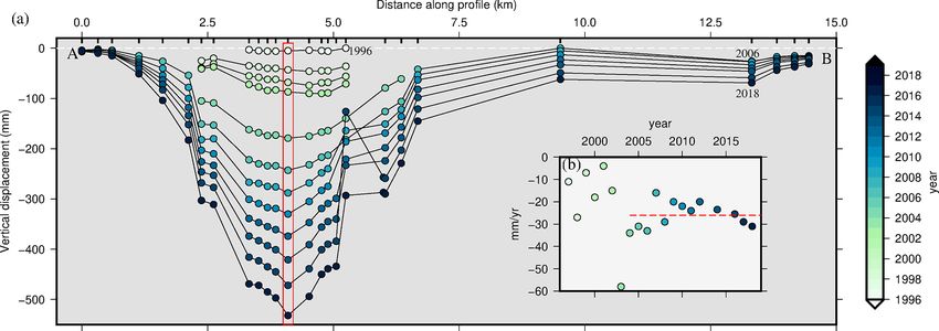
22                                           S. L. Furst et al.: Monitoring surface deformation of deep salt mining in Vauvert

Figure 5. Time series of the three components (a) north, (b) east, and (c) vertical, measured at station VAU3 from 2016 to the end of 2019.
(d) Map of horizontal velocities and well locations. (e) Vertical velocities, downward being subsidence. The polygons represent the extent of
Vauvert and Beauvoisin cities (blue) and the KemOne company area (black; see Fig. 2b).

in order to densify the spatial distribution of PS points, so            the effect of a high-density area, typically cities, where PSs
that they can be virtually colocated with leveling bench-                are more concentrated than elsewhere, notably poorly an-
marks. The kriging interpolation models the best linear un-              thropized areas where the number of data points can be low.
biased prediction of the intermediate values by a Gaussian               We use ordinary kriging to densify the spatial distribution
variogram model (driven by prior covariances). The number                of PSs (Cressie, 1988; Yamamoto, 2005; Daya and Bejari,
of data points, position, and uncertainties are considered in            2015; Ligas and Kulczycki, 2015). The associated uncertain-
the interpolation, leading to interpolated values of the data            ties are given by ordinary kriging as the weighted variance of
distribution along with uncertainties (kriging variance that             the interpolated distribution of PSs.
accounts for the data uncertainties). By applying a weighting               The velocity vPS , measured at each point on the ground,
function based on the correlation between the data and the               corresponds to the component along the radar line of sight
distance between them, the kriging method allows canceling               (LOS) of the deformation. It contains portions of all three

Solid Earth, 12, 15–34, 2021                                                                     https://doi.org/10.5194/se-12-15-2021
S. L. Furst et al.: Monitoring surface deformation of deep salt mining in Vauvert 23
assume that the horizontal component of the velocity is ra-
dial and pointing towards the center of subsidence. Using
an east–west profile crossing the center of subsidence, we
project the horizontal component of the velocity of crossed
points (i.e., pure east velocities) onto this profile to deduce
the north component. We rotate the profile around the center
of subsidence and adapt its length to the bowl size, to get the
horizontal component (including ve and vn ). When the profile
is oriented along the north–south axis, pure vn is estimated.
The 3-D components of the velocity field derived from In-
SAR can be defined as
ve = 0.9 (v dsc − v asc ), (3)
q
vn = (vh2 − ve2 ), (4)
asc dsc
vu = 0.61 (v +v ) − vn , (5)
Figure 6. Algorithm of the two-step methodology developed to
combine deformation velocities estimated from interferograms and where vh is the velocity in the horizontal plane of a point p,
leveling surveys. (1) Three-dimensional geometrical estimation is such as
performed to derive east, north, and vertical components from as-
cending and descending InSAR geometries. (2) The vertical com- π −α α
ponent and leveling data are combined using a weighted regression- vh = |vhe | + vhw , (6)
π π
kriging technique.
where α is the angle between the E–W axis and the az-
imuth of the profile relative to the center of the bowl. vhe
dimensions of the velocity, depending on the geometry of and vhw correspond to the velocities projected along the pro-
the acquisition and the angle between the vertical and the file (of zero velocity), crossing the center of subsidence. This
measured point, such as method allows us to estimate the north component from a
complex shape of subsidence bowl, considering a radial sur-
vPS = s · v, (1) face deformation. From these relations, we produce the three-
where v is the three-dimensional vector of the velocity and s dimensional velocity field associated with the extraction of
is the unit vector pointing from the ground towards the satel- salt in Vauvert.
lite. This unit vector is defined by the incidence angle (2)
4.1.3 Step 2: weighted regression kriging
and by the flight direction with respect to the north (β) asso-
ciated with each geometry of acquisition. In the second step of our combination approach, we use a
− sin 2 sin β
regression-kriging method (e.g., Hengl et al., 2007) to re-
s = − sin 2 cos β (2) fine the vertical velocity field in the areas where leveling data
− cos 2 are available. Indeed, leveling surveys provide accurate mea-
surements of the vertical velocity field but only on a finite
Using assumption 3 from Sect. 4.1.1 leads to components number of points (120). Regression kriging is a spatial pre-
of the unit vectors for ascending and descending geometries diction technique that combines a regression of the depen-
n = s n = −0.13, s v = s v = 0.82, and s e =
such as sasc dent variable (dual geometry InSAR in our case) on auxil-
dsc asc dsc asc
e
−sdsc = 0.55. Because the maximum deformation in the area iary variables (leveling data in our case, but it could also be
of interest is on the order of 10 to 20 mm yr−1 (for the GNSS if they were consistent in time) with kriging of the re-
north and vertical components), this assumption induces er- gression residuals. It is mathematically equivalent to kriging
rors ranging from 0.1 to 0.8 mm yr−1 , which are 1 order of with external drift, where auxiliary predictors (leveling) are
magnitude lower than data uncertainties. Using the compo- used directly to solve the kriging weights (Pebesma, 2006).
nents of the unit vectors for ascending and descending ge- Also, leveling benchmarks are only distributed along linear
ometries, we can deduce the relation to estimate the east and paths, making the use of co-kriging inappropriate to com-
a near-vertical component of the velocity. The near-vertical bine InSAR and leveling data on a spatial grid. Instead, re-
component vnu is used to defined the complex geometry of gression kriging uses regression on auxiliary information and
the subsidence bowl, so that its shape is given by the iso- then uses simple kriging with known mean (0) to interpolate
contour vnu = 0 and its center is determined by the junction the residuals from the regression model (Hengl et al., 2004).
of the maximum subsidence (vnu min ) and zero velocity along This method allows us to make predictions by modeling the
the east–west direction. To extract the north component we relationships between the target and one or more auxiliary
https://doi.org/10.5194/se-12-15-2021 Solid Earth, 12, 15–34, 2021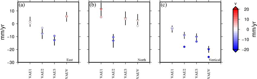
24 S. L. Furst et al.: Monitoring surface deformation of deep salt mining in Vauvert
variables (the predictor(s)) at common sampling locations. shifting accordingly). However, even though the combined
In this study, we use the generic framework developed by set and the GNSS are fairly consistent with each other, it shall
Hengl et al. (2004) for spatial prediction of the vertical ve- be emphasized that they could not perfectly match each other
locity field. We sample the vertical velocity field from InSAR due to their different time coverages of an area very sensitive
data (target data) at the leveling benchmarks’ location (aux- to the location of the extraction wells (which were shifted in
iliary data). Then, a linear regression of a target variable (vu ) time).
on predictors (leveling) is applied with a kriging of the resid-
uals of the prediction. Finally, we estimate a reliability index
at each point of the grid, taking into account the uncertain- 5 Multi-source inversion
ties of each technique and the uncertainty associated with the
interpolations. 5.1 Forward models
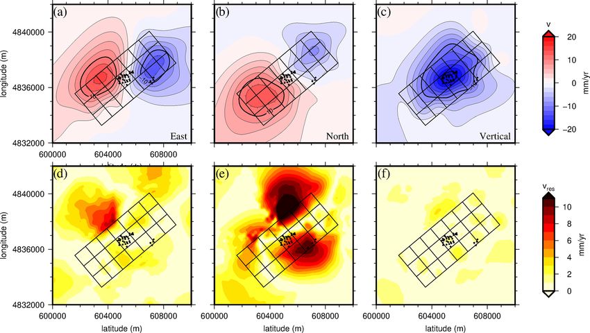
On Fig. 7a to c we represent east, north, and vertical com-
ponents of the velocity resulting from the data combination, The salt formation lies between 1500 and 3000 m deep in
along with their associated uncertainties (Fig. 7d to f). The sheet-like layers dipping at 30 ± 5◦ induced by the presence
incorporation of leveling data in the combination allowed of normal faults and two decollements D1 and D2 (Valette
refining the vertical component of the velocity measured and Benedicto, 1995; Fig. 1). Previous studies (Maisons
from dual geometry InSAR. The deformation induced by the et al., 2006; Raucoules et al., 2003, 2004) have highlighted a
salt exploitation in Vauvert is characterized by both hori- quasi-perfect axi-symmetrical bowl of subsidence in Vauvert
zontal and vertical displacements. Compared to Raucoules originating from the exploitation of this salt formation. In this
et al. (2003), the combined dataset (along with GNSS ve- study, the combined dataset (Fig. 7) shows a consistent verti-
locities) allows us to identify significant horizontal displace- cal signal but also provides horizontal displacements. Hence,
ments. East and north components of the velocity field indi- we consider four analytical models of the salt layer of in-
cate a maximum subsidence rate towards the center of the creased complexity to best explain the velocity field mea-
exploitation (Parrapon site, black dots in Fig. 7) of about sured by the geodetic dataset: a single point source, a rectan-
18 mm yr−1 (Fig. 7a and b). The maximum vertical veloc- gular plane, and two collections of 21 and 28 square planes.
ity reaches 24 mm yr−1 (Fig. 7c) and is located above the salt In the case of Vauvert’s exploitation, using elastic models al-
exploitation of Vauvert. The subsidence affects a large area lows us to model the surface displacements induced by the
in a radius of about 3 km from the center of the exploitation brine extraction but also possibly by salt creep. However salt
(black dots in Fig. 7). creep is reduced to shear on planes without any further rheo-
logical considerations.
4.2 Comparison with GNSS velocity field First, we use a simple Mogi source (Mogi, 1958) to
model the volume variations in the salt layers at depth
The combination of InSAR ascending and descending data (model 1). It considers a spherical source embedded in a
with leveling data produces a 3-D velocity field measuring semi-infinite uniform elastic body. The source is defined by
the deformation above the salt exploitation of Vauvert. The four variables: its Cartesian coordinates (xs , ys , zs ) and its
vertical velocity computed through this combination is fairly volume variation (1V ). The point source being the less rep-
similar to the one estimated by Raucoules et al. (2003). Dif- resentative model of the salt layers, we do not constrain it
ferences may notably stem from both the period of inter- with geological information and keep the four variables of
est and the incorporation of leveling data (as opposed to the source free during the inversion.
stand-alone InSAR). In Fig. 8, we compare the three com- Second, we consider a 2-D plane of dislocation (model 2)
ponents of the velocity field derived from the dual InSAR with parameters (position, depth, dimensions, dip, azimuth)
geometry–leveling combined set to their GNSS counterparts. set according to the salt layer properties for a more realis-
It shall be noted that the GNSS uncertainties are lower than tic model. The forward model uses three-dimensional, elas-
0.8 mm yr−1 , so not significant enough to be represented in tic dislocation theory in a homogeneous half space (Okada,
the figure. Even though this comparison is only indicative 1992). The source is a patch, characterized by its posi-
due to observation times not perfectly matching each other, tion, dip, azimuth, length, width, depth, and dislocation
one may notice, however, that on all four points the com- type (strike, dip, or tensile). The plane is centered on the
bined set correctly matches the GNSS in both east and north salt exploitation at a depth of −2250 m and covers the al-
(with the GNSS circles located within the uncertainty bars), lochthonous saliferous unity, up to La Galine’s boreholes
whereas there is no matching in the vertical for two points (orange rectangle in Fig. 9). The plane has a strike dip of
(VAU2 and VAUV). The latter inconsistency is all the less N 50◦ E, 30◦ NW with depths ranging from 1500 to 3000 m
surprising as VAUV is located close to the subsidence bowl (the top of the plane, at 1500 m, is identified with the dou-
center (where subsidence magnitude is changing faster) and ble orange line in Fig. 9). Most of the exploitation wells (red
VAU2 is located close to the north edge of the bowl (the sub- dots in Fig. 9) are located at the Parrapon site. La Galine’s
sidence bowl has migrated northward due to extraction wells wells are no longer active (two wells), and brine is extracted
Solid Earth, 12, 15–34, 2021 https://doi.org/10.5194/se-12-15-2021S. L. Furst et al.: Monitoring surface deformation of deep salt mining in Vauvert 25
Figure 7. The three components (east, north, and vertical) of the velocity field calculated using the two-step methodology described in this
section (a–c) and their associated uncertainties (d–f). Black arrows indicate the horizontal velocities on (a) and (b). The black dots show the
well locations. The black polygon represents the KemOne company area (see Fig. 2b).
Figure 8. Three components of the velocity from GNSS and the Dual InSAR geometry–leveling combined dataset observed at GNSS
locations (VAU1, VAU2, VAU3, VAUV; see Fig. 2). Inverted triangles represent the (a) east, (b) north, and (c) vertical components of the
velocity from the combined dataset, the vertical bars indicate the associated uncertainties, and the circles stand for the GNSS dataset.
only to release pressure. It means a very low brine production The combined velocity field suggests a more complex
during the time considered. All but the dislocation parame- source deformation and a single source may not be sufficient
ters are fixed using available geological information, such as to explain the surface subsidence. Thus, we discretize the salt
the inversion process seeking only three parameters. Hence, layer into several dislocation patches, to increase the degrees
Green’s functions describing the analytical solution for the of freedom for the sources to model the surface deformation.
surface displacements v (Okada, 1992) are linear with the The single rectangular plane is subdivided into 21 square
dislocation parameters: planes (model 3) of 1 km side. The orientation is the same for
the 21 patches and locations and depths are set accordingly
3
N X
X to the salt layer characteristics, all these parameters are fixed
v= Uji α ij , (7)
(Fig. 9). In this model, each plane has its own independent
i=1 j =1
strike-slip, dip-slip, and tensile components, such that both
where Uji is the dislocation type j (strike 1, dip 2, or tensile the rapid depletion at the vicinity of the exploiting wells and
3) associated with each plane i and α ij is three-dimensional the creeping deformation in the salt layer can be considered.
vectors between the point at the surface with the displace- We consider 63 free dislocation parameters to be retrieved by
ment v and the dislocation at depth.
https://doi.org/10.5194/se-12-15-2021 Solid Earth, 12, 15–34, 202126 S. L. Furst et al.: Monitoring surface deformation of deep salt mining in Vauvert
J = D T 6 −1 D, (8)
where 6 is the data covariance matrix associated with each
point of the dataset and T denotes the transpose of the resid-
ual vector. Through this formulation of the functional, we
consider the resolution of the measurements: for highly un-
certain data, their covariance matrix is large compared to the
data values, leading to small values of J . This functional
needs to be lower than the data uncertainties or reaches a
minimum value for the optimization to be completed. This
linear problem (Eq. 7) is solved using an optimization algo-
rithm allowing us to process problems with non-linear rela-
tions. By doing so, we can easily switch to a different for-
ward model, including more complex and realistic physics
without implementing a new optimization approach. Our op-
timization process is based on a recursive algorithm defining
Figure 9. Representations of the dislocation planes (numbering a multi-criteria global optimization, varying not only the pa-
from 1 to 28) are displayed in shaded orange modeling the salt rameters of the model but also the initial guesses (Ivorra and
layer (darker shading for deeper planes), along with the currently Mohammadi, 2007; Mohammadi and Pironneau, 2009). This
known boreholes (red dots). The decollements are represented by allows us to ensure that a given set of optimal model param-
the double line and listric faults by black lines beneath the site of eters realizes the global minimum of the functional.
salt exploitation in Vauvert (France). The allochthonous saliferous To determine the model parameter uncertainties, we im-
unity is represented by the gray dotted area. The limits of Vauvert plement the approach developed by Mohammadi (2016)
and Beauvoisin cities are represented by blue areas, and the Vauvert using backward uncertainty propagation. This approach is
normal fault is displayed using black lines (modified from Valette
based on the introduction of directional quantile-based ex-
and Benedicto, 1995). The blue polygons represent the extent of
Vauvert and Beauvoisin cities (see Fig. 2b). The background map is
treme scenarios knowing the probability density function of
extracted from IGN SCAN 1 : 25 000 (© IGN). the target data. By doing so, we avoid computing numerous
scenarios of data perturbation to generate the probability den-
sity function (PDF) of a functional J . Instead, we use the
inverting the combined dataset, fixing all other parameters of sensitivity of the functional with respect to the data and ex-
the planes (positions, orientations, dimensions). plore only the optimal region given by the optimization to
For model 4, we add a fourth row of planes (dashed orange identify two directional extreme sets of data. Two datasets
line in Fig. 9) to study whether boundary effects in model 3 v±i are obtained by perturbating observed data v i knowing
exist. This last row of planes is set at 3250 m depth (bottom of the associated data uncertainty σi along the direction given
planes is at 3500 m), and its extension at the surface reaches by residual value between optimal and observed data v ∗i − v i
the limits of Vauvert city. Similarly to model 3, only disloca- (the fractional term is equal to 1 or −1).
tion parameters are optimized, leading to 84 free parameters
to be retrieved. v ∗i − v i
v±
i = v i ± 1.65 σi (9)
kv ∗i − v i k
5.2 Inversion strategy
These two datasets are then inverted to obtain two sets of op-
For model 1, the position of the source is sought in the timal parameters, corresponding to the extreme values each
10 km × 10 km area defined by Figs. 2 and 9. Source depth parameter can take given the uncertainties on the observa-
can vary between 0 and 5000 m depth, and volume variation tions and the residuals. The maximum and minimum devia-
is investigated between 0 and −1.5 × 10⁶ m3 . For models 2 tions for the optimal parameter set are hence given by these
to 4, the dislocations parameters (strike-slip, dip-slip, and two extreme scenarios.
opening) are set free to vary between −1 and 1 m throughout
the inversion process. For the multi-source models (3 and 4), 5.3 Results of the inversion
no smoothing conditions are considered between planes. Ini-
tialized with no a priori information, a first modeled dataset is 5.3.1 Model comparison
produced which is compared to the observations. We choose
We compute the difference between the observations and the
to build the functional as the weighted Euclidian norm of the
model to obtain the residual values. These residuals are used
residual vector D between observed and modeled dataset:
with the data uncertainties to estimate how the model fits
Solid Earth, 12, 15–34, 2021 https://doi.org/10.5194/se-12-15-2021S. L. Furst et al.: Monitoring surface deformation of deep salt mining in Vauvert 27
the dataset using the normalized rms (NRMS) (McCaffrey, of −556 000 m3 corresponding to a mass of 1.21 × 10⁶ t per
2005): year of extracted salt, which slightly overestimates the real
" !#1/2 mass of salt.
N
NRMS = N −1
X
2
ri /σi2
, (10) Increasing the number of planes to 28 in the model by
i=1
adding a fourth row at greater depth does not improve
the residuals nor the fit to the horizontal components. Be-
where N is the number of observations, r is the residual, and
sides, the volume change associated with this model reaches
σ is the data uncertainty. This unitless level indicates whether
−751 000 m3 (1.6 × 10⁶ t of brine), largely overestimating
the model fits the observations with respect to data uncertain-
the real volume loss.
ties and should be close to 1. Besides, we can also compute
The geometry of 21 dislocation planes model, the resid-
the weighted rms (WRMS) from McCaffrey (2005), which
uals (NRMS and WRMS), the estimated volume loss, and
gives an estimation of the a posteriori weighted scatter in the
the agreement with the geological setting of the salt layers
fit.
" !
!#1/2 (Fig. 1) suggest that it is the best model. We hereafter de-
XN XN scribe the results of the inversion for this model.
2 2 2
WRMS = ri /σi 1/σi (11)
i=1 i=1 5.3.2 Parameters and resolution analysis
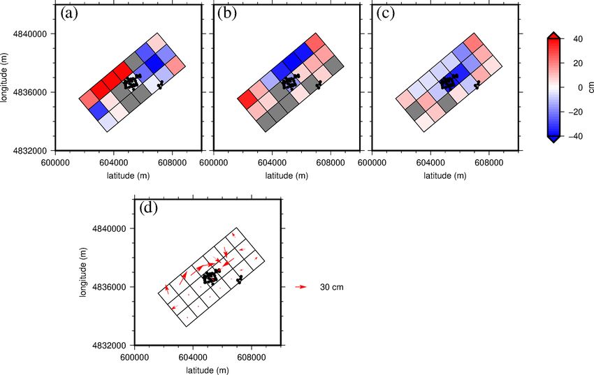
Table 1 present the residuals, NRMS and WRMS for the east,
north, and vertical components of the velocity field for each The inversion leads to a distribution of strike-slip, dip-slip,
model. The total NRMS and WRMS are also given in Ta- and tensile dislocations associated with each plane of the
ble 1. model (black dots in Fig. 10a to c). We estimate the upper
Considering model 1, the inversion leads to an optimal and lower admissible value associated (at 2σ ) with each dis-
point source located 1971 m deep at the north end of the Par- location parameter, using the directional extreme scenarios
rapon site, associated with a volume change of −390 099 m3 as previously described. The blue and red dots in Fig. 10a to
(0.8 × 10⁶ t of brine). The real mass of extracted salt of about c stand for the two extreme scenarios (v + and v − , respec-
1 × 10⁶ t of brine every year at 2 km depth (1.0 × 10⁶ t in tively). In both scenarios, the distributions remain close to
2015, 0.93 × 10⁶ t in 2016, and 1.08 × 10⁶ t in 2017) sug- the optimal solution. By calculating the difference between
gests that this model slightly underestimates the volume loss. the optimal solution and each scenario, we compute the range
The projected location at the surface of this source matches of confidence for each parameter. These confidence intervals
the center of the dislocation plane of model 2. The depth of are on the order of several centimeters (up to 10 cm for the
the point source is shallower than expected since it corre- largest intervals). For instance, the plane containing most of
sponds to the top of the salt layer. Furthermore, if the verti- the exploitation wells (plane 11) closes (tensile dislocation)
cal component of the deformation observed in Vauvert can at a value between 30.9 and 38.6 cm at 2σ . This means that
be reasonably modeled by a single point source, the hori- the solution obtained from the inversion is robust and is the
zontal components are underestimated. Hence, the horizontal best we can get with respect to the data and their uncertain-
displacements can not be solely explained by the centripetal ties. If confidence intervals include zero deformation (with
displacements induced by the subsidence. respect to parameter uncertainties), then we can say that the
The 2-D dislocation plane of model 2 provides a solu- determined displacement is not significant at 2σ .
tion with high residuals (Table 1) and low fit to the observa- We represent the distribution of dislocation values asso-
tions for both horizontal and vertical velocities. The volume ciated with each plane in Fig. 11. The planes where the
change of this model of −329 000 m3 (0.7 × 10⁶ t of brine) displacement is not significant are colored in gray. From
also underestimates the real discharge. One can postulate that Fig. 11a, b, and d, one can observe that most of the slip
with the salt extraction located roughly at the center of the motion occurs on the deepest planes. The strike-slip motions
salt layer horizontal extension, the salt flow should induce range from −55.8 to 65.8 cm, while dip-slip motions range
horizontal displacements toward the well locations; hence a from −36.5 to 34.3 cm. Figure 11d displays the slip vectors
single plane cannot fit the observed deformation. of the hanging wall relative to the foot wall. The slip indi-
To check this hypothesis, we discretize the salt layer into cates a rotational motion from the external planes to north-
several planes of dislocation. In doing so, we increase the east of the exploitation (black dots stands for the well heads).
degrees of freedom of the sources to model the surface de- Figure 11c shows that tensile motion near the exploitation is
formation. Model 3 presents the lowest values of residuals, mainly due to the closure of planes (from −36.2 to −4.5 cm).
NRMS, and WRMS for the east and vertical components, Nevertheless, some opening also occurs on half of the planes
suggesting that horizontal displacements at depth are needed (ranging from 2.9 to 20.4 cm). Tensile motions of planes
to explain the observations. However, the north component seem to be related to the plane depth.
remains partly unexplained, certainly due to the high uncer-
tainties related to the method we use to extract the north com- – Planes 1 to 7 are the shallowest (the centers of the planes
ponent from the InSAR signal. We estimate a volume change are at −1750 m deep). Significant displacements show a
https://doi.org/10.5194/se-12-15-2021 Solid Earth, 12, 15–34, 2021You can also read