Stream temperature and discharge evolution in Switzerland over the last 50 years: annual and seasonal behaviour
←
→
Page content transcription
If your browser does not render page correctly, please read the page content below
Hydrol. Earth Syst. Sci., 24, 115–142, 2020
https://doi.org/10.5194/hess-24-115-2020
© Author(s) 2020. This work is distributed under
the Creative Commons Attribution 4.0 License.

Stream temperature and discharge evolution in Switzerland
over the last 50 years: annual and seasonal behaviour
Adrien Michel1,2 , Tristan Brauchli1,3,4 , Michael Lehning1,2 , Bettina Schaefli3,5 , and Hendrik Huwald1,2
1 School  of Architecture, Civil and Environmental Engineering, École Polytechnique Fédérale de Lausanne (EPFL),
Lausanne, Switzerland
2 WSL Institute for Snow and Avalanche Research (SLF), Davos, Switzerland
3 Faculty of Geosciences and Environment, University of Lausanne, Lausanne, Switzerland
4 Centre de Recherche sur l’Environnement Alpin (CREALP), Sion, Switzerland
5 Institute of Geography, University of Bern, Bern, Switzerland

Correspondence: Adrien Michel (adrien.michel@epfl.ch)

Received: 15 July 2019 – Discussion started: 20 August 2019
Revised: 11 November 2019 – Accepted: 20 November 2019 – Published: 10 January 2020

Abstract. Stream temperature and discharge are key hydro-        thresholds (the spread of fish diseases and the usage of wa-
logical variables for ecosystem and water resource manage-       ter for industrial cooling), especially in lowland rivers, sug-
ment and are particularly sensitive to climate warming. De-      gesting that these waterways are becoming more vulnera-
spite the wealth of meteorological and hydrological data, few    ble to the increasing air temperature forcing. Resilient alpine
studies have quantified observed stream temperature trends       rivers are expected to become more vulnerable to warming
in the Alps. This study presents a detailed analysis of stream   in the near future due to the expected reductions in snow-
temperature and discharge in 52 catchments in Switzerland,       and glacier-melt inputs. A detailed mathematical framework
a country covering a wide range of alpine and lowland hy-        along with the necessary source code are provided with this
drological regimes. The influence of discharge, precipitation,   paper.
air temperature, and upstream lakes on stream temperatures
and their temporal trends is analysed from multi-decadal to
seasonal timescales. Stream temperature has significantly in-
creased over the past 5 decades, with positive trends for        1   Introduction
all four seasons. The mean trends for the last 20 years are
+ 0.37 ± 0.11 ◦ C per decade for water temperature, resulting    Water temperature and discharge are recognized as key vari-
from the joint effects of trends in air temperature (+0.39 ±     ables for assessing water quality of freshwater ecosystems in
0.14 ◦ C per decade), discharge (−10.1 ± 4.6 % per decade),      streams and lakes (Poole and Berman, 2001). They influence
and precipitation (−9.3 ± 3.4 % per decade). For a longer        the metabolic activity of aquatic organisms but also biochem-
time period (1979–2018), the trends are +0.33 ± 0.03 ◦ C per     ical cycles (e.g. dissolved oxygen and carbon fluxes) of such
decade for water temperature, +0.46±0.03°C per decade for        environments (Stumm and Morgan, 1996; Yvon-Durocher
air temperature, −3.0 ± 0.5 % per decade for discharge, and      et al., 2010). Water temperature is also a key variable for
−1.3 ± 0.5 % per decade for precipitation. Furthermore, we       many industrial sectors, e.g. as cooling water for electricity
show that snow and glacier melt compensates for air temper-      production or in large buildings, while discharge is an impor-
ature warming trends in a transient way in alpine streams.       tant variable for hydroelectricity production (Schaefli et al.,
Lakes, on the contrary, have a strengthening effect on down-     2019). Water temperature also strongly influences the qual-
stream water temperature trends at all elevations. Moreover,     ity of drinking water by modifying its biochemical proper-
the identified stream temperature trends are shown to have       ties (Delpla et al., 2009). The ongoing climate change could
critical impacts on ecological and economical temperature        drastically modify this fragile balance by altering the energy
                                                                 budget and by reducing water availability during warm and

Published by Copernicus Publications on behalf of the European Geosciences Union.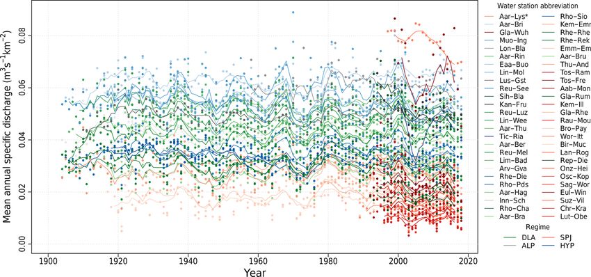
116                                                        A. Michel et al.: Evolution of stream temperature in Switzerland

dry months of the year. At the global scale, several studies      et al., 2005), but a linear relationship on longer timescales
have shown a clear trend over the last few decades with re-       (Lepori et al., 2015). The heat flux at the water surface is
spect to lake surface temperature (Dokulil, 2014; O’Reilly        composed of the solar radiation, the net longwave radiation,
et al., 2015) and stream temperature at various locations         and the latent and sensible (turbulent) heat fluxes. Studies
(Webb, 1996; Morrison et al., 2002; Hari et al., 2006; Han-       have shown that the main components of the total energy
nah and Garner, 2015; Watts et al., 2015). Evidence of spring     budget are the radiative components (Caissie, 2006; Webb
warming induced by earlier snow melt has been found in            et al., 2008). Friction at the stream bed and stream bed–water
North America (Huntington et al., 2003), and in Austria, a        heat exchanges have been shown to be non-negligible com-
country with similar climatic and geographical conditions to      ponents in some cases, e.g. steep slopes and altitudinal gra-
Switzerland, a clear warming has been observed throughout         dients (Webb and Zhang, 1997; Moore et al., 2005; Caissie,
the 20st century for all seasons, with the most marked in-        2006; Küry et al., 2017). These heat exchanges are more im-
crease in summer (Webb and Nobilis, 2007). A mean trend of        portant in the total heat budget in autumn when residual heat
+0.3 ◦ C per decade has been observed in England and Wales        from summer is still stored in the ground and when riparian
over the period from 1990 to 2006 by analysing more than          vegetation is present. In the latter case, induced shading and
2700 stations (Orr et al., 2015). A similar mean trend is found   reduced wind velocity decrease surface turbulent heat fluxes.
in Germany for the period from 1985 to 2010 over 132 sites           Groundwater temperature is also an important factor, es-
(Arora et al., 2016). While the warming is more pronounced        pecially close to the river source (Caissie, 2006) or in areas
in summer in Germany and in France (Moatar and Gailhard,          of significant groundwater infiltration. In Switzerland, this is
2006), the results in Wales and England show the opposite         especially important for high alpine rivers, which are mainly
with a stronger warming in winter.                                fed by glacier or snow melt, and are therefore sensitive to
   Over the last 50 years, a general warming trend has been       changes in the amount of melting and in seasonality (Har-
observed in Swiss rivers (FOEN, 2012) with a singular-            rington et al., 2017; Küry et al., 2017). Discharge is an im-
ity in 1987/1988: an abrupt step change of about +1 ◦ C           portant driver of water temperature; at different stream flow
(Hari et al., 2006; FOEN, 2012). This corresponds to the          stages, different water sources (soil water, groundwater, and
global climate regime shift observed during the same pe-          overland flow) contribute to the total discharge. Streamflow
riod (Reid et al., 2016; Serra-Maluquer et al., 2019). This       volume directly influences the heat balance as the wetted
warming is more pronounced in winter, spring, and sum-            perimeter of the river modifies atmospheric and ground heat
mer than in autumn (North et al., 2013). For the period           exchanges (Caissie, 2006; Webb and Nobilis, 2007; Toffolon
from 1972 to 2001, no general trend is observed before            and Piccolroaz, 2015) and the volume influences the tem-
or after the abrupt 1987/1988 warming (Hari et al., 2006).        perature change for a given amount of heat exchanged. Ac-
However, for some rivers, a clear trend exists in addition to     cordingly, discharge influences water temperature in a po-
the 1987/1988 shift. For example, the Rhine River in Basel        tentially highly non-linear way. This partly explains why
shows an increase of about +3 ◦ C between 1960 and 2010           many statistics-based water temperature models do require
(FOEN, 2012), and for rivers feeding into Lake Lugano, an         discharge as an explanatory variable (Gallice et al., 2016;
increase between +1.5 and +4.3 ◦ C has been observed for          Toffolon and Piccolroaz, 2015).
the period from 1979 to 2012 (Lepori et al., 2015). The              Anthropogenic influences on stream temperature have
1987/1988 shift is also observed in groundwater temperature,      been observed due to urbanization and channelization
but is more attenuated in time than that detected in surface      (Webb, 1996; Lepori et al., 2015), vegetation removal (John-
water temperature (Figura et al., 2011). The main driver of       son and Jones, 2000; Moore et al., 2005), the use of water for
the observed river warming in Switzerland is air tempera-         industrial cooling (Webb, 1996; Råman Vinnå et al., 2018),
ture, with the 1987/1988 increase due to the shift in North       or intake for agricultural irrigation (Caissie, 2006). Hydro-
Atlantic Oscillation and Atlantic Multi-decadal Oscillation       peaking (the sudden release of water at sub-daily timescale
indices (Hari et al., 2006; Figura et al., 2011; Lepori et al.,   from hydropower plants) and related thermopeaking have
2015). However, urbanization is also considered to be an ad-      been shown to reduce the impact of summer heat waves on
ditional driver in some catchments due to the increasing frac-    stream temperature (Feng et al., 2018); however, the effects
tion of sealed surfaces absorbing more radiative energy than      of these processes on aquatic life are so far relatively poorly
natural surfaces and transferring this heat to surface runoff     known (Zolezzi et al., 2011). Overall, most human influences
(Lepori et al., 2015).                                            have been proven to modify the relationship between air and
   Water temperature is the main focus of the research under-     water temperature, leading to a weaker correlation (Webb
lying this paper, although discharge evolution is also inves-     et al., 2008).
tigated as it is an important factor regarding the stream tem-       In this paper, we investigate the evolution of stream tem-
perature (Vliet et al., 2011). From a general perspective, the    perature and discharge in Switzerland for 52 catchments
main proxy for water temperature is air temperature, with a       since the beginning of measurement networks in the 1900s
clear non-linear relationship at a sub-yearly scale (such re-     (in the 1960s for water temperature) covering a variety of
lationships often show typical seasonal hysteresis; Morrill       landscapes from high alpine to lowland hydrological sys-

Hydrol. Earth Syst. Sci., 24, 115–142, 2020                                      www.hydrol-earth-syst-sci.net/24/115/2020/
A. Michel et al.: Evolution of stream temperature in Switzerland                                                             117

tems. Analysis is carried out on raw data for the whole time       to the best of our knowledge, no other Swiss canton pro-
period, and a linear regression analysis is performed over two     vides water temperature measurements before 2000. In par-
periods, 1979–2018 and 1999–2018. Trends in water tem-             ticular, no data from the canton of Ticino could be used (be-
perature, along with trends in discharge, air temperature, and     cause temperature measurements by the canton only started
precipitation are analysed using de-seasonalized time series.      after 2000); therefore, only one catchment is located on the
The 1987/1988 water temperature shift described in the lit-        southern side of the Alps in this study. Note that a recent
erature (Hari et al., 2006; Figura et al., 2011; North et al.,     study has already discussed the river warming in Ticino (Lep-
2013) is discussed in the context of extended historical time      ori et al., 2015).
series. Given the variety of fluvial regimes (alpine, lowland,        The 52 selected watersheds, presented in Table 1 and
and disturbed) found in Switzerland, the sensitivity of wa-        Fig. 1, cover a wide range of catchment areas (from a few
ter temperature change to this parameter is also examined.         square kilometres to tens of thousands of square kilometres)
Sensitivity to other topographical characteristics such as the     and mean elevations (from 450 m to more than 2500 m). Due
mean catchment elevation and surface area as well as the           to the complex topography of the country, the partitioning
fraction of glacier coverage are also investigated. The anal-      between solid and liquid precipitation can vary strongly over
ysis is carried out at a yearly and seasonal scales. Despite       small distances. Combined with the presence of glaciers in
the availability of the data sets, they have thus far not been     some catchments, this factor naturally influences the hydro-
analysed at such scale (52 catchments) and at a sub-yearly         logical response characterized via the hydrological regime
resolution in the context of climate change, especially with a     (Aschwanden et al., 1985). The selected catchments are
focus on the response of the different hydrological regimes.       representative of all natural hydrological regimes found in
In addition, the effect of lakes on river water temperature and    Switzerland except the southern Alps regimes; they can also
the memory effect in the hydrological system (influence from       be influenced by human activities (hydropower production,
season to season) are studied. Various effects including snow      lake regulation, and water intake or release). The basins are
melt or glacier retreat are also discussed, and some relevant      classified into four different categories (Piccolroaz et al.,
indicators for Switzerland are presented.                          2016):
   This study develops the first comprehensive analysis of
stream temperature and related variables in Switzerland,             – Swiss Plateau/Jura regime (SPJ): in the lower part of the
identifying changes to date and providing a reference for              country, most of the precipitation falls as rain. The hy-
gauging future evolution and scenarios in view of ongoing              drological response is driven by precipitation and evap-
climate change.                                                        otranspiration. The annual cycle with respect to dis-
                                                                       charge is moderate with a minimum in summer and ex-
                                                                       hibits high interannual variability depending on regional
                                                                       precipitation patterns.
2     Description of data
                                                                     – Alpine regime (ALP): at higher elevations, both the dis-
2.1    Stream temperature and discharge data                           charge and thermal regimes are strongly influenced by
                                                                       snow and glacier melt. A pronounced annual cycle is
Water temperature and discharge data as well as physio-                identifiable, with a maximum between March and July
graphic characteristics are provided by the Swiss Federal Of-          depending on the mean basin elevation and on the frac-
fice for the Environment (FOEN, 2019), by the Canton of                tion of glacier coverage, and a minimum during the win-
Bern Office of Water and Waste Management (AWA, 2019)                  ter season.
and by the Canton of Zurich Office of Waste, Water, En-
ergy and Air (AWEL, 2019). The discharge and water tem-              – Downstream lake regime (DLA): Switzerland has many
perature data from FOEN are provided at a daily time step,             large lakes, and most of them are regulated for flood
whereas the AWA and AWEL water data are provided at an                 control purposes (with the notable exception of Lake
hourly time step. For most of the FOEN stations, hourly data           Constance). As a result, downstream rivers are not only
also exist (see Table 1). While discharge measurements ex-             influenced by the lake itself (a natural buffer) but also
ist for some stations since the beginning of the 20th cen-             by its anthropogenic management (extra smoothing).
tury (mainly installed in the context of hydropower infras-
tructure projects), water temperature records only begin from        – Regime strongly influenced by hydro-peaking (HYP):
the 1960s. In the present study, stations with sufficiently long       roughly 55 % of Switzerland’s electricity production
times series of water temperature and discharge are selected           stems from hydropower plants (Schaefli et al., 2019).
(observations available since before 1980 for FOEN data and            Storage facilities at high elevation impact the hydrologi-
before 2000 for AWA and AWEL data). Some stations that                 cal regime in the lowlands due to controlled intermittent
fulfil these a priori conditions have been removed for other           release of large volumes of cold water.
reasons, which are detailed in Table S1 in the Supplement.
Data from other Swiss cantons have been investigated, but

www.hydrol-earth-syst-sci.net/24/115/2020/                                        Hydrol. Earth Syst. Sci., 24, 115–142, 2020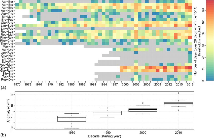
Table 1. Physiographic characteristics and data availability for water temperature and discharge of the 52 selected catchments. The IDs are those used by the data providers, and the
A. Michel et al.: Evolution of stream temperature in Switzerland
www.hydrol-earth-syst-sci.net/24/115/2020/
IDs followed by an asterisk represent stations where no hourly temperature measurements were available. The providers are the Swiss Federal Office for the Environment (FOEN), the
Canton of Bern Office of Water and Waste Management (AWA), and the Canton of Zurich Office of Waste, Water, Energy and Air (AWEL). For each basin, the selected representative
MeteoSwiss meteorological stations are indicated. The details of the abbreviations for the MeteoSwiss stations can be found in Table S2.
ID River Abbreviation Temperature Discharge Area Mean basin Glacier Hydrological Data Meteorological
measurement measurement (km2 ) elevation (m) surface (%) regime provider station
527 Aabach in Mönchaltorf Aab-Mon 1992–2018 1992–2018 46 523 0 SPJ AWEL SMA
2135 Aare in Bern Aar-Ber 1971–2018 1918–2018 2941 1596 5.8 DLA FOEN BER, INT
2019 Aare in Brienzwiler Aar-Bri 1971–2018 1905–2018 555 2135 15.5 HYP FOEN GRH, MER
2016 Aare in Brugg Aar-Bru 1963–2018 1916–2018 11 681 1000 1.5 DLA FOEN WYN, SMA
2029 Aare in Brügg–Aegerten Aar-Bra 1963–2018 1989–2016 8249 1142 2.1 DLA FOEN BER, MUB, PAY, NEU
2085 Aare in Hagneck Aar-Hag 1971–2018 1984–2018 5112 1368 3.4 DLA FOEN BER, MUB
2457 Aare in Ringgenberg Aar-Rin 1964–2018 1931–2016 1138 1951 12.1 DLA FOEN MER, INT
2030 Aare in Thun Aar-Thu 1971–2018 1906–2018 2459 1746 6.9 DLA FOEN MER, INT
A019 Alte Aare in Lyss Aar-Lys 1997–2018 1997–2018 13 462 0 SPJ AWA MUB, BER
2170 Arve in Geneva Arv-Gva 1969–2018 1904–2018 1973 1370 5 ALP FOEN GVE
2106 Birs in Münchenstein Bir-Muc 1972–2018 1917–2018 887 728 0 SPJ FOEN BAS, DEM
2034 Broye in Payerne Bro-Pay 1976–2018 1920–2018 416 715 0 SPJ FOEN PAY
A062 Chrouchtalbach in Krauchthal Chr-Kra 1999–2018 1999–2018 16 702 0 SPJ AWA BER
2070 Emme in Emmenmatt Emm-Emm 1976–2018 1974–2018 443 1065 0 SPJ FOEN LAG, NAP
2481 Engelberger Aa in Buochs Eaa-Buo 1983–2018 1916–2018 228 1609 2.5 HYP FOEN ENG
522 Eulach in Winterthur Eul-Win 1993–2018 1993–2018 64 541 0 SPJ AWEL SMA, TAE
2415 Glatt in Rheinfelden Gla-Rhe 1977–2018 1976–2018 417 503 0 SPJ FOEN SMA, KLO
534 Glatt in Rümlang Gla-Rum 1992–2018 1992–2018 302 520 0 DLA AWEL SMA
531 Glatt in Wuhrbrücke Gla-Wuh 1993–2018 1993–2018 64 621 0 SPJ AWEL SMA
2462 Inn in S-Chanf Inn-Sch 1981–2018 1999–2018 616 2463 6.1 ALP FOEN SAM, SIA, BEH
A017 Kander in Frutigen Kan-Fru 1995–2018 1992–2018 180 2156 14 ALP AWA ABO
517 Kempt in Illnau Kem-Ill 1992–2018 1992–2018 37 615 0 SPJ AWEL SMA, TAE
2634∗ Kleine Emme in Emmen Kem-Emm 1973–2018 1936–2018 478 1054 0 SPJ FOEN LUZ, NAP
Hydrol. Earth Syst. Sci., 24, 115–142, 2020
A025 Langete in Roggwil Lan-Rog 1996–2018 1996–2018 130 689 0 SPJ AWA KOP, WYN
2243 Limmat in Baden Lim-Bad 1969–2018 1951–2018 2384 1131 0.7 DLA FOEN SMA, WAE
2372 Linth in Mollis Lin-Mol 1964–2018 1914–2018 600 1743 2.9 HYP FOEN ELM, GLA
2104 Linth in Weesen Lin-Wee 1964–2018 1907–2018 1062 1584 1.6 DLA FOEN ELM, GLA RAG
2269 Lonza in Blatten Lon-Bla 1967–2018 1956–2018 77 2624 24.7 ALP FOEN ABO, GRH
A070 Luterbach in Oberburg Lut-Obe 1994–2018 1994–2018 34 700 0 SPJ AWA BER
2109 Lütschine in Gsteig Lus-Gst 1964–2018 1908–2018 381 2050 13.5 ALP FOEN INT, GRH
2084 Muota in Ingenbohl Muo-Ing 1974–2018 1917–2018 317 1363 0 HYP FOEN ALT
A029 Önz in Heimenhausen Onz-Hei 1994–2018 1995–2018 86 582 0 SPJ AWA KOP, WYN
A031 Ösch in Koppigen Osc-Kop 1997–2018 1997–2018 39 559 0 SPJ AWA KOP
A049 Raus in Moutier Rau-Mou 1997–2018 1997–2018 41 896 0 SPJ AWA DEM
572 Reppisch in Dietikon Rep-Die 1993–2018 1993–2018 69 594 0 DLA AWEL SMA
2152 Reuss in Luzern Reu-Luz 1973–2018 1922–2018 2254 1504 2.8 DLA FOEN LUZ
2018 Reuss in Mellingen Reu-Mel 1969–2018 1904–2018 3386 1259 1.8 DLA FOEN LUZ, SMA
2056 Reuss in Seedorf Reu-See 1971–2018 1904–2018 833 2013 6.4 HYP FOEN ALT
2473 Rhein in Diepoldsau Rhe-Die 1970–2018 1919–2018 6299 1771 0.7 HYP FOEN CHU, RAG, VAD
118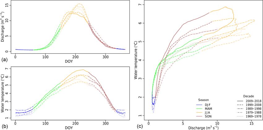
A. Michel et al.: Evolution of stream temperature in Switzerland 119
2.2 Meteorological data
One or more meteorological stations, operated by the Fed-
eral Office of Meteorology and Climatology (MeteoSwiss),
have been associated to each hydrometric gauging station
KLO, SAE, STG
SIO, GRC, GRH
Meteorological
(IDAWEB, 2019). These meteorological stations were se-
MUB, BER
SMA, TAE
SMA, TAE
HLL, KLO
CDF, CHA
BAS, KLO
lected according to the proximity of the catchments in order
WAE, EIN
SBE, OTL
SIO, GSB to be representative of the local meteorological conditions.
station
GVE
BER
Only stations with sufficiently long data records at a daily
timescale were kept.
Daily measurements of air temperature and precipitation
provider
AWEL
AWEL
AWEL
FOEN
FOEN
FOEN
FOEN
FOEN
FOEN
FOEN
FOEN
were compiled, and homogeneous time series (Füllemann
AWA
AWA
Data
et al., 2011) were used whenever available. Homogenization
carried out by MeteoSwiss consists of adjusting historic mea-
Hydrological
sured values to current measuring standards and locations.
Figure 1 shows a map detailing all of the hydrological mea-
regime
DLA
DLA
DLA
DLA
HYP
HYP
HYP
surement sites and the associated MeteoSwiss stations. In to-
SPJ
SPJ
SPJ
SPJ
SPJ
SPJ
tal, 41 MeteoSwiss stations are associated with one or several
catchments. Details on the stations are given in Table S2.
Glacier
surface (%)
0.4
1.1
8.3
11.1
14.2
0
0
0
0
0.1
0
0
0
2.3 Snow water equivalent and glaciers mass balance
Monthly snow water equivalent maps of Switzerland are
used as a proxy for snow melt. These maps are provided
Mean basin
elevation (m)
1131
1068
1569
2127
2291
459
1168
1080
770
1643
626
803
666
by the WSL Institute for Snow and Avalanche Research
SLF. They are generated using a temperature-index model
in which observational SWE data are assimilated using an
ensemble Kalman filter (Magnusson et al., 2014; Griessinger
et al., 2016). Glacier annual and seasonal (summer and win-
Area
(km2 )
14 767
34 524
10 308
5238
3372
13
102
61
1702
1613
399
127
67
ter) mean local mass balance and surface extent are available
for selected glaciers from the GLAMOS data set (GLAMOS,
measurement
2018). The mass balance is estimated based on in situ
1904–2018
1933–2018
1904–2017
1905–2018
1916–2018
1996–2018
1992–2018
1995–2018
1904–2018
1997–2018
1992–2018
1992–2018
1989–2018
Discharge
biannual measurements and then extrapolated to the whole
glacier area using distributed modelling and point measure-
ment homogenization techniques (Huss et al., 2015) to re-
trieve the mean local mass balance. The total mass balance
measurement
Temperature
is obtained in this study by multiplying the mean annual and
1969–2018
1971–2018
1968–2018
1974–2018
1996–2018
1992–2018
1995–2018
1963–2018
1978–2017
1992–2018
1992–2018
1989–2018
1971-2017
seasonal mass balance (in millimetres water equivalent per
year) by the glacier area.
Abbreviation
3 Methods
Thu-And
Tos-Ram
Rho-Cha
Rhe-Rek
Rhe-Rhe
Sag-Wor
Rho-Pds
Rho-Sio
Tos-Fre
Sih-Bla
Suz-Vil
Tic-Ria
Wor-Itt
3.1 Data preprocessing procedure
In the analysis below, only complete calendar years are re-
tained; sparse or missing data are allowed as long as gaps
Rhône in Porte du Scex
Rhein in Rheinfelden
Töss in Ramismuhle
Thur in Andelfingen
do not exceed 2 weeks. For daily averaging, missing data are
Sagibach in Worben
Töss in Freienstein
Rhein in Rekingen
Ticino in Riazzino
Rhône in Chancy
Worble in Ittigen
propagated (i.e. one missing data point during a day results
Sihl in Blattwag
Suze in Villeret
Rhône in Sion
in a missing day), but they are ignored for seasonal and an-
nual averaging. Seasonal and annual time series are used for
Table 1. Continued.
all interannual comparisons and for inter-variable correlation
River
studies. Daily time series are used for the trend analysis. In-
deed, more points are available for daily values than for an-
2091*
2011∗
nual values, leading to more robust trends (see Sect. 3.3).
A047
A022
2143
2174
2009
2044
2068
2500
547
570
520
ID
www.hydrol-earth-syst-sci.net/24/115/2020/ Hydrol. Earth Syst. Sci., 24, 115–142, 2020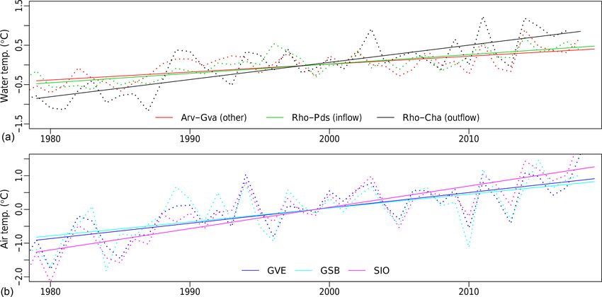
120 A. Michel et al.: Evolution of stream temperature in Switzerland
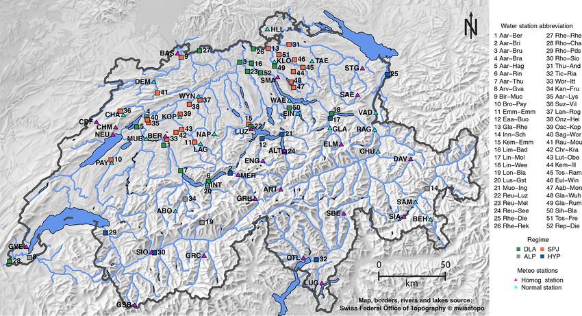
Figure 1. Map of Switzerland showing the selected hydrometric gauging stations and the associated meteorological stations. Abbreviations
for hydrometric gauging stations are defined in Table 1, and abbreviations for the meteorological stations are given in Table S2.
3.2 Seasonal signal removal and Devlin, 1988; Cleveland et al., 1988) is defined by the
tricubic function:
Before applying linear regression to daily data, the seasonal
3 3 for 06x < 1
signal is removed using a method called seasonal-trend de- W (x) = 1 − x . (2)
composition based on “loess” (STL) (Cleveland et al., 1990), 0, otherwise
where loess stands for “locally weighted regression” (Cleve-
Therefore W (x) is large for xi close to x and becomes zero
land and Devlin, 1988; Cleveland et al., 1988). This method
for xi further than the qth farthest point. We can see that
is robust with respect to outliers in the time series, able to
q will act as a smoothing parameter on the fit obtained with
cope with missing data and with any seasonal signal shape,
this method.
and is computationally efficient. In addition, the seasonality
In the STL algorithm, vectors of data Y are decomposed
is allowed to change over time and this rate of change is pa-
as follows:
rameterized by the user. The STL method has been widely
used in other fields; examples of application in hydrology in- Yi = Ti + Si + Ri , (3)
clude the work of Hari et al. (2006), Figura et al. (2011), or
Humphrey et al. (2016). where Ti is the trend term, Si the seasonal term, and Ri the
Here, only the main ideas of the method are presented; residual term. The algorithm is composed of two iterative
full details are given in Cleveland et al. (1990). The loess loops, called inner and outer loops. In the inner loop, the time
fitting method is a local fitting with weights applied to the series is first de-trended: Ti is extracted and smoothed with
points that are fitted. The fitting can be locally linear or lo- a loess fitting as explained above. Then, the seasonal com-
cally quadratic, here we use the locally linear fitting follow- ponent is extracted using a low-pass filter, and the remaining
ing Cleveland et al. (1990). For any xi in the neighbourhood time series is again smoothed by loess. This process is re-
of x, the loess, or the weight applied to the points before car- peated iteratively and encapsulated in an outer loop. In this
rying out a local fitting, is defined as follows: second loop, a weight is attributed to each point based on its
residual (i.e. Yi − Ti − Si ) such that the weight is low when
|xi − x| the residual term is large. These weights are used for the loess
v(x) = W . (1)
λq (x) fitting in the next round of the inner loop. As the outliers are
given a low or zero weight, the method is robust to the pres-
Note that xi is the position of the point, not its value. λq (x) is ence of outliers. At the end of the loop, Ri is obtained by
defined as the distance to the qth furthest point, with q being subtracting the final Ti and Si from the raw data. Note that
a parameter of the model discussed below. W (x) (Cleveland the trend term obtained here is a locally fitted function, so
Hydrol. Earth Syst. Sci., 24, 115–142, 2020 www.hydrol-earth-syst-sci.net/24/115/2020/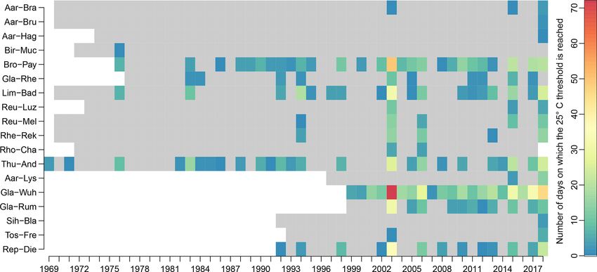
A. Michel et al.: Evolution of stream temperature in Switzerland                                                              121

it is completely different from the regression parameters ob-      ns = 37, for all variables and all catchments. A single value
tained by a linear regression, which will later be called the      for all catchments and variables is preferable. Indeed, as this
trend.                                                             value defines how the signal can evolve over time, and thus
    The STL method has five algorithmic parameters: the            influences the trend and the residual terms, different values
number of iterations in the inner loop (ni ), the number of        would make the comparison of linear regression output be-
iterations in the outer loop (no ), the smoothing parameter        tween catchments and variables less relevant.
of the low-pass filter (nl ), the smoothing parameter of the          Some example outputs of the STL method and additional
trend component (q), and the seasonal smoothing parameter          details are given in Sect. S1.3 of the Supplement. It is note-
(ns ). The value of parameter nl is imposed by the time series     worthy that the de-seasonalization with the STL method has
sampling frequency and is set here to 365, which is the least      almost no effect on precipitation. However, in Fig. S4 in the
odd integer greater than or equal to the time series frequency.    Supplement, we show that the seasonality in precipitation
The parameters ni and no are set to the recommended values,        time series is weak.
i.e. ni = 1 and no = 15 (Cleveland et al., 1990). Following
the same recommendation, the parameter q is defined as the         3.3   Linear regression
first integer respecting the following condition:
       1.5np                                                       The temporal trends are explored using linear regressions
q≥             −1
                  ,                                         (4)    over different time periods, which has been shown to be
     1 − 1.5ns                                                     a suitable approach (Lepori et al., 2015) and is commonly
where np is the time series frequency.                             used (Hari et al., 2006; Schmid and Köster, 2016). A lin-
    For the seasonal smoothing parameter ns , no formal rec-       ear regression is applied to all four de-seasonalized variables
ommendation based on previous mathematical analyses ex-            (i.e. Ti + Ri from the STL method, for the water tempera-
ists (Cleveland et al., 1990). This parameter determines the       ture, discharge, air temperature, and precipitation variables)
variation of the seasonal signal over time and thus the frac-      against time with the classical least-squares estimation tech-
tion of the data variation that is included in the seasonal com-   nique. The linear model is applied, when possible, for the
ponent. If set to a small value, the seasonal component will       1979–2018 and 1999–2018 periods.
vary greatly from year to year, including interannual variabil-       As expected, the correlation determination R 2 values are
ity. If set to an overly large value, the seasonal component       relatively low, because the daily and interannual variability
will be exactly the same from year to year, and the method         is still present in the time series and the linear model cannot
is no longer superior to a simple periodic removal of the sea-     represent these components. However, the p values are all
sonal signal (as classically done in hydrological time series      very small, and the residuals of the linear model show that,
analysis, e.g. in Schaefli et al., 2007). The method proposed      for all periods, the linear regression against time only is a
by Cleveland et al. (1990) to adjust this parameter is not ap-     suitable estimator of the trend.
plicable here: it would require an assessment based on 365            The robustness of the trends is assessed using two in-
different plots per catchment. We propose here to use the          dependent methods. The first method compares the results
autocorrelation function (ACF) and the partial autocorrela-        from the simple linear model to a robust linear model (Ham-
tion (PACF) of the residuals’ time series to select an appro-      pel, 1986). This model, which is less sensitive to outliers,
priate ns . In fact, the ACF and the PACF can be used to ensure    is well suited for de-seasonalized temperature time series,
that no seasonality remains in the residuals. In particular, the   but has shown problems with the remaining variability in
ACF and the PACF of the residuals should not show any sig-         the de-seasonalized discharge and precipitation time series,
nificant correlation at the biannual (183 d) or the annual scale   including convergence problems for precipitation. For our
(365 d), as this would be indicative of seasonal components        case study, this method fails to converge for all precipitation
being left in the residuals.                                       time series. The differences in trends obtained by the simple
    Therefore, the following method is applied to all wa-          and robust linear models for the four variables are shown in
ter temperature, discharge, air temperature, and precipitation     Figs. S9 and S10. The only notable difference is for discharge
time series: the STL is run for ns ranging from 7 to 99 (note      during the 1999–2018 period.
that ns has to be odd and ≥ 7), and the ACF and PACF are              The second method, which assesses the sensitivity to
computed for all residuals’ time series. The mean ACF and          boundary effects, consists of removing 1 year at the begin-
PACF values for lags between 360 and 370 are plotted against       ning or at the end of the period and recompute the trends (re-
the ns value and the plots are checked individually by visual      moving 2 years leads to similar results). Figure S11 shows
inspection to determine the best ns . Visual inspection is jus-    the analysis for the 1999–2018 period. The trends for wa-
tified by the fact that for some catchments and variables, the     ter and air temperature are indeed lower when the last
PACF decreases monotonically and tends to a constant value,        year (2018, which was extremely warm in Switzerland) is
whereas in other cases, it reaches a minimum before increas-       removed, whereas for discharge and precipitation the nega-
ing again, making an automated decision process difficult.         tive trends are less pronounced when the first year (1999) is
Based on this analysis, the value retained for this study is       removed. These differences are notable, but do not change

www.hydrol-earth-syst-sci.net/24/115/2020/                                        Hydrol. Earth Syst. Sci., 24, 115–142, 2020
122 A. Michel et al.: Evolution of stream temperature in Switzerland
the main message of the study. For the 1979–2018 period, The indicator is computed following a simple approach
removing 1 year, both at the beginning or at the end of the inspired by the more complex model proposed in the work
time interval, leads to negligible differences, showing the of Carraro et al. (2016). First, the days on which the water
overall robustness of the trends computed over 40 years (see temperature remains above 15 ◦ C for the whole day are com-
Fig. S12). puted (a 3 h moving window average is applied beforehand).
The root-mean-square error (RMSE) of the trends ob- Then, data are filtered to keep only series longer than 28 con-
tained over a shorter period is used as a measure of the uncer- secutive days. Finally, the number of days above 28 days in
tainty of the mean trend values (the largest RMSEs between the remaining series are summed for each year. The results
trends obtained by removing 1 year at the beginning or at indicate the number of days in the year for which the temper-
the end are used as the uncertainty value). For single trend ature was above 15 ◦ C for at least 28 consecutive days. As
uncertainty, the largest difference between the normal linear the process behind PKD is far more complex, this method
model trend and trends obtained by removing 1 year at the does not pretend to be exact in determining the presence or
beginning or at the end is used as the uncertainty value (indi- absence of PKD in the rivers monitored; however it is an
cated in Tables A1, A2, S4, and S5). indicative approach to assess the exposure evolution of the
The linear regressions are also applied to seasonal and an- river system. A sensitivity analysis has been performed and
nual mean time series. In this case, the R 2 values are clearly the qualitative evolution is not dependent on the chosen val-
higher, as there is less variance in the input data, but the ues for the period length and for the moving average window
p values increase. Indeed, only 20 or 40 points are used size.
depending on the time period, reducing the robustness of
the method. Some p values are even above the significance
threshold. As a consequence, the long-term trends presented 4 Results and discussion
in this paper only use de-seasonalized time series, with p val-
ues < 0.05. Seasonal trends, obtained from seasonal mean 4.1 Long-term evolution of stream temperature and
values, must be interpreted cautiously. As a consequence, discharge
most of the seasonal analysis is based on raw seasonal means
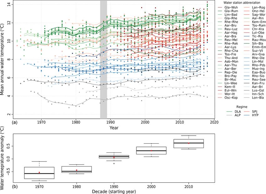
instead of trends due to their low significance level. The water temperature evolution for all gauging stations used
For catchments with more than one meteorological sta- in the current study is shown in Fig. 2a. In spite of the
tion attributed to them, the trends used in the analysis for air high natural variability, a warming trend is visible in most
temperature and precipitation are the mean of the trends of rivers. To investigate this evolution in detail, catchments with
all the catchment’s stations. For precipitation and discharge, temperature measurements available since 1970 are selected
they are expressed in relative changes to allow for a compar- (14 catchments). Figure 2b shows the temperature anoma-
ison between catchments. Unless stated explicitly, trends are lies per decade with respect to the 1970–2018 mean for these
expressed per decade. catchments. A two-sided t test is performed to assess if the
differences in decadal means are significant. Except between
3.4 Ecological indicators the 1970s and 1980s, where no significant difference is found
(p value = 0.17), all of the other respective anomaly means
Two important ecological indicators are used to quantify the are shown to be significantly different (p values < 5 × 10⁻⁵
impact of river warming and its evolution: the number of for the three tests) which confirms the important rise ob-
days on which stream temperature reaches or exceeds the served since 1980 (Fig. 2b). The shift occurring at the end
value of 25 ◦ C, and the number of consecutive days during of the 1980s reported by Hari et al. (2006) and discussed in
which the hourly temperature remains above 15 ◦ C. Figura et al. (2011) and Lepori et al. (2015) is not observed
The 25 ◦ C threshold is a legal limit in Switzerland above in all rivers (see Fig. 2a). Indeed, the shift is clearly visible
which heat release in rivers is forbidden; this is important, in catchments located in the Swiss Plateau/Jura regions and
for example, for nuclear power plant cooling. The indicator downstream lakes, but not necessarily in alpine catchments
is computed as follows: based on hourly data, when the water or catchments strongly influenced by hydro-peaking. Note
temperature reaches 25 ◦ C for at least 1 h, the day is flagged that this shift is also present in air temperature records (see
as being above 25 ◦ C. Then, the number of such days per year Fig. S13). The shift between the 1980s and 1990s is more im-
are summed in order to investigate the evolution over time. portant than previous or subsequent shifts, but contrary to the
The 15 ◦ C threshold is important for fish health. Indeed, statement in Hari et al. (2006), the warming trend continues
proliferative kidney disease (PKD) affecting salmonid fish is after the shift. Looking at the 30-year anomaly difference,
caused by a parasite that proliferates when the water temper- the mean anomaly difference over the 14 catchments for the
ature remains above 15 ◦ C for a few weeks (Hari et al., 2006; 1970–2000 period is 0.59 ◦ C and for the 1990–2018 period
Carraro et al., 2016, 2017). Thus, water temperature affects it is 0.55 ◦ C. A partially overlapping samples two-sided t test
the impact of PKD and its prevalence (Carraro et al., 2017). (Derrick et al., 2017) finds no significant difference between
these two values (p value = 0.59, this test is used instead of
Hydrol. Earth Syst. Sci., 24, 115–142, 2020 www.hydrol-earth-syst-sci.net/24/115/2020/A. Michel et al.: Evolution of stream temperature in Switzerland 123
a classic t test as the two samples overlap). Consequently, to boundary effects and the generally higher robustness of
the “end-of-80s” shift might be interpreted as a hiatus in the linear regressions over longer time periods.
long-term trend. The apparent acceleration of the warming Trends in stream temperature and discharge are compared
seen over recent years is due to the extreme year 2018, which to trends in air temperature and precipitation in Fig. 5. There
pulls up the running mean. is a clear increase in water temperature and a reduction in dis-
A long-term analysis is also performed on discharge data charge observed in Swiss rivers over the 1999–2018 period.
(Fig. 3). In this case, catchments with measurements ranging The mean trends for the last 20 years are +0.37 ± 0.11 ◦ C
back to at least 1920 (20 catchments) are kept for anomaly per decade for water temperature (with a large spread in the
analysis. Figure 4 shows that there is almost no trend in the distribution), +0.39±0.14 ◦ C per decade for air temperature,
long term for annual mean discharge and precipitation (for −10.1±4.6 % per decade for discharge, and −9.3±3.4 % per
the discharge, the mean trend obtained by linear regression decade for precipitation. However, the trends in precipitation
over the 26 catchments available between 1970 and 2018 is and runoff have to be considered with caution regarding the
−0.5 % per decade). However, recent decades have shown a long-term variation discussed above. For the 1979–2018 pe-
clear negative trend. The 1980s exhibited a positive runoff riod, the mean trends are as follows: +0.33 ± 0.03 ◦ C per
anomaly with a decrease toward the end of the decade. A decade for water temperature (again with a large spread in the
7- to 8-year cycle in the runoff annual mean can be seen in distribution), +0.46 ◦ C ± 0.03 ◦ C per decade for air tempera-
Fig. 3. This is related to the cycle found in the North Atlantic ture, −3.0±0.5 % per decade for discharge, and −1.3±0.5 %
Oscillation (NAO) and the Atlantic Multi-decadal Oscilla- per decade for precipitation.
tion (AMO) which has already been discussed in the litera- The water temperature and discharge trends for the four
ture (Lehre Seip et al., 2019). These cycles also have an in- different regimes are shown in Fig. 6. Similar plots for air
fluence on water temperature as shown by Webb and Nobilis temperature and precipitation are shown in Fig. S14. A two-
(2007). The time series are presented in Fig. S15. sided Wilcoxon test is used to assess whether differences be-
A longer multi-decadal variation can be seen in discharge tween regimes are significant in terms of temperature trends
data (see Fig. 4). However, 1 century of data is not long (results shown in Table S3). As some categories only have
enough to assess if there is a real 30- to 40-year cycle, a few observations and normal distribution can not be as-
which could be related to the 34- to 36-year cycle found sumed, this test is used instead of a t test. Two groups can
in the Atlantic Meridional Overturning Circulation (AMOC) clearly be identified: the downstream lakes (DLA) regime
(Lehre Seip et al., 2019), or if there is only some statistical and the Swiss Plateau/Jura (SPJ) regime on the one hand,
variation. As a consequence, it is not possible to assess if the and the alpine (ALP) and hydro-peaking-influenced (HYP)
decrease over the last decade is part of a long-term cycle, if regimes on the other hand. Indeed, for both pairs of regimes,
it results from climate change, or both. the hypothesis of different mean values is clearly rejected
The decades from 1970 to 1980 and 1980 to 1990 show a with p values > 0.15 (i.e. testing the hypothesis of a different
more marked anomaly (negative first and then positive, see mean between SPJ and DLA and between HYP and ALP).
Fig. 4) for discharge than for precipitation. This is explained The water temperature trends are significantly lower for
by the glacier melt evolution, which reaches a minimum in alpine catchments and catchments strongly influenced by
the decade from 1970 to 1980 followed by a sharp increase hydro-peaking. The impact of lakes is discussed in Sect. 4.3.
in the next decade (Huss et al., 2009). The catchment area is not correlated with trend values (see
Fig. 6) despite the fact that area is clearly correlated with
the regime (Table 1). To infer the isolated effect of area,
4.2 Temperature and discharge trends from linear
only catchments from the Swiss Plateau/Jura regime are used
regression
(largest sample of rivers and no major disturbance), but no
correlation between water temperature or discharge trends
The trends in stream temperature and discharge have been and area can be found (see Fig. S19).
computed using linear regression over the 1999–2018 period Elevation and the fraction of glacier coverage in the catch-
for all 52 catchments and over the 1979–2018 period when ment (which are strongly correlated) clearly correlate with
possible. All trend values are presented in the Appendix in water temperature and discharge trends (see Fig. 6, bottom
Tables A1 and A2 for water temperature and discharge, and row). The smaller positive trends in water temperature and
in Tables S4 and S5 for air temperature and precipitation. reduced negative trends in discharge observed for highly
The plots shown in this section are for the 1999–2018 pe- glaciated catchments can be attributed to cold water coming
riod, where more catchments are available. Similar plots for from glacier melt (as discussed in Williamson et al., 2019),
the 1979–2018 period are shown in Sect. S2.1. Note that re- as air temperature trends for alpine catchments are similar
sults presented in this section, except for the trends in runoff to lowland catchments (see Fig. S14). For these reasons,
over the last few decades, also hold for the longer time pe- discharge and temperature of alpine streams have been the
riod, and the results are even more evident over this longer least impacted by climate change to date. However, if this
time period. This can be explained by the lower sensitivity buffer effect induced by glaciers and seasonal snow cover
www.hydrol-earth-syst-sci.net/24/115/2020/ Hydrol. Earth Syst. Sci., 24, 115–142, 2020124 A. Michel et al.: Evolution of stream temperature in Switzerland Figure 2. (a) Mean annual stream temperature of the 52 catchments described in Table 1. Lines show the 5-year moving averages. Colours indicate the hydrological regimes. The 1987/1988 transition period is highlighted using grey. Abbreviation for river names are given in Table 1, and abbreviations for regimes are as follows: DLA represents the downstream lake regime, ALP represents the alpine regime, SPJ represents the Swiss Plateau/Jura regime, and HYP represents the strong influence from hydro-peaking. (b) Water temperature anomalies per decade with respect to the 1970–2018 mean, for the 14 catchments with data available since 1970. Thick lines are the median and red dots the mean values (values used for the t test and the partially overlapping samples t test, see text). Boxes represent the first and third quartiles of the data, whiskers extend to points up to 1.5 times the box range (i.e. up to 1.5 times the distance of the first to third quartiles) and extra outliers are represented as circles. Figure 3. Mean annual specific discharge for the 52 catchments described in Table 1 (normalized by catchment area for comparison). Lines show the 5-year moving averages. Colours indicate the hydrological regimes. Values for the Alte-Aare (Alt-Lys, marked using an asterisk in the legend) are divided by 4 to fit in the plot. Hydrol. Earth Syst. Sci., 24, 115–142, 2020 www.hydrol-earth-syst-sci.net/24/115/2020/
A. Michel et al.: Evolution of stream temperature in Switzerland                                                                    125

Figure 4. Relative discharge (a) and precipitation (b) decadal means of anomalies with respect to the 1920–2018 average for 20 catchments
and 17 MeteoSwiss homogeneous stations with data available since 1920 (see Tables 1 and S2).

Figure 5. Water and air temperature trends (a) as well as normalized discharge and normalized precipitation trends (b) for the 1999–
2018 period and for the 52 catchments described in Table 1 and their associated meteorological stations.

disappears due to the continuation of temperature rise in the          the trends obtained with a linear model (boundary effects).
future (Bavay et al., 2013; Huss et al., 2014; MeteoSuisse             For ALP and HYP catchments, the general poor correlation
et al., 2018), the alpine catchments will be amply impacted            suggests that additional factors, such as snow and glacier
(see Sect. 4.4.4). Lowland catchments, mostly located in the           melt and anthropogenic disturbances, become predominant
Swiss Plateau/Jura regions, experience the most important              in the energy balance, decoupling the mean air temperature
decrease in discharge.                                                 and water temperature trends.
   Unsurprisingly, rivers strongly influenced by hydro-
peaking show lower temperature trends compared with                    4.3   Effect of lakes
undisturbed waterways. This results from large volumes of
cold water being released from reservoirs located at high el-          In the previous section, it was shown that rivers located
evation to lowland rivers as discussed, for instance, in Feng          downstream of lakes have water temperature trends similar to
et al. (2018).                                                         the Swiss Plateau/Jura catchments, in spite of a higher mean
   In conclusion, for Swiss Plateau/Jura catchments, air and           elevation and a larger glacier-covered fraction (see Table 1),
water temperature trend distributions are similar, and the             which typically attenuate the water temperature increase.
mean of the trends for this type of catchment is close to                 The effect of lakes located at the foot of mountain ranges
the mean air temperature trend (see Figs. 6 and S14). Fig-             on stream temperature is well known (Webb and Nobilis,
ures S20 and S21 show water temperature trends for each                2007; Råman Vinnå et al., 2018). The input water originates
catchment plotted against trends in air temperature for the            from alpine rivers (potentially disturbed by hydro-peaking),
1999–2018 and 1979–2018 periods. Single values (i.e. water             which are colder than the surrounding environment and not in
and air temperature trends for a given catchment) are poorly           equilibrium with local air temperature. As water has a certain
correlated. Over the 1979–2018 time period, a better correla-          residence time in the lake, its temperature increases due to at-
tion for DLA and SPJ catchments is visible, suggesting that            mospheric forcing and the main driver for the outflow water
part of the poor correlation in Fig. S20 is due to the noise in        temperature is the air temperature. However, it has currently
                                                                       not been demonstrated if the effect of lakes on river temper-

www.hydrol-earth-syst-sci.net/24/115/2020/                                             Hydrol. Earth Syst. Sci., 24, 115–142, 2020
126 A. Michel et al.: Evolution of stream temperature in Switzerland Figure 6. Water temperature and discharge trends for the 1999–2018 period classified by the four different hydrological regimes – down- stream lake regime (DLA), alpine regime (ALP), Swiss Plateau/Jura regime (SPJ), and strong influence from hydro-peaking (HYP) (top-left two panels); by the catchment area (top-right two panels); by the catchment mean elevation (bottom-left two panels); and by the glacier coverage (bottom-right two panels). The numbers along the bottom of the panels indicate the number of catchments in each category. In the top-left boxplot, the red dots are the mean values (values used for the Wilcoxon test, see text). Figure 7. (a) Lake Geneva water temperature anomalies and trends for inflow (Rho-Pds) and outlet (Rho-Cha) stations (a). Arv-GVA denotes the Arve in Geneva, Rho-Pds represents the Rhône in Porte du Scex, and Rho-Cha represents the Rhône in Chancy. (b) Air temperature anomalies and trends for surrounding MeteoSwiss stations. GVE denotes Geneva-Cointrin, GSB denotes Grand Saint-Bernard, and SIO denotes Sion. The period for trend computation is from 1979 to 2018. ature trends is similar. In Schmid and Köster (2016), it is Biel, Lake Luzern, Lake Walen, and Lake Geneva. Temper- shown that lake temperature trends can exceed air tempera- ature anomalies with respect to the 1979–2018 period and ture trends due to solar brightening. trends are plotted for water temperature at each station and To investigate the effect of lakes on water temperature air temperature at meteorological stations representative of trends, five lake systems with measurements at the inflow and the catchment. The results are shown in Fig. 7 for Lake the outlet are selected: the Thun–Brienz lake system, Lake Geneva and in Figs. S22 to S25 for the other four lakes. The Hydrol. Earth Syst. Sci., 24, 115–142, 2020 www.hydrol-earth-syst-sci.net/24/115/2020/
A. Michel et al.: Evolution of stream temperature in Switzerland                                                               127

trends for the different inflow and outflow rivers and for air     namics and, thus, are essential for inferring the impacts of cli-
temperature are presented in Table 2.                              mate change on water temperature and discharge. The anal-
   For Lake Walen and Lake Geneva, the effect is obvious:          ysis below is mostly based on the 1999–2018 period. Sea-
the outlet trend is almost equal to the co-located air tem-        sons are defined as follows: winter is December–January–
perature trend. Even if trends in inflows are much smaller,        February (DJF), spring is March–April–May (MAM), sum-
they do not significantly influence the outlet waters (see Ta-     mer is June–July–August (JJA), and autumn is September–
ble 2). The lake acts as catalyst and the system reaches a         October–November (SON).
quasi-equilibrium. For Lake Geneva, the water temperature             Long-term evolution of the seasonal anomalies are shown
of the Arve River is also shown. The Arve River originates         in Figs. 8 and 9 for water temperature (decades from 1970
from the Mont Blanc massif (France) and flows for about            to 2010) and discharge (decades from 1960 to 2010). Air
100 km through the Arve Valley before joining the Rhône in         temperature and precipitation are shown in Figs. S26 and S27
Geneva. Despite flowing through low-lying land, the Arve           and exhibit similar behaviour. For all seasons, the water tem-
keeps its alpine characteristics, whereas these characteristics    perature has been significantly rising since 1980. The warm-
are completely lost in the Rhône River after the lake.             ing is more important in summer and less pronounced in win-
   In Lake Luzern, a similar effect is observed. Indeed, the       ter. For discharge, spring and autumn do not show an obvious
three rivers feeding the lake (the Reuss, Muota, and Engel-        trend in the long term. There is a clear decrease in summer
berger Aa rivers) show trends that are considerably lower          since 1980, whereas winter shows a slight increase.
than that for the Reuss River in Luzern (see Table 2). How-           Annual and seasonal trends for stream and air temperature,
ever, the Kleine-Emme River, which joins the Reuss just after      discharge, and precipitation are presented in Fig. 10 for the
Luzern, shows a similar trend without the presence of a lake       1999–2018 period. They confirm the tendencies described
along its course; this demonstrates that, for a mid-elevation      above. Mean water temperature trends are slightly smaller
stream, flowing a certain distance on the Swiss Plateau leads      than air temperature trends for all seasons except for spring,
to a similar effect to that induced by lakes. For the Thun–        when they are notably larger. This shows that rivers do not re-
Brienz lake system, the water temperature trend is enhanced        act linearly to a general warming of the atmosphere and addi-
as a result of the two subsequent lakes and it gets closer to      tional factors control these complex systems. For discharge,
the air temperature trend.                                         negative trends are found in all seasons except for winter,
   For Lake Biel, no effect is observed. This is not surprising    when they are almost zero. Discharge trends follow precipita-
as the Aare input water already has a trend similar to the local   tion trends in all seasons. In general, precipitation determines
air temperature. In addition, the residence time in Lake Biel      the discharge trend; consequently, snow and glacier melt play
is very short (58 d, whereas for the five other lakes it ranges    a minor role in the observed trends. However, for specific
from 520 to 4160 d; Bouffard and Dami, 2019), limiting the         catchments, this can be different. When looking at individual
exposure time of lake waters to atmospheric forcing. This has      catchments, there is only a insignificant correlation between
been described in more detail in Råman Vinnå et al. (2017).        trends in air and water temperature, and between trends in
   In conclusion, despite their higher mean catchment eleva-       discharge and precipitation (see Table S6). This absence of a
tion, water temperature trends for stations at lake outlets are    correlation results from the noise in the individual trend val-
similar to Swiss Plateau trends. As lakes have much longer         ues due to the short time period available. This is a limitation
residence times for water than rivers, they smooth out local       of the method applied and, thus, trends can not be used for
effects such as snow or glacier melt or precipitation. As a        an inter-variable interaction study.
consequence, water temperature trends at the outlet of lakes          To explore the correlation between variables, raw values
are generally similar to air temperature trends, which seem        are used. Table 3 shows the correlation between main vari-
to be the main forcing.                                            ables on a yearly and seasonal basis. These values are ob-
                                                                   tained by computing the correlation of two variables for
4.4   Seasonal trends and relation with air temperature            individual catchments and then averaging these correla-
      and precipitation                                            tions. As a measure of the robustness of the method, the
                                                                   number of catchments where correlations are insignificant
In this section, stream temperature and discharge trends and       (p value > 0.05) is indicated. At an annual scale, air tem-
anomalies are analysed at a seasonal scale. The relation be-       perature is the main driver of water temperature. The nega-
tween these two variables and the meteorological condi-            tive correlation between water temperature and discharge is
tions (air temperature and precipitation) are also discussed       rather weak and is not significant in almost half of the catch-
on a seasonal basis. Particular seasonal features are then ad-     ments. As expected, discharge and precipitation are strongly
dressed. Finally, the evolution of the intra-annual variability    correlated.
along with the inter-seasonal correlation, or system memory,
are discussed. Even if the inter-variable correlation and sys-
tem memory are not directly linked to observed changes, they
are key factors with respect to understanding the system dy-

www.hydrol-earth-syst-sci.net/24/115/2020/                                         Hydrol. Earth Syst. Sci., 24, 115–142, 2020
You can also read