Exploring the influences of multiscale environmental factors on the American dipper Cinclus mexicanus
←
→
Page content transcription
If your browser does not render page correctly, please read the page content below
Ecography 35: 624–636, 2012
                                                                                               doi: 10.1111/j.1600-0587.2011.07071.x
                                                                          © 2011 The Authors. Ecography © 2011 Nordic Society Oikos
                                                                              Subject Editor: Erik Matthysen. Accepted 29 August 2011

Exploring the influences of multiscale environmental factors on the
American dipper Cinclus mexicanus

S. Mažeika P. Sullivan and Kerri T. Vierling
S. M. P. Sullivan (sullivan.191@osu.edu) and K. T. Vierling, Dept of Fish and Wildlife Resources, Univ. of Idaho, Moscow, ID 83844-1136,
USA. Present address of SMPS: School of Environment and Natural Resources, The Ohio State Univ., 2021 Coffey Rd., Columbus, OH 43210,
USA.

       Aquatic organisms respond to the physical environmental across a range of spatial scales, but the precise nature of these
       relationships is often unclear. In order to forecast ecosystem responses to environmental alterations in watersheds, under-
       standing how processes at different spatial scales affect the ecology of organisms is critical. We used the semi-aquatic
       American dipper Cinclus mexicanus to evaluate how large-scale, regional variables (e.g. climate); landscape-scale, watershed
       variables (e.g. land use/cover); and local, reach-level variables (e.g. stream geomorphology) influenced various descriptors
       of American dipper ecology, including productivity, stable nitrogen isotopes (d15N), and individual condition. From 2005
       to 2008, we collected data at 26 American dipper territories distributed throughout a 25 000 km2 region within Idaho,
       USA. We then used structural equation modeling to consider potential direct and indirect relationships among scalar fac-
       tors on measures of American dipper ecology. We found that complex interactions among factors at all three spatial scales
       influenced dipper productivity, but that d15N and individual condition were explained by characteristics at the regional
       and landscape scales only. In particular, model results demonstrate that precipitation was associated with notable variation
       in multiple dipper responses. Local factors, influencing only dipper productivity, were dominated by hydrogeomorphic
       characteristics. Our study underscores the simultaneous independent and synergistic roles of environmental factors across
       spatial scales on American dippers, and offers evidence that pathways influencing aquatic biota may not always conform to
       hierarchical spatial relationships in watersheds.

Watersheds are increasingly understood as unique landscape             landscape changes are more prevalent in valleys and other
units whose characteristics have pervasive effects on stream           topographically-accessible areas, timber, grazing land, and
ecosystems (Hynes 1975, Allan and Johnson 1997, Allan                  other high-commodity natural resources can lead to high-
2004). Conceptually, watersheds are often presented as a               intensity human activity in mountainous regions (Leu et al.
hierarchical suite of filters that constrain biotic and abiotic        2008). Headwater streams draining these areas provide criti-
processes (Imhof et al. 1996, Poff 1997, Burcher et al. 2007).         cal source waters, nutrients, and energy inputs for large river
Characteristics operate across a range of spatial scales rang-         systems and may represent areas of low ecological resiliency,
ing from basin- to microhabitat-levels (Frissell et al. 1986,          making them highly susceptible to landscape alterations.
Wright and Li 2002), and characteristics at one scale may                  Although it has become clear that the influence of land
profoundly affect those at another (Allan et al. 1997, Poff            use on stream ecosystems is scale-dependent (Allan et al.
1997). For instance, factors at the regional scale including cli-      1997, Townsend et al. 2003), research relating to the influ-
mate (Guegan et al. 1998, Sipkay et al. 2009, Camilleri et al.         ences of terrestrial ecosystems on stream characteristics at
2010) and geology (Brown 1995, Hubbel 2001, Townsend                   different scales has yielded mixed results (Allan 2004). For
et al. 2003) exert fundamental influences on watershed                 example, some investigators have found that watershed-scale
processes and aquatic biota.                                           properties better predict in-stream conditions (Roth et al.
   Superimposed on complex watershed ecosystems are past               1996, Johnson et al. 1997). Others have found riparian and
and present land-use patterns, which represent one of the              local, reach-level factors to be most influential (Richards
primary threats to stream ecosystems (Harding et al. 1998,             et al. 1997, Sponseller et al. 2001). Furthermore, identifying
Foster et al. 2003, Allan 2004). Although landscapes in the            cause-response relationships can be challenging when evaluat-
American West are thought to be comparatively less affected            ing multiple factors that operate simultaneously across spatial
by human activities than many other regions, the effects of            scales (Allen and Hoekstra 1992, Lowe et al. 2006).
agriculture, increasing human populations (including rapid                 As our understanding of terrestrial-aquatic linkages con-
rates of urban and exurban development), and secondary                 tinues to grow (Nakano and Murakami 2001, Fausch et al.
road networks are serious concerns (Leu et al. 2008). While            2002, Baxter et al. 2005), birds that forage on stream biota

624
are increasingly recognized as critical components of stream- USA (Fig. 1). We first used the known literature to focus our
riparian ecosystems (Steinmetz et al. 2003). Indeed, many search efforts on watersheds likely to support dippers. From
species of aquatic-obligate birds occupy high trophic levels field reconnaissance of these watersheds conducted in 2005
and reflect functional impairments at lower trophic levels and 2006, we primarily selected study reaches based on the
(Steinmetz et al. 2003, Sullivan et al. 2006a). Birds and other presence of breeding dipper pairs. However, we also strove to
mobile organisms redistribute stream-derived nutrients both select streams that represented dipper-bearing drainages of
longitudinally (e.g. upstream and downstream) and laterally the region at large. Each study reach represented the breed-
(e.g. into riparian and upland zones; Ben-David et al. 1998, ing territory of a dipper pair, which typically ranged from
Baxter et al. 2005). Birds that use multiple habitat compo- 0.2 to 1.0 km (Sullivan unpubl.). We collected a suite of data
nents of riverine landscapes might be expected to be integra- related to stream and riparian habitat (and by proxy, aquatic
tors of the linkages between the stream and the watershed macroinvertebrates), dipper reproductive measures, nitrogen
(Sullivan et al. 2007, Vaughan et al. 2007). stable isotopes in blood, and adult condition at a subset of
The American dipper Cinclus mexicanus may provide the 26 reaches each year (2006–2008). During the repro-
unique insight into understanding how factors at different spa- ductive season, we monitored breeding pairs at least twice
tial scales affect species-ecosystem relationships in watersheds. weekly (on average) from nest initiation to fledging of the
The American dipper (hereafter ‘dipper’) is found year-round final brood. Additionally, for each reach, we gathered and/or
in mountainous watersheds across much of the western United generated data relating to landscape and regional factors.
States. Dippers are intimately connected to their stream habi-
tats, foraging on aquatic macroinvertebrate larvae and small
fish (Ealey 1977, Ormerod 1985). Structural characteristics American dippers
of stream channels (e.g. boulders, fallen trees, overhanging
ledges and crevices) are critical for nesting sites, refuge areas, We located nests either by searching likely rock overhangs,
and perches for foraging and roosting (Kingery 1996). Clear, bridges, boulders, and other prime nesting locations or by fol-
unpolluted water is essential for in-stream habitat and food lowing birds while they were constructing nests, incubating, or
requirements (Ormerod 1985, Ormerod and Tyler 1987). feeding nestlings. We identified dates of clutch initiation, incu-
The substantial supporting evidence for the use of Cinclus bation, and hatching to within 1–2 d. If we did not find nests at
species as environmental monitors for both in-stream and the nest initiation stage, we back-calculated using estimates of
riparian conditions suggests that dippers are an appropri- 1 egg laid per day, a 16 d incubation period, and a 25 d nestling
ate choice in representing the effects of physical processes as period (Price and Bock 1983, Kingery 1996, Gillis et al. 2008).
mediated through biological processes, such as the aquatic We were successful in accessing all nests, using a ladder or rock-
invertebrates that dippers consume (Ormerod et al. 1991, climbing techniques where necessary. We recorded clutch size,
Logie et al. 1996, Sorace et al. 2002, Morrissey et al. 2004). number fledged, and fledgling weights (g) based on daily visits
Moreover, during the reproductive season, breeding pairs to the nest once the nestlings were 23 d old.
and their offspring are directly reliant on the resources of a We banded all nestlings in the nest with US Fish and
constrained length of stream as determined by territory size Wildlife Service (USFWS) aluminum bands and weighed them
(Ealey 1977). During this period, their potential to reflect 3–4 times during the nestling period. We used 6-m and 12-m
ecosystem condition for a defined spatial extent is height- passerine mist nets placed across the streams to capture adults.
ened. Whereas the distribution of dippers is restricted to the On average, we captured adults 3–4 times during the breeding
narrow spatial extent of the stream corridor, processes oper- season (March through August). We banded them on the first
ating both within and beyond this extent may influence their capture, and weighed (g) them on each capture to generate an
distribution, demographics, and body condition. average body mass, commonly used as a measure of individual
In this paper, we consider the relative influences of physical condition (Hatch and Smith 2010). Using a syringe and needle,
environmental factors on dipper ecology at the regional, land- we drew approximately 0.7–0.8 ml of blood from the jugular
scape, and local scales. We collected abiotic and biotic data vein (Ardia 2005) to use for nitrogen stable isotope analysis. We
at dipper reproductive territories in streams in a 25 000-km2 immediately stored blood in centrifuge tubes and 70% ethanol
region of Idaho, USA, where the varied geographies, topog- (Herrera et al. 2005). All sample collections were performed in
raphies, and local climates provided a wide range of environ- compliance with Animal Care and Use Committee protocols; a
mental conditions. We posed the following guiding questions: valid Idaho Wildlife Collecting/Banding Permit; and a US Dept
1) do dippers respond more strongly to environmental char- of the Interior (USDI), US Geological Survey (USGS) Federal
acteristics at the local, landscape, or regional scales? 2) Do Banding Permit. Handling of birds caused no observed mortal-
multiscale environmental characteristics influence descrip- ity, no observed failure to hatch, and no nest abandonment. To
tors of dipper ecology [e.g. reproductive success, stable nitro- account for potential variability in basal stable nitrogen isotope
gen isotopes (d15N), body condition] in different ways? We signatures among study reaches, at a subset of eight reaches (rep-
subsequently use these data to consider hierarchical spatial resenting a range of watershed characteristics), we also collected
relationships in watersheds. stream periphyton from cobbles along the longitudinal length
of the reach using a nylon brush.
Methods Stream-riparian habitat surveys
From 2005 to 2008, we conducted research at 26 stream At each dipper territory, we collected both stream and ripar-
reaches distributed across 20 different watersheds in Idaho, ian habitat data. Given that reaches had fairly uniform riparian
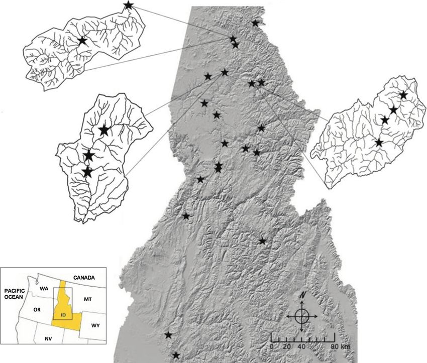
625Figure 1. Map of American dipper Cinclus mexicanus study reaches (n 26) used in this study and their distribution across Idaho, USA.
For watersheds with multiple study reaches, drainages are enlarged (as call-outs) and show the distribution of study reaches within the
watersheds.
zones, we conducted assessments of canopy coverage (%) rapid habitat assessment (IRHA), integrated the non-biotic
and riparian width (m) and completed a proper function- Idaho evaluation criteria into the Vermont assessment
ing condition (PFC) assessment (Barrett et al. 1998) along framework to provide a more quantitative protocol aimed
250 m centered around the nest. We estimated the percent- at capturing simplification of habitat diversity across the
age of canopy cover by walking the reach, using a spheri- entire reach (Barbour et al. 1999). We scored ten catego-
cal densiometer to estimate the degree of canopy extending ries (for each category, 0 represents worst condition and 20,
over the stream at three representative locations. To measure optimal condition) representing flow conditions, sedimenta-
the width of the riparian zone, we used a measuring tape to tion, habitat structure and complexity, bank condition, and
record the distance along three equidistantly spaced transects riparian vegetation and structure. When aggregated, these
on each side of the stream, running perpendicular to the individual scores yield an overall habitat evaluation ranging
stream channel to the farthest extent of the riparian zone as from 0 to 200.
determined by distinct changes in vegetation (Jackson and We conducted stream geomorphic assessments focus-
Sullivan 2009). The PFC is used to evaluate the ecological ing on both morphological characteristics and condition.
status and potential of a riparian area to dissipate stream Because dipper reaches in our study were typically homog-
energy associated with high flows. Each of seventeen con- enous in respect to channel morphology (Montgomery and
ditions in the PFC representing vegetation, landform/soils, Buffington 1997), we conducted geomorphic assessments
and hydrology are checked as yes, no, or N/A based on field along a 100 m reach around the nest site. We established
observations. Typically, these responses guide selection of a two lateral, representative transects (e.g. across the stream)
functional rating of the riparian zone. To use the PFC in and one longitudinal transect (e.g. bisecting the stream, run-
a more quantitative manner, we scored each riparian zone ning down its length). We then measured slope, bankfull
by calculating the percentage of ‘yes’ responses. Those ripar- width, and mean depth using a stadia rod, laser level, and
ian zones with the greatest percentage of ‘yes’ answers repre- measuring tape (Cianfrani et al. 2004). At each transect, we
sented riparian areas in highest condition. assessed percent embeddedness (degree to which fine sedi-
We developed a hybrid assessment of in-stream habi- ment surrounded cobbles) of 15 cobbles, and calculated the
tat quality based on both the Idaho small stream ecologi- mean percentage for an estimate of reach embeddedness.
cal assessment framework (Grafe 2002) and the Vermont Following Sullivan et al. (2006b), we evaluated the geomor-
rapid habitat assessment (RHA) protocols (VTDEC 2003). phic condition of each reach using rapid geomorphic assess-
Essentially, this hybrid, hereafter referred to as the Idaho ment (RGA) protocols (VTDEC 2003). We assigned a score
626from 0 (worst condition) to 20 (optimal condition) for each of Detailed land-cover categories were summed to produce
four geomorphic adjustment processes: channel degradation major land-use/cover classes: sparse (26–50% canopy cover),
(incision), channel aggradation, over-widened channel, and moderate (51–75% canopy cover), dense (76–100% canopy
change in planform (VTDEC 2003). We summed the scores cover), developed, evergreen forest, grassland-herbaceous,
of the four categories to form the composite RGA score. mixed deciduous forest, pasture/hay and cultivated crops,
We used ArcGIS 9.2 to derive drainage area (based on scrub/shrub, wetlands, and impervious surfaces 10%.
1:100 000 National Hydrography Dataset; USGS 1997) and Although we considered combining canopy coverage classes
Strahler’s (1952) stream order (based on 10-m digital eleva- into one category, we decided against this option due to the
tion data, INSIDE Idaho; UI 2009). potential ecological importance of threshold vegetation cov-
erage (Radford et al. 2005). For our roads layer, we accessed
the United States Geological Survey (USGS) National Map
Water quality and food abundance Seamless Server (USGS 2010).
Because our primary goal was to assess influences of the phys-
ical environment on dippers, we did not explicitly address Regional characteristics
water quality or food abundance in this study. However,
given the potential influences of water quality and food Regional characteristics focused on broad patterns related
abundance on dipper feeding, reproduction, and condition, to climate and geography. We designated the ecoregions of
we did address these factors through pre-study site screening each reach based on common ecosystem factors (e.g. geol-
and preliminary data. Although stream water quality across ogy, soils, vegetation, physiography, etc.) following the US
Idaho varies greatly, water quality concerns in mountain- Environmental Protection Agency’s Level III and IV classi-
ous regions where our sites were located are largely related fications (USEPA 2007). We used Garmin Rino 120 GPS
to erosion and sedimentation (Mahler and Van Steeter units to record the elevation of each study reach at its center
2002, Gravelle et al. 2009), which we captured through the (i.e. at the nest); we confirmed these readings using DEMs
RGA, RHA, PFC, and measurements of embeddedness. We generated using a GIS. We obtained temperature and pre-
screened all dipper reaches to ensure that no contaminant cipitation data from the Western Regional Climate Center
point-sources were present either within the reach or imme- (WRCC 2010) and from the National Climatic Data Center
diately upstream. (NESDIS 2010). For each study reach, we selected the clos-
Given the associations between stream acidity and est weather station, which was usually within the watershed.
Eurasian dipper C. cinclus abundance and reproductive For some very remote locations, the nearest station was
success (Ormerod et al. 1991, Tyler and Ormerod 1992), located in a neighboring watershed. We used daily precipita-
we surveyed pH at a random selection of half our dipper tion records to generate the amount of precipitation for each
streams. Twelve of the 13 territories had a pH of 7.5–8.3 year of the study (2005–2008) and for the breeding season
(circumneutral), while only one stream had a pH of 4.4 months (March–August) of each year. We averaged these
(acidic). Findings by other investigators gave us confidence values to calculate the breeding season mean precipitation
that additional variability in water chemistry among our (mm) and 2005–2008 mean precipitation (mm). Likewise,
sites would not be confounding factors in our analysis. For we used mean daily temperature readings to calculate the
example, Henny et al. (2005) reported high dipper repro- mean breeding season temperature (°C) for 2005–2008.
ductive success in spite of elevated MeHg concentrations
in Ephemeroptera, Plecoptera, and Trichoptera (EPT) lar-
Stable isotope analysis
vae, dipper eggs, and nestling feathers in tributaries of the
Willamette River, Oregon. Applications of stable isotopes allow for increased investi-
The high correlation between measures of aquatic mac- gation of trophic levels and diet studies and, therefore, are
roinvertebrates in the EPT orders and the in-stream habi- of particular use in describing food webs in aquatic ecosys-
tat assessments (EPT density and RHA score: r 0.686, tems (Collier et al. 2002, Hicks et al. 2005). Conventionally
p 0.0048; %EPT of total macroinvertebrate community expressed as d15N (‰) (see below), the ratio of 15N to 14N
and RHA score: r 0.572, p 0.0258) at a subset of 15 of typically exhibits a 3–4‰ enrichment with each trophic step,
the dipper territories (Sullivan unpubl.) enabled us to use and is commonly used to describe relative trophic position
the RHA as a coarse surrogate for food abundance and qual- (Kelly 2000). In our study, we used dipper blood to yield
ity. EPT larvae/nymphs are dominant in dipper diet during information related to the short term diet/assimilated foods:
the breeding season (Ealey 1977, Loegering and Anthony in the case of 15N, reflecting diet within 9–15 d (Hobson
1999). and Clark 1992, Bearhop et al. 2002). We interpreted dip-
per d15N signatures relative to baseline d15N values of stream
periphyton (i.e. the difference between dipper d15N and per-
Landscape characteristics iphyton d15N) to compare dipper trophic position across our
study reaches (Cabana and Rasmussen 1996).
We used the multi-resolution land characteristics consor- In the laboratory, we filtered and dried periphyton (60°C,
tium (MRLC) land-cover data layer based on 2001 national 48 h), followed by grinding in a ball mill and packing in tin
land cover data (NLCD; Vogelmann et al. 1998a, b) within capsules. Several samples per reach were combined to cre-
a geographic information system (GIS) to calculate land- ate composite periphyton samples for each reach. We dried
cover area percentages for each watershed (USGS 2009). all blood samples in a 60°C oven, and subsequently freeze
627dried (using a Labconco lyophilizer) and pulverized (using a priori models and sufficiently constrain the number of vari-
a ceramic mortar and pestle) all samples to ensure sample ables in each model (Riginos and Grace 2008, Paquette and
homogeneity. We packed and weighed (0.5–0.7 mg) samples Messier 2011).
in 4 6 mm tin capsules. Periphyton and replicate blood Structural models were carried out using the SEM soft-
samples were then analyzed at the Univ. of Washington ware Amos 17.0 (SPSS). Maximum likelihood procedures
Stable Isotope Core (Pullman, WA, USA). Values for 15N were used for estimation and to evaluate model goodness of
were calculated and reported using the standard delta (d) fit. Sequential application of c2 tests was used to determine
notation in parts per thousand (‰): which pathways to retain in the models. Amos also gener-
ates a full-model c2 value, which measures the degree of
dX [(Rsample/Rstandard) – 1] 1000 (1) discrepancy between the overall model and the data; when
p 0.05, the overall fit between the data and the final SE
where X is 15N and R is the corresponding ratio 15N:14N. model is considered acceptable. Once we had arrived at the
Typical analytical precision was 0.1‰ for d15N determination. model (or models) that we viewed to represent the most
likely relationships among the variables, we also generated
Bayesian estimates on the retained paths for confirmatory
Statistical analysis purposes, as these estimates do not rely on large-sample the-
ory (Lee 2007). A model whose retained path coefficients
To guide our analysis and inferences, we developed a con- have Bayesian 95% credible intervals that do not include
ceptual model that represented the general theoretical link- zero is considered supportive of a model derived from maxi-
ages without specifying statistical details (Grace 2006). This mum likelihood procedures.
model is presented in Supplementary material Appendix 1, The use of SEM to analyze spatially-explicit datasets is
Fig. A1. We then screened for potential spatial autocorrelation becoming increasingly common (Anderson et al. 2010,
among predictor and response variables using the Durbin– Paquette and Messier 2011) and may be advantageous
Watson d statistic (Connell et al. 1997). Subsequently, we in identifying both unique and synergistic contributions
analyzed our data using a sequential approach based on of predictor variables. Graham (2003) offered SEM as an
1) exploratory regression analysis and 2) structural equation alternative approach to multiple regression, in which the
modeling (SEM; Mitchell 1992, Grace and Pugesek 1998, functional nature of collinearities is considered. In the con-
Riginos and Grace 2008). text of this study, indirect paths (those connecting one or
For our exploratory analysis, we used principal compo- more predictor variables between spatial scales) indicate a
nent analysis (PCA) and multivariate regression to explore hierarchical and potentially synergistic influence on dipper
relationships between environmental features and dipper responses. Conversely, direct paths between predictor vari-
characteristics. Using environmental data gathered for each ables at regional, landscape, and/or local scales indicate inde-
spatial scale, we used PCA to generate axes that represented pendent influences on dipper responses. However, because it
our spatial scales of interest: regional, landscape, and local. is unlikely that SEM is fully robust against multicollinearity,
We then used the retained axes (eigenvalues 1; Rencher we did not did not include any highly correlated variables
1995) as predictor variables in mixed stepwise regressions. (r 0.8, Grewal et al. 2004) representing the same spatial
Dependent variables included dipper characteristics related scale in the same model; correlations of all variables between
to productivity (total no. eggs, total no. fledged, mean fledg- spatial scales were 0.6.
ling weight), d15N, and condition (mean female weight,
mean male weight). Given that multiple tests were per-
formed for each spatial scale, we ran a sequential Bonferroni Results
procedure to reduce type I errors (Holm 1979, Rice 1989).
Where necessary, data were transformed to meet assump- Dipper weight and reproduction varied across the study reaches
tions of multivariate normality. All analyses were performed (n 26), which represented a broad range of environmen-
using JMP 8.0 (SAS Inst.). For reference, results and addi- tal conditions (Table 1). On average, male dippers weighed
tional details from this exploratory analysis are presented approximately 4–5 g more than females during the breeding
in Supplementary material Appendix 2, Table A2.1–3 and months. The total number of eggs produced ranged from two
Appendix 3, Table A3.1. to nine, with a mean of five. Eighteen of the 26 pairs only pro-
SEM is a powerful tool in examining potential causal duced one clutch, and in 35% of nests the number of young
pathways among intercorrelated variables and exploring the successfully fledged was lower than the initial clutch size.
associations among variables while statistically controlling Across all reaches, dipper d15N signatures ranged from 5.0
for other model variables. SEM also generates estimates of to 10.2‰. Periphyton d15N values exhibited a narrow range
measurement error and suggests model improvements in (0.3–1.5‰) across the subset of study reaches from where it
evaluating alternative models (Bollen 1989). In conjunc- was collected. Dipper d15N signatures at these same reaches
tion with available published dipper-environmental rela- ranged from 5.0 to 8.7‰. Correcting for baseline periphyton
tionships, we used results from our exploratory analysis to d15N signatures yielded dipper d15N signatures ranging from
select the most promising explanatory variables to represent 4.4 to 7.5‰, resulting in a shift of only 0.5‰ in the range of
our conceptual parameters of interest in our SE models, original dipper d15N values (3.7‰, uncorrected; 3.2‰, cor-
represented by measures of 1) dipper productivity (total no. rected). Based on these results, we considered it reasonable to
fledged), 2) d15N, and 3) condition (mean male weight). use uncorrected dipper d15N values as surrogates for relative
In this way, our exploratory analysis enabled us to produce trophic position in an exploratory analysis.
628Table 1. Summary statistics of measures of regional, landscape, and local environmental characteristics, as well as measures of dipper
ecology from the 26 study reaches.
Minimum Median Maximum Mean SD
Regional variables
Elevation (m) 330.0 789.0 1176.0 758.4 217.6
Latitude (DD) 43.7 46.6 47.5 46.3 1.0
Precipitation (mm) – breeding season mean 0.8 1.1 2.7 1.5 0.3
Precipitation (mm) 2005–2008 mean 10.2 24.2 39.9 24.6 10.2
Temperature °C – breeding season mean 11.7 11.7 17.4 12.8 2.0
Level III ecoregion*
Level IV ecoregion*
Landscape variables
Sparse canopy cover (%) 2.9 8.9 24.9 10.3 5.6
Moderate canopy cover (%) 5.3 20.7 36.0 20.2 5.8
Dense canopy cover (%) 2.0 47.9 48.9 48.0 48.0
Developed (%) 0.0 0.0 2.8 0.3 0.7
Evergreen forest (%) 8.5 80.9 95.2 72.7 22.3
Grassland-herbaceous (%) 0.0 0.4 21.2 3.1 6.3
Imperviousness surfaces 10% (%) 0.0 0.2 13.2 0.8 2.6
Mixed deciduous forest (%) 0.0 0.0 0.6 0.1 0.1
No. stream crossings (by roads) per stream 0.0 36.5 61.8 35.0 17.9
length (no. 100 km1)
Pasture/hay and cultivated crops (%) 0.0 0.0 60.7 2.5 11.9
Road density (km 100 km2) 0.0 108.4 271.9 108.4 60.6
Shrub/scrub (%) 1.1 14.2 38.9 18.1 12.3
Wetlands (%) 0.0 0.1 1.3 0.2 0.3
Local variables
Bankfull depth(m) 0.5 1.0 2.3 1.1 0.4
Bankfull width (m) 5.7 13.7 31.5 14.8 6.9
Canopy (%) 0.0 16.3 50.0 17.9 11.8
Drainage area (km2 ) 21.8 124.6 1178.2 239.8 280.0
Embeddedness (%) 5.0 40.0 60.0 37.1 12.4
PFC (% yes) 12.5 62.5 100.0 56.9 26.4
RGA score 47.0 58.5 79.0 58.9 6.9
RHA score 102.0 128.5 194.0 131.5 22.2
Riparian width (m) 4.8 12.4 50.0 16.2 11.3
Slope (m m1) 0.004 0.015 0.122 0.024 0.023
Stream order 2.0 4.0 5.0 3.7 0.7
Dipper variables
Mean female weight (g) 45.9 58.6 67.0 56.5 5.9
Mean fledgling weight (g) 41.6 49.9 62.5 50.2 5.2
Mean male weight (g) 51.7 60.4 71.0 60.9 4.5
Total no. eggs 2.0 4.0 9.0 4.9 2.0
Total no. fledged 0.0 4.0 9.0 4.2 2.5
δ15N 5.0 6.6 10.2 6.4 1.3
*Level III and IV ecoregions were coded into the analysis as nominal variables.
Durbin–Watson tests indicated we were largely success- ent spatial scales were unique for each aspect of dipper
ful in avoiding spatial autocorrelation among our variables, ecology (Fig. 2). Productivity model 1 (c2 4.31,
with d 2 in the majority of cases (Durbin–Watson d 2.0 R2 0.58, p 0.89; Fig. 2a) was the most spatially inte-
indicates no pattern in variables across space, 1 indicates grative of all our models, depicting a multifaceted suite
clustering of variables in space) and with p 0.05 in all of interactions across all spatial scales in predicting the
cases except for grassland/herbaceous land cover (d 1.17, total no. fledged. Precipitation 2005–2008 (r 0.65) had
p 0.013). Given the low degree of autocorrelation of the strongest direct influence on the total no. fledged.
this variable and that it was incorporated into our explor- Dense canopy, in turn, was positively related to embed-
atory analysis as part of landscape principal components dedness, which was negatively related to total no. fledged.
(LandscapePCs, none of which were spatially autocorre- Bankfull width (r 0.29) also had a direct, positive effect
lated), we felt it was appropriate to leave this variable in the on the total no. fledged. Productivity model 2 (c2 5.13,
analysis. R2 0.45, p 0.40; Fig. 2b) was also a valid model in
our analysis, but not as strong as productivity model 1 in
Structural equation models predicting the total no. fledged (R2 0.58). Productivity
model 2 had no regional component, but both land
The final structural equation models provided evidence scape variables (dense canopy cover and shrub/scrub)
that the influences of environmental factors at differ- directly influenced the total no. fledged (r 0.34, 0.39;
629Figure 2. Structural equation modeling (SEM) analysis results for multiscalar characteristics influencing dipper productivity (a, b), d15N (c, d), and condition (e). Arrows represent direct and indirect influences (p 0.05). Numbers next to arrows are standardized regression coefficients, representing the relative strength of the given effect. The R2 values above the dipper response variable boxes represent the total variance explained by the model. Spatial scales are represented as follows:, regional, landscape; and local. n 26 for models 1–4 and n 22 for model 5. respectively). Riparian width shared an important associa- 2c). Regional characteristics, represented by measures of tion with geomorphic condition (r 0.48), which in turn precipitation and latitude, were the most influential vari- positively influenced total no. fledged (r 0.34). ables, accounting for the bulk of the variation observed Dipper d15N signatures, in contrast to number fledged, in d15N. The correlation between latitude and precipita- did not respond to variation in local characteristics tion 2005–2008 showed that these two regional metrics (nitrogen model 1; c2 0.61, R2 0.51, p 0.89; Fig. were linked. Breeding season precipitationexerted a direct, 630
Figure 2. Continued.
positive influence on d15N in nitrogen model 2 (c2 9.29, Discussion
R2 0.53, p 0.23; Fig. 2d). Grassland/herbaceous was an
important intermediary in both nitrogen models 1 and 2, In this study, we have examined several dipper ecological
positively influencing d15N in both cases. Nitrogen model responses to environmental characteristics at regional, land-
2 illustrated that moderate canopy cover may also represent scape, and local scales. Many have illustrated the hierarchical
a mechanistic link between latitude (r 0.46) and d15N influence of watershed characteristics on stream biota (Poff
(r 0.37). 1997); few have considered organisms that spatially integrate
Our condition model, represented by male weight riverine landscapes across their multiple dimensions (Fausch
(c2 2.79, R2 0.73, p 0.59; Fig. 2e), included breed- et al. 2002, Sullivan et al. 2007). Our results show that among
ing season precipitation and elevation as regional influences the physical environmental variables considered in this study,
on male weight. Breeding season precipitation exerted regional and landscape characteristics combined to exert the
a direct, positive influence on male weight (r 0.59), greatest influence, explaining patterns in dipper productiv-
whereas elevation was linked indirectly with male weight ity, d15N, and individual condition. Local characteristics
via pasture, hay, and cultivated crops (r 0.45). Pasture, of influence appear to be dominated by hydrogeomorphic
hay, and cultivated crops, in turn, positively influenced characteristics. Overall, we found that multiple facets of dip-
male weight (r 0.30). Road density appeared to act per ecology were influenced by factors that operated simulta-
independently on male weight (r 0.26). neously at different spatial scales. This information increases
Bayesian estimation procedures, used for small sam- our understanding of dipper-ecosystem linkages and of
ple sizes, confirmed that all paths retained in productiv- hierarchical relationships in watersheds.
ity model 1, productivity model 2, and nitrogen model 2 We considered multiple SE models for each dipper
had coefficients with 95% credible intervals that did not response variable, and have presented the strongest models
include zero. Nitrogen model 1 and the condition model for each of the three dipper measures representing our focal
had very slight deviations from zero but given the strength branches of dipper ecology–productivity, d15N, and indi-
of the other measures of model fit and their ecological rel- vidual condition. It is not our intention that these models
evance, we felt they represented valid models. represent the only possible environment–dipper trajectories,
631but rather that they present scenarios for which our data lend et al. 2004, 2006b, Sullivan and Watzin 2008). In a study in
the greatest support among the models considered. Overall, Vermont, USA, Sullivan et al. (2006a) showed that stream
in spite of detailed data representing many environmental channels undergoing geomorphic adjustment were negatively
features, direct regional-to-dipper and landscape-to-dipper associated with belted kingfisher Ceryle alcyon reproductive
pathways dominated SE models (Fig. 2). Across all models, measures. Vaughan et al. (2007) found that C. cinclus occu-
there were only three local-to-dipper pathways (productivity pancy was associated with multiple hydromorphological mea-
models 1 and 2, Fig. 2a, b). Among these, only productivity sures (e.g. cobble substrate, rocky channel, riffles) recorded by
model 1 (Fig. 2a) exhibited the full complement of interac- the United Kingdom’s Environmental Agency’s River Habitat
tions and influences across the three spatial scales. Survey (RHS). Price and Bock (1983) observed that heavy
siltation reduced dipper productivity, a result consistent with
our findings that increased embeddedness negatively influ-
Productivity enced dipper productivity.
Productivity model 2 (Fig. 2b) also included ripar-
Productivity, expressed by total no. fledged, was heavily ian width, an important predictor of in-stream condition
influenced by average precipitation over the study period, (Allan et al. 1997, Naiman and Décamps 1997, Frimpong
both directly (r 0.65) as well as indirectly via bankfull et al. 2005) and of considerable importance to both
width (r 0.38) (productivity model 1, Fig. 2a). Although migrant and resident birds (Saab 1999, Donovan et al.
our results indicate that greater amounts of precipitation 2002). Currently, the importance of riparian forests to dip-
may be favorable for dipper productivity, extreme precipi- pers is uncertain. Loegering and Anthony (2006) observed
tation events may reduce productivity due to higher flows, that 91% of dipper nest locations in their study area were
increased suspended sediment, and lower food availability, located where trees dominated both sides of the stream.
as observed by Price and Bock (1983) in Colorado, USA. Tyler and Ormerod (1994) observed a link between bank
Conversely, drought conditions might also be expected to tree cover and C. cinclus distribution, whereas Vaughan et
adversely affect dipper productivity through changes in water al. (2007) found no strong association with riparian tree
quality and macroinvertebrate communities (Finn et al. coverage. Our results provide evidence that riparian charac-
2009, Whitehead et al. 2009). During our study, variability teristics may be indirectly important to dippers by improv-
in precipitation, ranging only from 10.2 to 39.9 mm yr1, ing stream geomorphic condition (Fig. 2b).
was unlikely to capture potential dipper responses to extreme
precipitation shifts.
Differences in latitude, representing an approximate Nitrogen
450-km span between the northernmost and south-
ernmost study reaches, may play at least some role in Many investigations have greatly contributed to our knowl-
governing productivity (Fig. 2a), notably through indirect edge of stream food webs at the local scale (Schmid-Araya
effects of dense canopy coverage, and in turn, stream embed- et al. 2002, England and Rosemond 2004, Coat et al. 2009),
dedness. Although there is scant literature related to relation- yet there exists a current knowledge gap relating to the spa-
ships between land use and aquatic bird reproductive success tial scales of trophic dynamics in streams (Finlay et al. 2002).
in watersheds (Ormerod and Watkinson 2000, Mattson Nitrogen models 1 and 2 (Fig. 2c, d) highlight the importance
and Cooper 2006), evidence suggests that catchment for- of regional characteristics on dipper d15N signatures. d15N
est cover may explain significant variation in productivity signatures may reflect differences in the relative trophic posi-
of other aquatic taxa including algae, invertebrates, and fish tion of consumers, given comparable signals among stream
(Stephenson and Morin 2009). Dense canopy cover in our autotrophs (Post 2002), as in our study. The 5.7‰ range
study was heavily influenced by latitude, with greater cov- in dipper d15N values across our study reaches represents
erage of dense canopy at higher latitudes. Higher latitudes ∼1.5 to 2 trophic steps among sites (Kelly 2000). The posi-
also correlated with greater precipitation (Fig. 2a), which we tive influence of grassland-herbaceous and moderate canopy
speculate may lead to greater embeddedness in these streams cover on d15N signatures is consistent with the concept that
due to surface runoff. Catchment forest cover might be trophic links may increase in streams flowing through more
hypothesized to also influence nest predator abundance and open environments (Vannote et al. 1980). For instance,
activity (Chalfoun et al. 2002, Mattson and Cooper 2006), Gothe et al. (2009) observed that both basal resources and
but predation rates on dipper nests in this and other studies aquatic invertebrate consumers were 15N-enriched in clear-
(Morrissey 2004) are relatively low compared to nest preda- cut compared to old-growth streams. However, recent find-
tion rates for many passerine species. ings by Sabo et al. (2010) suggest that increases in food chain
In our study, factors of influence at the local scale (Fig. 2a, length may be governed by increases in drainage area, with
b) were largely related to hydrogeomorphic variables (e.g. geo- hydrologic variability acting as the underlying mechanism.
morphic condition, embeddedness, bankfull width). Study Although this pattern was represented by a trend in our raw
streams with low geomorphic conditions exhibited significant data, the relationship was not sufficiently strong to emerge
sediment accumulation, eroding banks, widened channels in our SE models, likely because breeding dippers are con-
with reduced heterogeneity in flow patterns, and other charac- strained to high-gradient, smaller stream systems. Given that
teristics suggestive of channel adjustment and homogenization dippers represent top predators in these systems, our results
of habitat. Other investigators have also documented associa- contribute to the current understanding of drivers of food
tions between stream geomorphic adjustment, habitat qual- chain length, and support the potentially important role of
ity, and multiple aquatic taxa (Walters et al. 2003, Sullivan spatial effects (Sabo et al. 2009).
632Condition Regional variables are not commonly considered in water-
shed studies, but as human activities continue to expand
Body mass of birds has often been used as a measure of habi- their reach, it will be increasingly important to incorporate
tat quality (Johnson et al. 2006, Smith et al. 2010) and can broad-scale attributes. For example, our understanding of the
be influenced by a number of factors, including latitude, food impacts of climate change on aquatic organisms is hobbled by
availability, habitat type, species-specific traits, and gender- the difficulty in gathering data at and assessing large spatial
specific roles during breeding (Moreno 1989). The condi- scales. Changes in temperature and precipitation, however,
tion model (Fig. 2e) explained the majority of the variation may alter the distribution (Peterson et al. 2002, McKenney
observed in male weight, indicating that by and large, male et al. 2007) and abundance (McLaughlin et al. 2002) of
condition during the breeding season is controlled by factors many species. For instance, rainfall extremes influenced
operating beyond the local scale. Breeding season precipita- reproduction of the Louisiana waterthrush Seiurus motacilla,
tion again emerged as an influential factor, signifying that a riparian obligate species (Mattsson and Cooper 2009), and
climatic variability is expressed at the individual as well as these authors suggest that rainfall patterns are likely to have
population levels (Saether et al. 2004). variable species-specific effects on riparian breeding birds.
At the landscape scale, human activities in the form of In our study, dippers responded to precipitation measured
agricultural and transportation infrastructure influenced at two temporal scales, indicating that both immediate and
male weight. Whereas elevation was negatively associated longer-term precipitation patterns may drive the demograph-
with the percentage of agriculture, road density emerged as a ics of dipper populations. Likewise, Chiu et al. (2008) found
factor independent from regional characteristics. Our results strong associations between flood magnitude and brown
support existing literature related to the detrimental ecologi- dippers Cinclus pallasii and proposed that influences of flood-
cal impacts of roads (Angermeier et al. 2004, Wheeler et al. ing be considered when using dippers as bioindicators.
2005). For dippers, local populations can be limited by the There are some important caveats regarding this study.
lack of suitable nesting sites (Loegering and Anthony 2006), Firstly, the covariation of anthropogenic and natural landscape
and breeding pairs frequently nest under bridges, where attributes can often lead to an overestimation of the influence
localized changes in channel geomorphology and streams of land use (Allan 2004). Although we have identified land-
sedimentation may exacerbate the effects of roads. In our use attributes of potential influence on dipper ecology, our pri-
study, road density appeared to negatively influence male mary goal was to use these attributes to represent the impact
weight, but not female weight, emphasizing that males and of factors at the landscape spatial scale. Secondly, our study
females may respond differently to factors during the breed- focused on physical environmental characteristics. Additional
ing season. For instance, Morrissey et al. (2010) observed that factors that would account for unexplained variance include
egg-laying females fed at a higher trophic level than males more detailed data relating to food resources (Morrissey
by consuming more fish in streams in British Columbia, et al. 2010), water quality (Ormerod and Tyler 1993, Brewin
Canada. Because female dippers are solely responsible for et al. 1998), and competition for territory and nesting sites
incubating eggs and are primarily responsible for feeding (Loegering and Anthony 2006, Gillis et al. 2008).
of nestlings in the early stages of hatchling development Our study provides a perspective on species-ecosystem
(Kingery 1996), it is likely that females remain closer to the relationships based on multiple facets of dipper ecology, a
nest. Conversely, male condition, reflecting activity across broad array of environmental characteristics, and multiple
the full length of the breeding territory, might be expected spatial scales. The potential of dippers as bioindicators of
to integrate landscape-level habitat characteristics. stream condition and water quality (Price and Bock 1983,
Strom et al. 2002, Morrissey et al. 2004) suggests that our
results may extend beyond American dipper ecology and, to
Conclusions an extent, represent broader stream-watershed associations.
In particular, the influences of environmental characteristics
Increased understanding of spatial patterns in stream eco- at multiple spatial scales indicate that dippers may spatially
systems (Fausch et al. 2002, Vaughn 2010) highlights integrate watershed landscapes through their productiv-
the need for empirical research that addresses species- ity, feeding, and individual condition (Sullivan et al. 2007,
ecosystem linkages across spatial scales (Lowe et al. 2006). Sullivan and Vierling 2009). As we continue to consider
In the present study, we have shown that both direct and stream-riparian ecosystems from a landscape perspective,
indirect effects related to multiscalar environmental char- we propose it will be beneficial to consider organisms with
acteristics influenced multiple aspects of dipper ecol- potential to represent both the riverscape (Fausch et al. 2002,
ogy. Our SE models (Fig. 2) highlighted the prevalence Sullivan et al. 2007) and spatial components of watersheds
of regional-to-dipper and landscape-to-dipper relation- in ways that other, more traditional aquatic biota, may not.
ships, with local factors often by-passed. Precipitation, Given the heavy influence of regional and landscape charac-
for instance, drove patterns in dipper productivity, d15N, teristics on dippers, our results also advocate for increased
and individual condition. Our results offer evidence that incorporation of large-scale features in both the develop-
although stream-watershed habitats may be spatially- ment and application of stream-riparian habitat assessment
nested, the pathways influencing American dippers may and conservation protocols.
not always conform to hierarchical spatial relationships
(Burcher et al. 2007). Investigating if these patterns are Acknowledgements – We are grateful to Ryan Mann and Matthew
unique to dippers or are shared by other aquatic biota Mason for their assistance in the field and lab. Chi Vuong and
offers an intriguing line of future research. Adam Kautza provided valuable assistance with the remote sensing
633and GIS work. We also extend thanks to Breeanne Jackson, John Coat, S. et al. 2009. Trophic relationships in a tropical stream food
Cassinelli, Giancarlo Sadoti, and Kath Strickler for their help. web assessed by stable isotope analysis. – Freshw. Biol. 54:
Research was funded by the Mountaineers Foundation (SMPS), 1028–1041.
US Forest Service Collaborative Working Forest Initiative (SMPS), Collier, K. J. et al. 2002. A stable isotope study of linkages between
NSF Division of Ecological Biology 0534815 (KTV), and the stream and terrestrial food webs through spider predation.
Univ. Idaho (SMPS and KTV). – Freshw. Biol. 47: 1651–1659.
Connell, J. H. et al. 1997. A 30-year study of coral abundance,
recruitment, and disturbance at several scales in space and time.
– Ecol. Monogr. 67: 461–488.
References Donovan, T. M. et al. 2002. Priority research needs for the conser-
vation of Neotropical migrant landbirds. – J. Field Ornithol.
Allan, J. D. 2004. Landscapes and riverscapes: the influence of land 73: 329–339.
use on stream ecosystems. – Annu. Rev. Ecol. Evol. Syst. 35: Ealey, D. M. 1977. Aspects of the ecology and behaviour of a
257–284. breeding population of dippers (Cinclus mexicanus: Passeri-
Allan, J. D. and Johnson, L. B. 1997. Catchment-scale analysis of formes) in southern Alberta. – Univ. of Alberta.
aquatic ecosystems. – Freshw. Biol. 37: 107–111. England, L. E. and Rosemond, A. D. 2004. Small reductions in
Allan, J. D. et al. 1997. The influence of catchment land use on forest cover weaken terrestrial-aquatic linkages in headwater
stream integrity across multiple spatial scales. – Freshw. Biol. streams. – Freshw. Biol. 49: 721–734.
37: 149–161. Fausch, K. D. et al. 2002. Landscapes to riverscapes: bridging the
Allen, T. F. and Hoekstra, T. W. 1992. Towards a unified ecology. gap between research and conservation of stream fishes. – Bio-
– Columbia Univ. Press. science 52: 483–498.
Anderson, T. M. et al. 2010. Landscape-scale analyses suggest both Finlay, J. C. et al. 2002. Spatial scales of carbon flow in a river food
nutrient and antipredator advantages to Serengeti herbivore web. – Ecology 83: 1845–1859.
hotspots. – Ecology 91: 1519–1529. Finn, M. A. et al. 2009. Ecological responses to artificial drought
Angermeier, P. L. et al. 2004. A conceptual framework for assessing in two Australian rivers with differing water extraction. – Fun-
impacts of roads on aquatic biota. – Fisheries 29: 19–29. dam. Appl. Limnol. 175: 231–248.
Ardia, D. R. 2005. Tree swallows trade off immune function and Foster, D. et al. 2003. The importance of land-use legacies to ecol-
reproductive effort differently across their range. – Ecology 86: ogy and conservation. – Bioscience 53: 77–88.
2040–2046. Frimpong, E. A. et al. 2005. Spatial-scale effects on relative impor-
Barbour, M. T. et al. 1999. Rapid bioassessment protocols for use tances of physical habitat predictors of stream health. – Envi-
in streams and wadeable rivers: periphyton, benthic macroin- ron. Manage. 36: 899–917.
vertebrates and fish. – EPA 841-B-99-002, US Environmental Frissell, C. A. et al. 1986. A hierarchical framework for stream
Protection Agency. habitat classification: viewing streams in a watershed context.
Barrett, H. et al. 1998. Riparian area management: process for – Environ. Manage. 10: 199–214.
assessing proper functioning condition. – Tech. Ref. 1737-9, Gillis, E. A. et al. 2008. Life history correlates of alternative migra-
US Dept of the Interior, Bureau of Land Management. tory strategies in American dippers. – Ecology 89: 1687–1695.
Baxter, C. V. et al. 2005. Tangled webs: reciprocal flows of inver- Gothe, E. et al. 2009. Forestry affects food webs in northern Swed-
tebrate prey link streams and riparian zones. – Freshw. Biol. ish coastal streams. – Fundam. Appl. Limnol. 175: 281–294.
50: 201–220. Grace, J. B. 2006. Structural equation modeling and the study of
Bearhop, S. et al. 2002. Factors that influence assimilation rates natural systems. – Cambridge Univ. Press.
and fractionation of nitrogen and carbon stable isotopes in Grace, J. B. and Pugesek, B. H. 1998. On the use of path analysis
avian blood and feathers. – Physiol. Biochem. Zool. 75: and related procedures for the investigation of ecological prob-
451–458. lems. – Am. Nat. 152: 151–159.
Ben-David, M. et al. 1998. Fertilization of terrestrial vegetation by Grafe, C. S. 2002. Idaho small stream ecological assessment frame-
spawning Pacific salmon: the role of flooding and predator work: an integrated approach. – Idaho Dept of Environmental
activity. – Oikos 83: 47–55. Quality.
Bollen, K. A. 1989. Structural equations with latent variables. Graham, M. H. 2003. Confronting multicollinearity in ecological
– Wiley. multiple regression. – Ecology 84: 2809–2815.
Brewin, P. A. et al. 1998. River habitat surveys and biodiversity in Gravelle, J. A. et al. 2009. Effects of timber harvest on aquatic
acid-sensitive rivers. – Aquat. Conserv. 8: 501–514. macroinvertebrate community composition in a northern
Brown, J. H. 1995. Macroecology. – Univ. of Chicago Press. Idaho watershed. – For. Sci. 55: 352–366.
Burcher, C. L. et al. 2007. The land-cover cascade: relationships Grewal, R. et al. 2004. Multicollinearity and measurement error in
coupling land and water. – Ecology 88: 228–242. structural equation modeling. – Marketing Sci. 23: 519–529.
Cabana, G. and Rasmussen, J. B. 1996. Comparison of aquatic Guegan, J. F. et al. 1998. Energy availability and habitat heterogeneity
food chains using nitrogen isotopes. – Proc. Natl Acad. Sci. predict global riverine fish diversity. – Nature 391: 382–384.
USA 93: 10844–10847. Harding, J. S. et al. 1998. Stream biodiversity: the ghost of land
Camilleri, S. et al. 2010. The interaction between land use and catch- use past. – Proc. Natl Acad. Sci. USA 95: 14843–14847.
ment physiognomy: understanding avifaunal patterns of the Hatch, M. I. and Smith, R. J. 2010. Repeatability of hematocrits and
Murray-Darling Basin, Australia. – J. Biogeogr. 37: 293–304. body mass of gray catbirds. – J. Field Ornithol. 81: 64–70.
Chalfoun, A. D. et al. 2002. Nest predators and fragmentation: a Henny, C. J. et al. 2005. Assessing mercury exposure and effects
review and meta-analysis. – Conserv. Biol. 16: 306–318. to American dippers in headwater streams near mining sites.
Chiu, M. C. et al. 2008. Effects of flooding on avian top-predators – Ecotoxicology 14: 709–725.
and their invertebrate prey in a monsoonal Taiwan stream. Herrera, L. G. et al. 2005. Quantifying differential responses to
– Freshw. Biol. 53: 1335–1344. fruit abundance by two rainforest birds using long-term iso-
Cianfrani, C. M. et al. 2004. Evaluating aquatic habitat quality topic monitoring. – Auk 122: 783–792.
using channel morphology and watershed scale modeling tech- Hicks, J. H. et al. 2005. Marine-derived nitrogen and carbon in
niques. – World Water and Environment Resources Congress, freshwater-riparian food webs of the Copper River Delta,
American Society of Civil Engineers. southcentral Alaska. – Oecologia 144: 558–569.
634Hobson, K. A. and Clark, R. G. 1992. Assessing avian diets using Morrissey, C. A. 2004. Effect of altitudinal migration within a
stable isotopes: turnover of C-13 in tissues. – Condor 94: watershed on the reproductive success of American dippers.
181–188. – Can. J. Zool. 82: 800–807.
Holm, S. 1979. A simple sequentially rejective multiple test pro- Morrissey, C. A. et al. 2004. Linking contaminant profiles to the
cedure. – Scand. J. Stat. 6: 65–70. diet and breeding location of American dippers using stable
Hubbel, S. P. 2001. The unified theory of biodiversity and bioge- isotopes. – J. Appl. Ecol. 41: 502–512.
ography. – Princeton Univ. Press. Morrissey, C. A. et al. 2010. Diet shifts during egg laying: implica-
Hynes, H. B. N. 1975. Edgardo Baldi Memorial Lecture. The tions for measuring contaminants in bird eggs. – Environ.
stream and its valley. – Verh. Int. Ver. Theor. Angew. Limnol. Pollut. 158: 447–454.
19: 1–15. Naiman, R. J. and Décamps, H. 1997. The ecology of interfaces:
Imhof, J. G. et al. 1996. A hierarchical evaluation system for char- riparian zones. – Annu. Rev. Ecol. Syst. 28: 621–658.
acterizing watershed ecosystems for fish habitat. – Can. J. Fish. Nakano, S. and Murakami, M. 2001. Reciprocal subsidies: dynamic
Aquat. Sci. 53: 312–326. interdependence between terrestrial and aquatic food webs.
Jackson, B. K. and Sullivan, S. M. P. 2009. Influence of wildfire – Proc. Natl Acad. Sci. USA 98: 166–170.
severity on riparian plant community heterogeneity in an NESDIS 2010. Online climate data directory website. – National
Idaho, USA wilderness. – For. Ecol. Manage. 259: 24–32. Environmental Satellite, Data, and Information Service (NES-
Johnson, L. B. et al. 1997. Landscape influences on water DIS), http://lwf.ncdc.noaa.gov/oa/climate/climatedata.html.
chemistry in midwestern stream ecosystems. – Freshw. Biol. 37: Ormerod, S. J. 1985. The diet of breeding dippers (Cinclus cinclus)
193–208. and their nestlings in the catchment of the River Wye, mid-
Johnson, M. D. et al. 2006. Assessing habitat quality for a migra- Wales; a preliminary study by faecal analysis. – Ibis 127: 316–
tory songbird wintering in natural and agricultural habitats. 331.
– Conserv. Biol. 20: 1433–1444. Ormerod, S. J. and Tyler, S. J. 1987. Dippers (Cinclus cinclus) and
Kelly, J. F. 2000. Stable isotopes of carbon and nitrogen in the grey wagtails (Motacilla cinera) as indicators of stream aciditity
study of avian and mammalian trophic ecology. – Can. J. Zool. in upland Wales. – In: Diamond, A. W. et al. (eds), The value
78: 1–27. of birds. International Council for Bird Preservation Technical
Kingery, H. E. 1996. American dipper (Cinclus mexicanus). – In: Pubication 6, International Council for Bird Preservation, pp.
Poole, A. and Gill, F. (eds), The birds of North America. The 191–208.
Academy of Natural Sciences and The American Ornithologists Ormerod, S. J. and Tyler, S. J. 1993. Birds as indicators of changes
Union. in water quality. – In: Furness, R. W. and Greenwood, J. J. D.
Lee, S. Y. 2007. Structural equation modeling: a Bayesian approach. (eds), Birds as monitors of environmental change. Chapman
– Wiley. and Hall, pp. 179–216.
Leu, M. et al. 2008. The human footprint in the West: a large- Ormerod, S. J. and Watkinson, A. R. 2000. Large-scale ecology
scale analysis of anthropogenic impacts. – Ecol. Appl. 18: and hydrology: an introductory perspective from the editors of
1119–1139. the Journal of Applied Ecology. – J. Appl. Ecol. 37: 1–5.
Loegering, J. P. and Anthony, R. G. 1999. Distribution, abun- Ormerod, S. J. et al. 1991. The ecology of dippers Cinclus cinclus
dance, and habitat associations of riparian-obligate and -associ- in relation to stream acidity in upland Wales: breeding per-
ated birds in the Oregon Coast Range. – Northwest. Nat. 73: formance, calcium physiology and nestling growth. – J. Appl.
168–185. Ecol. 28: 419–433.
Loegering, J. P. and Anthony, R. G. 2006. Nest-site selection and Paquette, A. and Messier, C. 2011. The effect of biodiversity on
productivity of American dippers in the Oregon Coast Range. tree productivity: from temperate to boreal forests. – Global
– Wilson J. Ornithol. 118: 281–294. Ecol. Biogeogr. 20: 170–180.
Logie, J. W. et al. 1996. Biological significance of UK critical load Peterson, A. T. et al. 2002. Future projections for Mexican faunas
exceedance estimates for flowing waters: assessments of dipper under global climate change scenarios. – Nature 416: 626–629.
Cinclus cinclus populations in Scotland. – J. Appl. Ecol. 33: Poff, N. L. 1997. Landscape filters and species traits: towards
1065–1076. mechanistic understanding and prediction in stream ecology.
Lowe, W. H. et al. 2006. Linking scales in stream ecology. – Bio- – J. North Am. Benthol. Soc. 16: 391–409.
science 56: 591–597. Post, D. 2002. Using stable isotopes to estimate trophic position:
Mahler, R. L. and Van Steeter, M. M. 2002. Idaho’s water resource. models, methods, and assumptions. – Ecology 83: 703–718.
– Current Information Series no. 887, Univ. of Idaho. Price, F. E. and Bock, C. E. 1983. Population ecology of the dipper
Mattson, B. J. and Cooper, R. J. 2006. Louisiana waterthrushes (Cinclus mexicanus) in the Front Range of Colorado. – Studies
(Seiurus motacilla) and habitat assessments as cost-effective in Avian Biology no. 7, Cooper Ornithological Society.
indicators of instream biotic integrity. – Freshw. Biol. 51: Radford, J. Q. et al. 2005. Landscape-level thresholds of habitat
1941–1958. cover for woodland-dependent birds. – Biol. Conserv. 124:
Mattsson, B. J. and Cooper, R. J. 2009. Multiscale analysis of the 317–337.
effects of rainfall extremes on reproduction by an obligate ripar- Rencher, A. C. 1995. Methods of multivariate analysis. – Wiley.
ian bird in urban and rural landscapes. – Auk 126: 64–76. Rice, W. R. 1989. Analyzing tables of statistical tests. – Evolution
McKenney, D. W. et al. 2007. Potential impacts of climate change 43: 223–225.
on the distribution of North American trees. – Bioscience 57: Richards, C. et al. 1997. Catchment and reach-scale properties as
939–948. indicators of macroinvertebrate species traits. – Freshw. Biol.
McLaughlin, J. F. et al. 2002. Climate change hastens population 37: 219–230.
extinctions. – Proc. Natl Acad. Sci. USA 99: 6070–6074. Riginos, C. and Grace, J. B.. 2008. Savanna tree density, herbiv-
Mitchell, R. J. 1992. Testing evolutionary and ecological hypoth- ores, and the herbaceous community: bottom-up vs top-down
eses using path-analysis and structural equation modeling. effects. – Ecology 89: 2228–2238.
– Funct. Ecol. 6: 123–129. Roth, N. E. et al. 1996. Landscape influences on stream biotic
Montgomery, D. R. and Buffington, J. M. 1997. Channel-reach integrity assessed at multiple spatial scales. – Landscape Ecol.
morphology in mountain drainage basins. – Geol. Soc. Am. 11: 141–156.
Bull. 109: 596–611. Saab, V. 1999. Importance of spatial scale to habitat use by breed-
Moreno, J. 1989. Strategies of mass change in breeding birds. ing birds in riparian forests: a hierarchical analysis. – Ecol.
– Biol. J. Linn. Soc. 37: 297–310. Appl. 9: 135–151.
635You can also read