Spatial Assessment of the Association between Long-Term Exposure to Environmental Factors and the Occurrence of Amyotrophic Lateral Sclerosis in ...
←
→
Page content transcription
If your browser does not render page correctly, please read the page content below
Methods in Neuroepidemiology

                                                        Neuroepidemiology 2018;51:33–49                                          Received: February 17, 2018
                                                                                                                                 Accepted: April 27, 2018
                                                        DOI: 10.1159/000489664                                                   Published online: May 31, 2018

Spatial Assessment of the Association between
Long-Term Exposure to Environmental Factors
and the Occurrence of Amyotrophic Lateral
Sclerosis in Catalonia, Spain: A Population-Based
Nested Case-Control Study
Mònica Povedano a Marc Saez b, c Juan-Antonio Martínez-Matos a
Maria Antònia Barceló a–c
a FunctionalMotoneurona Unit (UFMNA), Bellvitge Biomedical Research Institute (IDIBELL), L’Hospitalet de
Llobregat, Barcelona, Spain; b Research Group on Statistics, Econometrics and Health (GRECS), University of Girona,
Girona, Spain; c CIBER of Epidemiology and Public Health (CIBERESP), Madrid, Spain

Keywords                                                                    served confounders. Results: We have found some spatial
Amyotrophic lateral sclerosis · Environmental                               clusters of ALS. The results from the multivariate model sug-
variables · Pesticides · Air pollutants · Unobserved                        gest that these clusters could be related to some of the en-
confounding · Spatial dependence                                            vironmental variables, in particular agricultural chemicals.
                                                                            In addition, in high-risk clusters, besides corresponding to
                                                                            agricultural areas, key road infrastructures with a high den-
Abstract                                                                    sity of traffic are also located. Conclusion: Our results indi-
Background: It is believed that an interaction between ge-                  cate that some environmental factors, in particular those as-
netic and non-genetic factors may be involved in the devel-                 sociated with exposure to pesticides and air pollutants as a
opment of amyotrophic lateral sclerosis (ALS). With the ex-                 result of urban traffic, could be associated with the occur-
ception of exposure to agricultural chemicals like pesticides,              rence of ALS.                              © 2018 S. Karger AG, Basel
evidence of an association between environmental risk fac-
tors and ALS is inconsistent. Our objective here was to inves-
tigate the association between long-term exposure to envi-
ronmental factors and the occurrence of ALS in Catalonia,                       Introduction
Spain, and to provide evidence that spatial clusters of ALS
related to these environmental factors exist. Methods: We                      Amyotrophic lateral sclerosis (ALS) is a rapidly pro-
carried out a nested case-control study constructed from a                  gressing, neurodegenerative disease characterized by a
retrospective population-based cohort, covering the entire                  progressive loss of upper and lower motor neurons that
region. Environmental variables were the explanatory vari-                  leads to muscular atrophy, paralysis and patient death,
ables of interest. We controlled for both observed and unob-                usually due to respiratory failure [1–4]. Different pheno-

                           © 2018 S. Karger AG, Basel                       Maria Antònia Barceló, PhD
                                                                            Research Group on Statistics, Econometrics and Health (GRECS) and CIBER of
                                                                            Epidemiology and Public Health (CIBERESP)
E-Mail karger@karger.com
                                                                            University of Girona, Carrer de la Universitat de Girona 10
www.karger.com/ned                                                          Campus de Montilivi, ES–17003 Girona (Spain), E-Mail antonia.barcelo @ udg.edu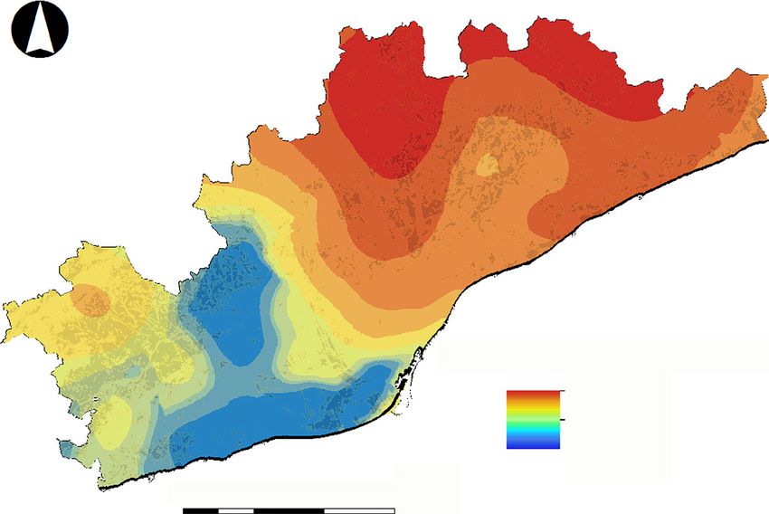
types and presentations of ALS have been identified and lower than in Europe. The ALS standardized incidence
are defined by where the symptoms of the disease first is 0.83 per 100,000 persons/years (95% CI 0.42–1.24) for
appear (spinal, bulbar, flail leg, flail arm, pyramidal or re- Eastern Asia and 0.73 per 100,000 persons/years (95%
spiratory), by whether the upper or lower motor neuron CI 0.58–0.89) for Southern Asia [10]. However, for the
is most affected (primary lateral sclerosis, progressive same period in Japan, the ALS incidence was estimated
muscular atrophy and classic ALS) and by the rate the equal to 2.2 per 100,000 persons/years [13]. The preva-
disease progresses (fast or slow). The overriding impor- lence of ALS has been estimated to be between 5 [14]
tance of these different phenotypes is in their prognosis and 5.4 per 100,000 inhabitants [9]. Geographic vari-
because some are less incapacitating and spread more ability also occurs. The highest figures are reported for
slowly than others and, unfortunately, for the others the Japan: 9.9 per 100,000 inhabitants in 2013 [13], practi-
prognosis is worse for the problems highlighted [5, 6]. cally twice as many as in the United States (3.9 per
Spinal and bulbar phenotypes account for 42.0 and 33.5%, 100,000 inhabitants in 2010–2011 [13], 4.3 in 2013 [15])
respectively, of the total cases of ALS, while the flail leg and Europe (4.06 per 100,000 inhabitants in western
phenotype accounts for 8.5% of all cases, the flail arm Europe [5]), both with fairly similar prevalence. Pradas
6.5%, pyramidal 5% and respiratory phenotype 4.5% [5, et al. [12] estimate a prevalence of 5.4 per 100,000 inhab-
6]. Genetic mutations do not entirely explain this hetero- itants for Catalonia, Spain.
geneity because the same mutation can be associated with Both in terms of the prevalence and incidence of ALS,
a large variability of ALS phenotypes. The dominantly in- heterogeneity also occurs with other variables such as
herited familial ALS, for which heredity is mainly autoso- sex and age. The incidence for men is between 1.3 and
mal dominant, only accounts for 10% of all ALS patients. 1.5 higher than that of women [15, 10, 12]. ALS is rare
Sporadic ALS has no apparent heritability and is the most before the age of 40 years, with the mean age at onset
common form of ALS. Although considerable progress ranging from 58 to 63 years for the sporadic form and
has been made in understanding the genetics of familial 40 to 60 years for the familial form [9]. There is very
ALS, the underlying causes of sporadic ALS remain un- little variation between the phenotypes [5, 6]. Subse-
known [7, 8]. So far, the only recognized ALS risk factors quent to the age of onset, the incidence of ALS increas-
are advanced age, being male and having a family history es and peaks after 60 years of age. Chiò et al. [5] found
of ALS [9]. that the incidence of ALS reaches its maximum from
In a very recent meta-analysis, which included 825 60 to 75 years of age. However, in the Cima study,
million person-years of follow-up and covered 45 geo- this maximum occurs from 65 to 74 years of age [16],
graphical areas in 11 sub-continents, Marin et al. [10], while in several studies in Nova Scotia, Canada, from 70
estimate the overall worldwide crude incidence of ALS to 79 years old [17].
equal to 1.75 per 100,000 persons/years of follow-up The heterogeneity and prevalence in the incidence of
(95% CI 1.55–1.96) with a standardized incidence of ALS may be a consequence of different diagnostic crite-
1.68 (95% CI 1.50–1.85). However, the geographical dis- ria, clinical practices and ways of recording cases. How-
tribution of ALS incidence is very heterogeneous. The ever, an important part of the heterogeneity can be at-
incidence of ALS in Europe has been estimated at around tributed to the interrelationship between genetic and
2–4 cases per 100,000 person/years [8]. This estimate is non-genetic factors [8, 18–23]. These non-genetic fac-
somewhat smaller in northern Europe where ALS stan- tors may include variables related to lifestyle (smoking,
dardized incidence is 1.89 per 100,000 persons/years consumption of antioxidants, physical exercise and
(95% CI 1.46–2.3) [10], although it is found to be high- body mass index), medical conditions (head injury,
er in western Europe. In a systematic review of popula- metabolic diseases, cancer and inflammatory diseases)
tion-based observational studies, including 37 articles, and work and environmental related exposure
Chiò et al. [5] estimated the incidence in western Europe (β-methylamino-L-alanine, viral infections, electromag-
for the period 1995–2011 as 5.40 per 100,000 and 4.70 netic fields, metals and pesticides) [20, 22]. However,
per 100,000 in 2012. In Spain, Santurtún et al. [11] the systematic evidence of the association between envi-
found an annual incidence ranging from 1 to 3 cases ronmental risk factors and the occurrence of ALS, be-
per 100,000 inhabitants in 2013, while for the same year, sides being very limited, is inadequate or insufficient.
Pradas et al. [12] estimated an annual incidence of We present, in decreasing order of the number of sys-
1.4 per 100,000 inhabitants in the Catalonia region tematic revisions, exposure to agricultural chemical
(north-eastern Spain). In Asia, the incidence is much products (i.e., pesticides) [18, 20–25], metals [21–26],
34 Neuroepidemiology 2018;51:33–49 Povedano/Saez/Martínez-Matos/Barceló
DOI: 10.1159/000489664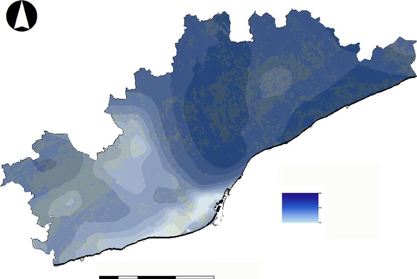
β-methylamino-L-alanine [18, 20–22] and electromag-            exposure to lead, with a pooled odds ratio of 1.81 (95%
netic fields [22].                                             CI 1.39–2.36). Santurtún et al. [11] found higher mortal-
   Comparatively, there is much more evidence on the           ity ratios for people older than 65 years in the provinces
association with ALS to the exposure to pesticides. In a       of northern Spain. There was a significant association
systematic review of 448 articles on the association be-       between their mortality from motor neuron diseases
tween pesticide exposure and human diseases, Mostafa-          and higher levels of lead in the air, suggesting that envi-
lou and Abdollahi [25] found 18 studies, 15 case-control       ronmental exposures had an important role to play. Two
and 3 cohorts assessing the relationship between pesti-        epidemiological surveys have found a higher incidence
cide exposure and ALS incidence. Ten of the 15 case-           of ALS in regions with high concentrations of selenium
control studies found an association between exposure to       in animal farms [42] and in well water [43]. With re-
pesticides and the occurrence of ALS, with the odds ra-        gards to iron, Hozumi et al. [44] found ALS patients
tios between 1.1 and 6.9 [27–36]. Kang et al. [24], from a     have higher cerebrospinal fluid iron concentrations. In
meta-analysis of 19 case-control and 3 cohort studies,         addition, a very recent meta-analysis including 6 case-
also found an association between the risk of ALS and          control studies found an association between elevated
pesticide exposure, (OR 1.44; 95% CI 1.22–1.70) and            serum ferritin levels and ALS [45]. Exposure to mercury
with farming (as an occupation, OR 1.42; 95% CI 1.17–          may be linked to the aetiology of ALS [46, 47]. A case in
1.73). They did not, however, find an association be-          point is the cluster located in a small fishing village next
tween the risk of ALS and exposure to rural environ-           to Lake Michigan, the United States, where the fish had
ments [24]. In an occupational context and using a meta-       high levels of mercury [48]. The association of risk to
analysis of 8 studies [37], Kamel et al. [37] provided         ALS and the exposure to manganese is inconsistent. In
evidence of the association between occupational expo-         fact, only 2 studies found a significantly higher concen-
sure to pesticides and ALS, with OR between 1.4 and 1.8.       tration of manganese in the cerebrospinal fluid of ALS
However, by using data from the Agricultural Health            patients compared to the controls [49–51]. Cicero et al.
Study and a cohort including 84,739 private pesticide ap-      [41] performed a systematic review of observational
plicators and their spouses, they assessed the association     case-control studies that assessed the association be-
of ALS to specific pesticides and found a statistical asso-    tween metals and neurodegenerative diseases. In the
ciation only for organochlorine pesticides (OCP), al-          case of ALS, they reviewed 20 studies dated between
though they advised caution because of the small number        1976 and 2017 and concluded that evidence was insuf-
of cases.                                                      ficient to support a causal relationship between expo-
   In relation to pesticides in particular, those that have    sure to metals and ALS [41].
been found to have a greater number of statistically sig-          The aetiology of ALS has been associated with expo-
nificant associations are precisely organochlorine pesti-      sure to magnetic fields in some occupational studies.
cides, followed by polychlorinated biphenyls (PCBs; or-        However, the evidence at a general population level is
ganic chlorine compound) [37–39]. Su et al. [38] found         very limited and inconsistent either due to an exposure
that the cumulative exposures to 2 OCPs (pentachloro-          misclassification or because the association, if it exists,
benzene and cis-chlordane), 2 PCBs (PCB 175 and PCB            was in fact an indirect consequence of gene-environment
202) and 1 organobromine (polybrominated diphenyl              interaction. Very recently, Vinceti et al. [52] carried out
ether) were significantly associated with the occurrence       a population-based case-control study along these lines
of ALS. In Vinceti et al. [39], the increased risk was found   in 2 regions in Italy (one in the north and the other in
only for 2 chemicals, an OCP (the DDT metabolite p-            the south) and found no association between exposure
p’DDE) and a PCB (PCB congener 28), although the as-           to magnetic fields from power lines and increased ALS
sociation, besides being statistically very imprecise, was     risk.
found only in men aged 60 years or more.                           There is growing evidence that exposure to air pollu-
   With regard to the exposure to metals, systematic ev-       tion is related to neurodegenerative diseases, but little is
idence includes mostly lead [22, 23, 40, 41], but also         known about their association with ALS. Using a case-
iron, selenium, manganese [22, 41], mercury [41] and           control study from 2008 to 2011 in 6 counties surround-
aluminium [26]. Occupational exposure to lead has              ing Pittsburgh, the United States, Malek et al. [53] inves-
been found to be associated with the occurrence of ALS.        tigated the association between being exposed to air pol-
According to Wang et al. [40], the risk of developing          lution and the occurrence of ALS and found that
ALS almost doubled among individuals with a history of         aromatic solvents significantly elevated the risk of ALS

Long-Term Exposure to Environmental                            Neuroepidemiology 2018;51:33–49                          35
Factors and the Occurrence of ALS                              DOI: 10.1159/000489664
(OR 5.03, 95% CI 1.29–19.53). In fact, the possible influ-         Materials and Methods
ence exposure to solvents has, although interacting
                                                                    Design
with heritability and male sex, had already been found by           We carried out a nested case-control study constructed from a
Gunnarsson et al. [30] through a population-based case-         retrospective population-based cohort, covering the entire region
control study in central and southern Sweden in 1990.           of Catalonia, Spain. This cohort includes all the patients who were
Very recently, through a population-based case-control          assessed at the Motor Disease Functional Unit (UFMNA) of Uni-
study conducted in the Netherlands from 2006 to 2011,           versity Hospital of Bellvitge, L’Hospitalet de Llobregat, Spain and
                                                                met the “El Escorial” diagnostic criteria for ALS [56].
Seelen et al. [54] investigated the association between             In our study, cases were subjects diagnosed with ALS between
long-term exposure to air pollution and the risk of devel-      January 1, 2011 and December 31, 2016 (n = 383, 55.6% of whom
oping ALS. The risk of ALS increased significantly for          were men). We followed the nested case-control studies strategy as
individuals in the highest quartile of exposure to PM2.5        the choice for controls. For each case, controls were sampled with-
absorbance (OR 1.67, 95% CI 1.27–2.18), as well as at con-      out replacement at each “failure time” (year of ALS diagnosis in
                                                                our case) from all the subjects who were still at risk at the time of
centrations of NO2 (OR 1.74, 95% CI 1.32–2.30) and NOx          the failure of the case. In particular, controls were subjects, alive
(OR 1.38, 95% CI 1.07–1.77). These associations, except         and free of ALS and other neurodegenerative diseases (including
for NOx, continued to be statistically significant even after   Alzheimer, Parkinson’s and Parkinsonism), who had had contact
the degree of urbanization had been adjusted for. As is         with the unit services from 2011 to 2016.
known, environmental noise shares its emission source               In addition to the year of the ALS diagnosis (for cases) or visit
                                                                (for controls), the cases were matched with the controls by sex and
with air pollutants. However, there is no evidence that the     age at diagnosis (or visit) with a tolerance range of ±5 years.
effects of environmental noise on the occurrence of neu-
rodegenerative diseases are independent of those of air             Variables
pollutants [55]. In addition, no study has been published           Environmental Explanatory Variables
on the relationship between environmental noise and                 As explanatory variables of interest, we included several envi-
                                                                ronmental variables. It is important to note that we evaluated long-
ALS.                                                            term exposure to these environmental variables. That is to say, a
    There is also enough evidence (in relative terms), some     subject, by virtue of residing in a certain place, has been exposed
of it systematic [18, 20, 22–25], of the existence of spatial   to an average level of various environmental variables throughout
clusters of ALS, some of which are associated with envi-        the follow-up period (2011–2016). We were interested in the ef-
ronmental factors [18]. Closely related to the existence of     fects of geographical variation that such exposure may have on the
                                                                occurrence of ALS.
spatial clusters, Schwartz et al. [7], found “hot spots” of
motor neuron disease mortality (age-adjusted and con-               Exposure to Pesticides
trolled by annual temperature in a multivariate model),             As a proxy to the exposure of pesticides, we considered the dis-
significantly associated with “hot spots” of well water use     tance from the subject’s home to the nearest agricultural area. The
(at the county level).                                          location of the agricultural areas was obtained from 2 sources: (i)
                                                                the 2014 soil map of Catalonia, from the Cartographic and Geo-
    In summary, with the exception of pesticides, the sys-      logic Institute of Catalonia (ICGC) [57] and (ii) the 2015 crop map
tematic evidence for the association between environ-           of Catalonia, elaborated from the data of the single agrarian decla-
mental factors and ALS is very limited. In addition, non-       ration (DUN) and the geographic information system of agricul-
systematic evidence is inconsistent and differs, besides        tural plots (SIGPAC) [58].
the population and the time period analysed, in terms of
                                                                    Exposure to Air Pollutants Associated with Traffic
the type of the study, the control of the confounding vari-         We obtained information for 2011–2016 [59] from the 142
ables and the statistical methods used. In the latter case in   monitoring stations in the Catalan Network for Pollution Control
particular, the studies also differ in their adjustment of      and Prevention (XVPCA) located throughout Catalonia on the
spatial variability.                                            levels of air pollution to which the cases and controls were ex-
    Our objective here is twofold: (1) to investigate the as-   posed (annual mean of daily averages). In particular, we consid-
                                                                ered particulate matter (PM10 coarse particles with a diameter of
sociation between long-term exposures to environmental          10 μm or less and PM2.5 fine particles with a diameter of 2.5 μm
factors and the occurrence of ALS in Catalonia, Spain and       or less), nitrogen oxides (NO2 and NO), sulphur dioxide (SO2),
(2) to provide evidence of the existence of spatial clusters    carbon monoxide (CO), ozone (O3), benzene (C6H6), benzopi-
of ALS related to these environmental factors. To meet          rene (B), lead, arsenic, nickel, cadmium and hydrogen sulphide
our objectives, we used a population-based nested case-         (H2S). Not all pollutants were observed at all monitoring stations
                                                                during the 2011–2016 period. In fact, the median number of
control and applied methods in which we controlled both         monitoring stations in which they were observed was 36 (first
observed and unobserved confounders and we adjusted             quartile 24 monitoring stations, third quartile 67 monitoring sta-
for spatio-temporal extra variability.                          tions). PM10 was the pollutant observed in most stations (118

36                   Neuroepidemiology 2018;51:33–49                                    Povedano/Saez/Martínez-Matos/Barceló
                     DOI: 10.1159/000489664
monitoring stations) and H2S was observed in the fewest (12 To estimate the levels of air pollutants to which the cases and
monitoring stations). controls had been exposed to, we used data from January 1, 2011
In addition, as proxies for exposure to air pollution as a result to the date of diagnosis (in the cases) and to the first visit (in the
of traffic, we included the distance between the subject’s home (ei- controls). Using a joint Bayesian model, we predicted the levels of
ther case or control) to the nearest traffic route, as well as exposure each of the air pollutants in the locations of the cases and the con-
to environmental noise. trols on the date of their diagnosis or the first visit, respectively,
Traffic routes were classified as (i) streets, (ii) local and county with these data. This model allowed us to avoid the problems
roads and (iii) dual carriageways and motorways. This informa- caused by spatial misalignment. Cases and controls were observed
tion was obtained from the 2016 road map of Catalonia, from the in different spatial locations in which atmospheric pollutants were
ICGC [57]. In order to evaluate the association, as an independent measured (i.e., they were misaligned). If this problem is not cor-
predictor, between the environmental noise and the occurrence of rected properly (as we did), there will be a complex form of mea-
the ALS, we introduced 3 indicators of the same. The information surement error leading to biased and inconsistent (i.e., asymptoti-
on environmental noise was obtained from all the strategic noise cally biased) estimates and erroneous standard errors in the esti-
maps for Catalonia available for the period 2007–2012 [60]. Stra- mates of the parameters. Further details can be found in the study
tegic noise maps contain information concerning acoustic noise conducted by Barceló et al. [66].
levels, the estimated number of people located in an area exposed The DP2 method was used to combine the socioeconomic in-
to noise, and the map of acoustic capacity. The maps stratify envi- dicators into a single deprivation index [67] (details can be found
ronmental noise as daytime (7–21 h), evening-time (21–23 h) and elsewhere [63]).
night-time (23–7 h) noise. The 2002/49/EC Directive on assess- The offset (expected numbers of ALS cases in each census tract
ment and management of environmental noise, established the of each municipality) was calculated annually from 2011 to 2016
need to make strategic noise maps for agglomerations of more than with the population of each year, and the incidence rates of ALS
250,000 inhabitants [61]. In our case, the maps involved 7 agglom- observed in each census tract by sex and age were taken as refer-
erations containing 20 cities, that is, a total area of 439.56 km2 ence. Population data by census tract, age and sex were obtained
(1.37% of the total area of Catalonia) and a population of 3,277,232 from the Catalan Institute of Statistics [68] and from the Spanish
(43.61% of the total population of Catalonia). Census of Population and Housing [64].
We considered male to be the reference category for sex. Age
Other Environmental Variables was categorized into quintiles, taking the first as the reference cat-
To minimize exposure misclassification, we included 2 addi- egory.
tional distances (from the subject’s home): (i) to the nearest petrol All distance variables were categorized. That is, we allowed a
station and (ii) to the nearest green area. In these last 2 cases, the non-linear relationship between the occurrence of ALS and the
layers to compute the distances were obtained from the Open explanatory variables. To determine all the cut-off points, we per-
Street Map [62] (consulted in December 2016). formed previous sensitivity analyses. The distances to local and
county roads were categorized as follows: less than 50 m, from 50
Control Variables to 100 m, from 101 to 200 m, and more than 200 m, taking this last
As control variables, we included variables associated with the category as the reference. In the distance to dual carriageways and
individual such as sex, age (at diagnosis or visit), year of ALS diag- motorways, we introduced an additional category: less than 50 m,
nosis (for cases) and year of visit (for controls). In the database, we from 50 to 100 m, from 101 to 200 m, from 201 to 300 m, and more
also considered variables associated with the subject’s family such than 300 m (taking this last category as the reference). The distance
as indicator of family and family history of disease. to streets was categorized as: less than 25 m, from 25 to 100 m and
It is possible that some of the ALS risk factors associated with more than 100 m (taking this last category as the reference). The
the individual are time-dependent. The effect of some of these distance to the nearest agricultural area was categorized as: less
time-dependent factors could have been modified by other vari- than 100 m, from 100 to 199 m, from 200 to 299 m and more than
ables specific to each subject. The problem is that we did not have 300 m (taking this last category as the reference). The distance to
any information about them and so we included age and sex as the nearest petrol station was categorized as: less than 150 m (more
proxies for these time-dependent risk factors. than 150 m was the reference category). The distance to the green
Finally, we included a contextual deprivation index based on areas and the 3 variables of environmental noise were categorized
the one used in the IneqCities project [63], which was constructed in quintils, taking the first quintil as the reference.
by combining 7 socioeconomic indicators at the census track level In the models, air pollutants were included as a continuous
where the subject was domiciled. The indicators were obtained variable (that is, assuming a linear relationship) and categorized in
from the 2011 Spanish Census of Population and Housing [64]. quartiles (i.e., not linearly). In this last case, the first quartile was
Since the original cohort consisted of a non-random sample considered the reference category.
(i.e., individuals who had visited the UFMNA during the study The deprivation index was categorized into quartiles, taking
period 2011–2016), we included in the model as an offset the ex- the last quartile (i.e., the one corresponding to the most economic
pected numbers of ALS cases in each census tract of each munici- deprivation in the census tracts) as the reference.
pality of the study area (i.e., Catalonia).
Statistical Analysis
Construction of the Variables The baseline characteristics of the subjects were summarized
Distances to agricultural areas, to traffic routes, to the green areas by means (and SDs) and medians (and the first and third quartiles)
and to petrol stations were calculated by considering a geographical when the variables were quantitative, and by proportions when the
layer for each case. Further details can be found elsewhere [65]. variables were qualitative. The differences between the means and
Long-Term Exposure to Environmental Neuroepidemiology 2018;51:33–49 37
Factors and the Occurrence of ALS DOI: 10.1159/000489664the medians of the cases and the controls were tested using the ers (i.e., individual and familiar heterogeneity, spatial dependence
Student’s t test and the Mann-Whitney U test respectively. The dif- and temporal trends). These unobserved confounders were cap-
ferences in proportions were tested by Pearson’s chi-square. tured by the aforementioned 4 random effects. We also included
In the multivariate analysis, we specified a generalized linear the expected cases in each census tract as an offset.
mixed model with binomial response and a logistic link. As stated above, the explanatory variables (both interest and
control variables) were included in the models once categorized,
Estimating and Representing the Smoothed Standardized that is, non-linearly. In the case of atmospheric pollutants, how-
Incidence Rates ever, we allowed them to be included as a continuous variable (i.e.,
First, to evaluate the existence of a geographical pattern in the linear). In fact, we first included the categorized pollutants. If the
incidence of ALS, we represented the smoothed standardized inci- estimators associated with each category were monotonically in-
dence rates on a map of the region under study (i.e., Catalonia). To creasing (or decreasing), we replaced the categorical variable with
estimate the smoothed standardized incidence rates, we included the continuous.
several random effects in the linear predictor of the logistic model Given the complexity of our model, we preferred to perform
but no observable explanatory variables (although we did include inferences using a Bayesian framework. In particular, we followed
the expected cases in each census tract as an offset). the Integrated Nested Laplace Approximation (INLA) approach
The most important source of extra variability in a spatial de- [72], within a (pure) Bayesian framework.
sign (as in our case) is “spatial dependence” or clustering. That is ALS is a disease with a reduced number of cases in relation to
to say, areas that are close in space show more similar disease in- controls. This implies a reduced statistical power of the contrasts
cidence than areas that are not close. In fact, this dependence could used. To increase this, and since we obviously could not increase
be the consequence of unobserved confounders that were spatially the sample size, we chose to allow the level of significance (i.e., al-
distributed (in our case, probably other environmental variables pha) to increase, thus reducing the probability of making a Type II
that have been omitted from the model). To capture the spatial error and, therefore, increasing the statistical power.
dependency, in the regression we included a structured random All analyses were made with the free software R (version 3.4.1)
effect with a Matérn structure explicitly constructed through the [73], through the INLA package [74, 72]. The maps were repre-
Stochastic Partial Differential Equation approach [69]. sented in QGIS (version 2.18) [75].
Further, by introducing 2 additional unstructured random ef-
fects into the model, we also controlled for the presence of hetero-
geneity, that is to say, unobserved variables, invariant over time,
that are specific to the unit of analysis. In particular, we considered Results
individual heterogeneity associated with each patient, and family
heterogeneity, associated with the family to which the patient be- We estimated ALS prevalence as 5.09 per 100,000 in-
longed. Finally, we controlled for temporal trends, as well as tem- habitants and the crude incidence at 1.12 per 100,000 per-
poral heterogeneity, including a random effect structured as a ran-
dom walk of order 1 [70]. sons/year (95% CI 0.85–1.48).
Once we had estimated the model, we calculated the probabil- Table 1 shows the basal characteristics of the individu-
ity of being an ALS case. Using these probabilities, we estimated als included in the study. These subjects, 55.6% of which
the cases of ALS in each census tract (by sex and age) and, finally, were men (man/woman ratio of 1.25) had a mean age of
the smoothed standardized incidence rates. Lastly, we represented 63.2 years (standard deviation of 14.4 years) and a me-
these relative risks on a map of Catalonia. Maps at the census track
level were obtained from the Spanish Census of Population and dian age of 65 years (first quartile 54 years, third quartile
Housing [64]. 74 years). Among the cases, the most frequent pheno-
To help evaluate the existence of agglomerations of excess cas- types were the classic type (60.6%), followed at a large
es (i.e., clusters), we calculated exceedance probabilities that are distance by the bulbar phenotype (14.3%) and the respira-
the probability that the relative risks were greater than 1. Classify- tory phenotype (4.3%). It must be noted that the pheno-
ing an area as having an elevated risk if the probability was higher
than 80%, higher both, sensitivity (probability of detection above type in 26.90% of the cases was unknown.
80%) and specificity (false detection below 10%) were achieved Regarding the environmental variables, statistically
[71]. The probabilities were also represented on a map of the study significant differences (both in the means and the medi-
area. ans) were found between the cases and the controls in
the distances to agricultural areas, residential streets,
Estimating the Probability of Being a Case Conditioned on
the Explanatory Variables petrol stations and green areas; and in the levels of some
Our hypothesis is that most of the geographical patterns for atmospheric contaminants (sulphur dioxide, ozone and
ALS, if any, could be explained by environmental variables. For benzene) and metals (lead, nickel and cadmium); and in
this reason, at this stage, we included in the linear predictor of the levels of arsenic. Regarding the distances, the mean
each subject in the logistic model, those variables that might ex- levels were notably much greater than the median levels.
plain the probability of being a case, that is, the environmental
variables. This evidences an asymmetric distribution of frequen-
Furthermore, we controlled for observed confounders (includ- cies for all these variables and indicates that the median
ing all the covariates indicated above) and unobserved confound- must be used as the appropriate statistical summary and
38 Neuroepidemiology 2018;51:33–49 Povedano/Saez/Martínez-Matos/Barceló
DOI: 10.1159/000489664Table 1. Baseline data of patients included in the analyses
Variables n All n Cases n Controls Number
of stations
Age, years, mean (SD) 766 63.2 (14.4) 383 65.7 (12.4) 383 60.7 (15.8)
Median (Q1–Q3) 65.0 (54.0–74.0) 67.0 (58.0–75.0) 61.0 (49.0–73.0)
Gender, male, n (%) 766 426 (55.6) 383 213 (55.6) 383 213 (55.6)
Clinical features, n (%) 280 280
Classic phenotype 195 (60.6) 195 (60.6)
Bulbar onset 70 (14.3) 70 (14.3)
Respiratory involvement at onset 12 (4.3) 12 (4.3)
Factors and the Occurrence of ALS
Fasciculations and cramps 1 (0.4) 1 (0.4)
Primary lateral sclerosis 2 (0.7) 2 (0.7)
Long-Term Exposure to Environmental
Deprivation index, mean (SD) 765 15.9 (3.3) 383 15.6 (3.6) 382 16.1 (3.0)
Median (Q1–Q3) 16.0 (14.1–17.8) 15.9 (13.6–17.7) 16.3 (14.5–18.0)
Distance agricultural area, mean (SD) 766 1,030.1 (1,490.0) 383 1,088.8 (1,589.0) 383 971.4 (1,383.6)
Median (Q1–Q3) 262.6 (199.2–1,280.0) 262.12 (196.0–1,442.9) 264.7 (200.9–1,222.9)
Distance streets, mean (SD) 766 76.6 (135.6) 383 70.8 (331.8) 383 82.3 (139.3)
Median (Q1–Q3) 8.5 (3.9–68.7) 7.4 (3.7–50.5) 9.6 (4.4–86.9)
Distance local and county, mean (SD) 766 391.8 (348.6) 383 392.5 (345.6) 383 391.0 (352.0)
Median (Q1–Q3) 266.9 (128.7–546.0) 267.0 (135.5–544.3) 262.2 (120.7–550.4)
Distance dual carriageways and motorways, mean (SD) 766 650.3 (644.0) 383 647.9 (626.4) 383 652.8 (662.0)
Median (Q1–Q3) 395.6 (199.6–872.7) 401.3 (199.1–899.2) 369.3 (201.0–795.6)
Distance petrol stations, mean (SD) 766 1,200.4 (1,404.0) 383 1,286.5 (1,475.4) 383 1,114.2 (1,325.1)
Median (Q1–Q3) 602.3 (311.7–1,357.8) 631.7 (299.9–1,600.4) 573.4 (329.9–1,169.2)
Distance green areas, mean (SD) 766 555.7 (575.0) 383 585.2 (586.4) 383 526.1 (562.5)
Median (Q1–Q3) 316.3 (157.4–684.7) 316.0 (177.1–864.8) 316.5 (146.5–620.4)
Daytime environmental noise, mean (SD) 426 58.2 (6.7) 172 58.6 (6.7) 168 57.7 (6.7)
Median (Q1–Q3) 58.5 (54.0–63.0) 59.0 (54.1–63.4) 58.0 (52.6–62.5)
Evening-time environmental noise, mean (SD) 426 57.5 (6.4) 172 57.8 (6.4) 168 57.3 (6.4)
Median (Q1–Q3) 58.3 (53.0–62.0) 58.8 (53.1–62.0) 58.0 (52.5–62.5)
Night-time environmental noise, mean (SD) 426 55.9 (6.7) 172 55.6 (6.69) 168 56.2 (6.6)
DOI: 10.1159/000489664
Median (Q1–Q3) 57.0 (51.5–60.9) 56.8 (51.0–60.5) 57.0 (51.5–61.0)
PM10, µg/m3, mean (SD) 766 23.1 (5.4) 383 23.1 (5.61) 383 23.1 (5.1) 118
Median (Q1–Q3) 24.1 (21.0–25.9) 24.0 (20.9–25.8) 24.3 (21.0–26.0)
Neuroepidemiology 2018;51:33–49
PM2.5, µg/m3, mean (SD) 766 5.8 (4.3) 383 5.9 (4.38) 383 5.8 (4.2) 34
Median (Q1–Q3) 5.0 (2.4–8.4) 4.9 (2.6–8.1) 5.4 (2.1–8.6)
NO2, µg/m3, mean (SD) 766 19.4 (9.4) 383 18.3 (9.43) 383 19.8 (9.3) 72
Median (Q1–Q3) 18.1 (12.9–25.4) 17.7 (12.9–24.2) 18.2 (13.4–26.6)
NO, µg/m3, mean (SD) 766 8.9 (5.5) 383 9.0 (5.81) 383 8.8 (5.1) 72
Median (Q1–Q3) 8.0 (5.5–11.0) 7.8 (5.7–10.9) 8.1 (5.2–11.1)
SO2, µg/m3, mean (SD) 766 1.8 (1.3) 383 1.7 (1.71) 383 1.8 (0.8) 65
Median (Q1–Q3) 1.6 (1.2–2.2) 1.6 (1.1–2.0) 1.8 (1.3–2.3)
CO, mg/m3, mean (SD) 766 0.2 (0.11) 383 0.2 (0.11) 383 0.2 (0.11) 36
Median (Q1–Q3) 0.1 (0.08–0.2) 0.1 (0.09–023) 0.2 (0.1–0.3)
O3, µg/m3, mean (SD) 766 21.4 (13.5) 383 20.4 (12.18) 383 22.5 (14.6) 58
Median (Q1–Q3) 17.6 (13.5–27.9) 17.8 (13.3–24.5) 17.5 (13.8–30.2)
39as the Mann-Whitney U test to compare the levels of the
of stations variables between the cases and the controls. Thus, even
Number
32 though the median distances of these variables were
38
35
35
35
12
25
much smaller in the cases than those in the controls,
they were only statistically significant in the case of dis-
tances to residential streets. Regarding the levels of at-
0.01 (0.03–0.06)
0.1 (0.04–0.1)
0.1 (0.03–0.2)
mospheric contaminants, the distribution of frequencies
0.3 (0.2–0.6)
4.3 (1.9–7.9)
0.4 (0.2–0.9)
1.0 (0.4–1.6)
of the variables was also asymmetric, most notably in the
p values of the chi-square (categorical variables), Student’s t test (mean, quantitative variables), Mann-Whitney’s U (median, quantitative variables).
0.4 (0.31)
0.6 (0.50)
0.1 (0.39)
0.2 (0.18)
6.0 (5.8)
1.2 (1.0)
0.1 (0.1)
cases of benzene and ozone, and slightly less in the case
Controls
of sulphur dioxide. The levels of sulphur dioxide and
benzene to which the controls were exposed were high-
er than those to which the cases were exposed and
they were also statistically significant. The same oc-
383
383
383
383
383
383
383
n
curred for cadmium and arsenic, although in the case of
the latter, the differences in the median exposure be-
tween the cases and the controls were only marginally
0.01 (0.003–0.06)
0.1 (0.04–0.2)
0.1 (0.03–0.2)
significant (p < 0.1).
0.3 (0.2–0.5)
3.6 (1.7–7.2)
0.3 (0.2–0.8)
1.00 (0.5–2.0)
0.4 (0.37)
5.3 (6.12)
0.5 (0.53)
1.3 (1.13)
0.1 (0.15)
0.1 (0.42)
0.2 (0.38)
Regarding the control variables, statistically signifi-
cant differences were found between cases and controls
in the deprivation index (although slightly less for cases
Cases
than for controls).
The number of cases and controls did not coincide in all variables due to the presence of missing data.
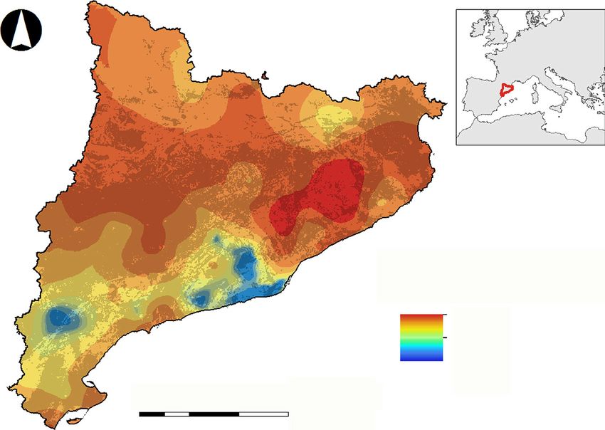
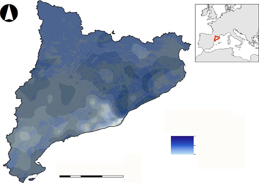
The maps of the smoothed relative risks of the study
SO2, sulphur dioxide; CO, carbon monoxide; O3, ozone; C6H6, benzene; H2S, hydrogen sulphide.
383
383
383
383
383
383
383
area and the a posteriori probabilities of such risks being
n
more than 1 are shown in Figures 1a and 2a and in Figures
1b and 2b respectively. These risks have been calculated
0.01 (0.003–0.06)
from a model than contains neither any explicative vari-
0.1 (0.04–0.1)
0.1 (0.03–0.2)
0.3 (0.2–0.6)
3.9 (1.8–7.5)
0.4 (0.2–0.9)
1.0 (0.5–1.6)
ables of interest nor any covariables but does contain ran-
dom effects and the expected cases in each census tract as
0.4 (0.3)
5.6 (6.0)
0.6 (0.5)
1.3 (1.1)
0.1 (0.1)
0.1 (0.4)
0.2 (0.3)
an offset. A certain pattern for the risk of incidence of ALS
is observed (Figs 1a, 2a) with clusters that coincide with
All
proximity to agricultural areas (Figs 1b, 2b). In Figure 2,
for example, 2 clusters with a high risk of occurrence of
766
766
766
766
766
766
766
ALS can be seen, one in the centre (direction north-
n
south), corresponding to the counties of Vallès Oriental
and Vallès Occidental, and another in the east (direction
south-east to north-east), corresponding to the country
of Maresme. There also seems to be a moderate-high-risk
cluster in the west, corresponding to the county of Baix
Llobregat (Fig. 2b).
Table 2 shows the results of the multivariate analysis.
Apart from the ORs and their credibility intervals at
Benzopirene, ng/m3, mean (SD)
95% (95% ICr), the probability of the parameter estima-
Cadmium, ng/m3, mean (SD)
tor (the log (OR) as an absolute value being more than
Arsenic, ng/m3, mean (SD)
Nickel, ng/m3, mean (SD)
C6H6, µg/m3, mean (SD)
Lead, ng/m3, mean (SD)
1 (Prob) is also shown (note that it is unilateral and so
H2S, µg/m3, mean (SD)
Table 1. (continued)
Median (Q1–Q3)
Median (Q1–Q3)
Median (Q1–Q3)
Median (Q1–Q3)
Median (Q1–Q3)
Median (Q1–Q3)
Median (Q1–Q3)
does not necessarily have to coincide with the ICr in all
the cases). Unlike the p value in a usual environment,
this probability allows us to make inferences about the
possible association. For the sake of simplicity, only the
Variables
results corresponding to the variables in which the Prob
of the associated coefficient (when it was included lin-
40 Neuroepidemiology 2018;51:33–49 Povedano/Saez/Martínez-Matos/Barceló
DOI: 10.1159/000489664Color version available online
Smoothed relative risks
High
Low
0 15 30 60 90
Kilometers
Fig. 1. a Map of the smoothed relative risks PRP (prob (RR >1))
over the study region (Catalonia). b Map High
over Catalonia of the posterior probability
that the smoothed relative risks were great- Low
er than unity (PRP). Model with heteroge-
neity and spatial adjustment only (besides 0 15 30 60 90
the expected cases in the census tract as an Kilometers
offset), without explanatory variables [1].
early in the model), or of at least one of the coefficients The same occurred, albeit less markedly, for patients
associated with its categories (when it was included cat- who lived between 100 and 199 m from an agricultural
egorically) being more than 0.80 are shown. An asso- zone (OR 1.559; 95% ICr 0.809–3.012; Prob 90.75%).
ciation is shown to exist between the occurrence of ALS Moreover, living between 25 and 100 m from the near-
and the distance from the residence of the subject to the est road increased the risk of being affected by ALS
nearest agricultural area. Patients who lived less than compared with living more than 100 m from it (OR
100 m from an agricultural area were at greater risk of 1.364; 95% ICr 0.885–2.104; Prob 91.99%). An associa-
being affected by ALS than those who lived further tion was also found between some atmospheric con-
away (OR 5.483; 95% ICr 1.279–25.23, Prob 98.93%). taminants and the incidence of ALS. More specifically,
Long-Term Exposure to Environmental Neuroepidemiology 2018;51:33–49 41
Factors and the Occurrence of ALS DOI: 10.1159/000489664Color version available online
Smoothed relative risks
High
Low
0 5 10 20 30
Kilometers
PRP (prob (RR >1))
Fig. 2. a Map of the smoothed relative risks
over the Metropolitan Area of Barcelona. b High
Map over the Metropolitan Area of Barce-
lona of the posterior probability that the Low
smoothed relative risks were greater than
unity (PRP). Model with heterogeneity and
spatial adjustment only (besides the ex- 0 5 10 20 30
pected cases in the census tract as an offset), Kilometers
without explanatory variables [1].
a non-linear and statistically significant relation was 92.62%) and between benzopireno and ALS, although
found to exist in the case of NO2, which presented an in this case, the association was not statistically signifi-
increasing gradient for the OR (OR quartile 2 1.872; cant (OR 1.122; 95% ICr 0.359–4.140; Prob 85.39%).
95% ICr 1.487–2.023; Prob 99.73%; OR quartile 3 2.047; Last, exposure to ozone was found to have a protector
95% ICr 1.698–2.898; Prob 99.73%; OR quartile 4 2.703; effect on the incidence of ALS (OR 0.973; 95% ICr
95% ICr 1.265–3.255; Prob 99.84%), and in the case of 0.949–1.061; Prob 92.67%).
NO, although in this case only the fourth quartile was Finally, with the idea of observing a possible synergy
statistically significant (and only at 90%; OR quartile 4 between living near agricultural areas (less than 100 m)
1.321; 95% ICr 0.530–3.340; Prob 92.71%). A linear as- and other environmental variables, the interactions be-
sociation was found between cadmium and the occur- tween living less than 100 m from agricultural areas and
rence of ALS (OR 1.332; 95% ICr 0.729–13.71; Prob living near traffic routes were introduced into the model,
42 Neuroepidemiology 2018;51:33–49 Povedano/Saez/Martínez-Matos/Barceló
DOI: 10.1159/000489664Table 2. Association between environmental variables and occurrence of ALS, Catalonia 2011–2016
Variables OR (95% credibility interval) Prob ([log(OR)]) >0
Distance agricultural areas (>300 m), m
100 m), m
200 m), m
300 m), m
150 m) 0.502 (0236–1.044) 0.8674
Distance green areas (quintile 1)
Quintile 2 0.910 (0.481–1.715) 0.6145
Quintile 3 1.283 (0.686–2.403) 0.7814
Quintile 4 0.834 (0.437–1.593) 0.7058
Quintile 5 1.381 (0.662–2.910) 0.8034
Daytime environmental noise (quintile 1)
Quintile 2 4.531 (0.290–106.8) 0.8447
Quintile 3 0.528 (0.009–36.06) 0.6255
Quintile 4 0.085 (0.001–6.692) 0.8693
Quintile 5 0.386 (0.004–37.10) 0.6635
Evening-time environmental noise (quintile 1)
Quintile 2 0.443 (0.018–7.500) 0.6931
Quintile 3 4.956 (0.055–380.1) 0.7632
Quintile 4 29.14 (0.294–2,587) 0.8261
Quintile 5 13.12 (0.104–1,499) 0.8538
Night-time environmental noise (quintile 1)
Quintile 2 1.437 (0.438–4.539) 0.7305
Quintile 3 0.886 (0.199–3.865) 0.5631
Quintile 4 0.817 (0.149–4.381) 0.5930
Quintile 5 0.439 (0.065–2.926) 0.8031
NO2 (quartile 1)
Quartile 2 1.872 (1.487–2.023) 0.9973
Quartile 3 2.047 (1.698–2.898) 0.9973
Quartile 4 2.703 (1.265–3.255) 0.9984
NO (quartile 1)
Quartile 2 0.515 (0.140–1.958) 0.7216
Quartile 3 0.329 (0.074–1.482) 0.8394
Quartile 4 1.321 (0.530–3.340) 0.9271
Benzopirene 1.122 (0.359–4.140) 0.8539
Cadmium 1.332 (0.729–13.71) 0.9262
Ozone 0.973 (0.949–1.061) 0.9267
Adjusted by sex, age, year of diagnosis, family history of disease, indicator of family in the database, contex-
tual deprivation index.
Prob (abs [log(OR)] >0) higher than 0.95. Prob (abs [log(OR)] >0) higher than 0.90.
Long-Term Exposure to Environmental Neuroepidemiology 2018;51:33–49 43
Factors and the Occurrence of ALS DOI: 10.1159/000489664as well as living in areas with high levels of atmospheric them included in a single municipality) in all Italian
contamination. Only the interactions with the fourth municipalities in the period 1980–2001 and suggest, in
quartiles of NO2 (OR 1.094, Prob 98.62%) and NO (OR addition to genetics, that agricultural chemicals and
1.124, Prob 98.70%) were statistically significant. Fur- lead could be involved. However, very recently, Tes-
thermore, the fourth quartile of benzopirene and liv- auro et al. [14], investigated an ALS cluster reported in
ing less than 100 m from a dual carriageway or a motor- the Briga area (in the province of Novara, northern It-
way, even when they were risk factors and where the aly), known for its high level of heavy metal contamina-
probability of the odds ratio being more than the unit was tion, which has had a serious impact on soil, surface
over 85% in both cases, were not statistically significant. water and groundwater, but they could not confirm an
It must be pointed out that unlike the main effect, the in- excess of ALS incidence.
teraction between living less than 100 m from agricul- Our results could be in line with the findings of those
tural areas and in an area with high levels of ozone (lo- studies, particularly with those that attribute in some way
cated in the fourth quartile) was a risk factor (OR 2.484, to the exposure to agricultural chemicals [80, 81]. In this
Prob 88, 22%). sense, all the clusters we identified correspond to areas of
intensive agriculture. In our case, the high-risk clusters,
besides corresponding to agricultural areas, also corre-
Discussion spond to significant road infrastructures that carry a high
density of traffic. In fact, our hypothesis could be cor-
We found a certain geographical pattern for the risk roborated by the results of the interactions of those living
of ALS occurrence. In addition, 3 clusters can be ob- less than 100 m from an agricultural area and high levels
served, 2 of them with a high risk of occurrence of ALS – of nitrogen oxides (significant at 95%), benzopyrene and
one in the centre of the study region (north-south direc- ozone (significant at 85%) as well as for those living less
tion) and another in the east (direction southwest-north- than 100 m away from dual carriageways and motorways
east), and the third one with a moderate-high risk in the (significant at 85%).
west. The results of the multivariate model suggest that
As mentioned above, there is enough evidence, in- these clusters could be related to some of the environ-
cluding some systematic reviews [18, 20, 22–25], of the mental variables. Specifically, living near an agricultural
existence of spatial clusters of ALS. However, only in area increased the risk of ALS occurrence (especially for
some of them have environmental factors been suggest- less than 100 m and in a smaller magnitude between 100
ed as a possible explanation for their occurrence [14, 48, and 199 m). In addition, air pollution resulting from
76–82]. This is particularly notable for exposure to met- traffic could also be related to the occurrence of ALS.
als [48, 77, 80, 81] and to agricultural chemicals [78– Thus, besides living between 25 and 100 m from a resi-
81], although exposure to industrial toxins [77] and to dential street, high NO2 and NO concentrations in the
paper paste and water treatment plants [82] also ap- air where the subject resides, indicated a greater risk of
pears. As early as 1977, Kilness and Hichberg [76] at- occurrence of ALS. We also found a statistically signifi-
tributed selenium exposure over a period of 10 years to cant association between exposure to ozone and the oc-
the small cluster (4 ALS cases that lived within 15 km currence of ALS. In addition, we found a linear associa-
of each other) that they identified in west-central South tion between benzopyrene levels in the air and the oc-
Dakota, USA. Almost 30 years ago, Sienko et al. [48] currence of ALS (albeit not statistically significant).
detected a cluster in a small fishing village next to Lake Benzopyrene belongs to the chemical class of polycyclic
Michigan, USA, which is probably associated with a aromatic hydrocarbons, ubiquitous compounds of
high intake of mercury. In addition to genetics, among which one of the sources is motor vehicle exhaust fumes.
the factors to which Sabel et al. [80] attribute the exis- The statistically significant associations found for cad-
tence of 2 significant clusters in south-eastern Finland mium and, to a lesser extent, benzopyrene (another
(one at the time of death and other at the time of birth, source for this is the chemical industry), could suggest
of those who died between 1985 and 1995) and another some relationship between emissions from industrial
in south-central Finland (at the time of death) is the activities and the occurrence of ALS. In fact, cadmium
exposure to heavy metals and agricultural chemicals. emissions come mainly from industrial processes using
Similarly, Uccelli et al. [81] identified 16 clusters with combustion chiefly derived from inorganic chemical
significant high relative risk of ALS mortality (12 of compounds [83].
44 Neuroepidemiology 2018;51:33–49 Povedano/Saez/Martínez-Matos/Barceló
DOI: 10.1159/000489664We considered the distance (from the subject’s home) higher risk of occurrence of ALS, are those with a lower to the agricultural area as a proxy for pesticide exposure. concentration of ozone. The results from the interac- In fact, and as can be seen, we followed a strategy similar tions of living less than 100 m from an agricultural area to that of the studies suggesting agricultural chemicals as and high levels of ozone (significant at 85%) could be an explanation for the high-risk clusters of ALS occur- indicative of this fact. High levels of ozone would occur rence [80, 81], as well as the strategy used by Das et al. in suburban or rural areas and, therefore, close to the [84], in a case-control study carried out from 2008 to agrarian zones. In those areas, we find that interaction 2011 in India. Here, they found (in addition to electrical is a risk factor. However, in our case, most ALS cases injury – OR 1.62-; and smoking – OR 1.88-) that not only were collected in urban areas. For this reason, the inter- exposure to pesticides (OR 1.61) but also living in a rural action was significant only at 85%. habitat (OR 1.99) were the associated factors in the occur- In line with the systematic review by Tzivian et al. [55], rence of ALS. They argue that rural people are exposed to we found that, once air pollutants have been controlled, insecticides and pesticides during their occupational none of the indicators of environmental noise is related work in agriculture and also when drinking water which, to the occurrence of ALS either directly (levels of the con- in their study region (east of India), may sometimes be taminant) or indirectly (through the proxies of distance contaminated with insecticides and pesticides [84]. As- to roads). However, more studies are needed to deter- suming that the distance to agricultural areas was a good mine if the role of environmental noise can be indepen- proxy for exposure to pesticides, our results would be in dent to that of air pollutants. line with those where associations between exposure to Our study might have some limitations. First, although pesticides and the occurrence of ALS have been made we included an offset in the model to control for these ef- [27–36, 38]. fects, the original cohort consisted of a non-random sam- Although there are only a few studies that relate ex- ple. However, it would seem that the sample we used was, posure to air pollutants as a result of traffic and the oc- in fact, quite representative. First, we estimated a preva- currence of ALS [32, 53, 54], our results are similar. lence of ALS at 5.09 per 100,000 inhabitants, (i.e., within Seelen et al. [54] in particular, find that, as in our case, the range indicated in the literature [5–5.4] [9, 14]), and once adjusted for possible confounders, the risk of ALS a crude incidence at 1.12 per 100,000 person/years (95% is significantly higher for subjects with high levels of CI 0.85–1.48), an interval containing the incidence esti- exposure to NO2. Unlike them, however, we did not mated by Pradas et al. [12], for Catalonia (1.4 per 100,000 find an association between PM2.5 absorbance concen- inhabitants). Second, the male/female ratio in the inci- trations and the occurrence of ALS. As in Vinceti et al. dence in our sample was only slightly less than that re- [39], neither did we find a significant association with ported in the literature [15, 10, 12] (1.25 vs. 1.3–1.5 ALS and the polycyclic aromatic hydrocarbon benzopy- respectively). The mean age of the cases was 63.22 years rene. and the median age was 65 years. These figures corre- We do not have an explanation for the protective ef- sponded to the mean age at onset, which ranges from 58 fect found for ozone exposure. One possibility is that to 63 years for the sporadic form and 40 to 60 years for antagonistic interactions occur between ozone and ni- the familial form [9]. trogen dioxide [85]. In addition, ozone levels tend to be Third, we did not know the family history of the con- lower in urban areas than in suburban and rural areas. trols and, therefore, we did not know if they had a family This is because it is a secondary pollutant that does not history of ALS in a first or second-degree blood relative. appear immediately. There is a gap between the emis- However, much of this limitation is avoided by the strat- sion of precursors and its formation. Furthermore, egy we followed when choosing the controls. The controls winds can carry polluted air masses out of the cities and were subjects, alive and free of ALS and other neurode- direct them towards the peripheral or rural areas. On the generative diseases at each failure time and, therefore, other hand, the highest concentrations of ozone do not they were still at risk at the time of the failure of the case, occur near the emission source but rather a certain dis- no matter their family history. tance away from it because the ozone that forms in the Fourth, we used proxies to approximate exposure to proximities of the focus reacts with the existing nitrogen environmental variables (especially distances). We were monoxide and destroys itself in the proximity of the not able to determine to which particular variable or to source [86]. Therefore, it is likely that the areas with the what amount of environmental variable the subject was most air pollution as a result of traffic, and those with a exposed to. We believe, however, that we controlled part Long-Term Exposure to Environmental Neuroepidemiology 2018;51:33–49 45 Factors and the Occurrence of ALS DOI: 10.1159/000489664
You can also read