Impacts of Extreme Climate Events on Technical Efficiency in Vietnamese Agriculture
←
→
Page content transcription
If your browser does not render page correctly, please read the page content below
# 2019-100

        Impacts of Extreme Climate Events on
    Technical Efficiency in Vietnamese Agriculture

         Yoro DIALLO*, Sébastien MARCHAND †, Etienne ESPAGNE ‡

                                           March 2019

Please cite this paper as:      DIALLO, Y., S. MARCHAND and E. ESPAGNE (2019), “Impacts of Extreme
                                Climate Events on Technical Efficiency in Vietnamese Agriculture”, AFD
                                Research Papers Series, No. 2019-100, March.

Contact at AFD:                 Etienne ESPAGNE (espagnee@afd.fr)

*    Université de Clermont Auvergne, CNRS, CERDI.
†    Université de Clermont Auvergne, CNRS, CERDI.
‡    AFD, CERDI.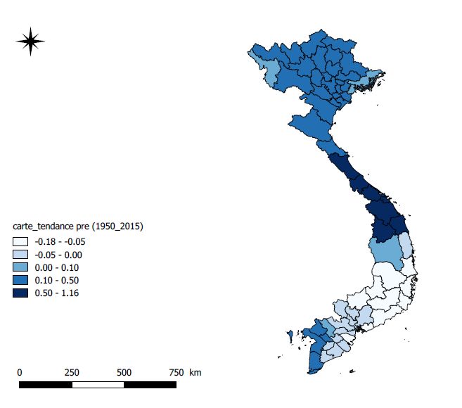
Agence Française de Développement / French Development Agency
Papiers de Recherche de l’AFD
Les Papiers de Recherche de l’AFD ont pour but de diffuser rapidement les résultats de travaux en
cours. Ils s’adressent principalement aux chercheurs, aux étudiants et au monde académique. Ils
couvrent l’ensemble des sujets de travail de l’AFD : analyse économique, théorie économique, analyse
des politiques publiques, sciences de l’ingénieur, sociologie, géographie et anthropologie. Une
publication dans les Papiers de Recherche de l’AFD n’en exclut aucune autre.
L’Agence Française de Développement (AFD), institution financière publique qui met en œuvre la
politique définie par le gouvernement français, agit pour combattre la pauvreté et favoriser le
développement durable. Présente sur quatre continents à travers un réseau de 72 bureaux, l’AFD
finance et accompagne des projets qui améliorent les conditions de vie des populations, soutiennent la
croissance économique et protègent la planète. En 2014, l’AFD a consacré 8,1 milliards d’euros au
financement de projets dans les pays en développement et en faveur des Outre-mer.
Les opinions exprimées dans ce papier sont celles de son (ses) auteur(s) et ne reflètent pas
nécessairement celles de l’AFD. Ce document est publié sous l’entière responsabilité de son (ses)
auteur(s).
Les Papiers de Recherche sont téléchargeables sur : https://www.afd.fr/fr/ressources
AFD Research Papers
AFD Research Papers are intended to rapidly disseminate findings of ongoing work and mainly target
researchers, students and the wider academic community. They cover the full range of AFD work,
including: economic analysis, economic theory, policy analysis, engineering sciences, sociology,
geography and anthropology. AFD Research Papers and other publications are not mutually exclusive.
Agence Française de Développement (AFD), a public financial institution that implements the policy
defined by the French Government, works to combat poverty and promote sustainable development.
AFD operates on four continents via a network of 72 offices and finances and supports projects that
improve living conditions for populations, boost economic growth and protect the planet. In 2014, AFD
earmarked EUR 8.1bn to finance projects in developing countries and for overseas France.
The opinions expressed in this paper are those of the author(s) and do not necessarily reflect the
position of AFD. It is therefore published under the sole responsibility of its author(s).
AFD Research Papers can be downloaded from: https://www.afd.fr/en/ressources
AFD, 5 rue Roland Barthes
75598 Paris Cedex 12, France
ResearchPapers@afd.fr
ISSN 2492 - 2846Impacts of Extreme Climate Events on Technical Efficiency in Vietnamese Agriculture Yoro Diallo, Université de Clermont Auvergne, CNRS, CERDI Sébastien Marchand, Université de Clermont Auvergne, CNRS, CERDI Etienne Espagne, AFD, CERDI Abstract The aim of this study is to examine farm household-level impacts of weather extreme events on Vietnamese rice technical efficiency. Vietnam is considered among the most vulnerable countries to climate change, and the Vietnamese economy is highly dependent on rice production that is strongly affected by climate change. A stochastic frontier analysis is applied with census panel data and weather data from 2010 to 2014 to estimate these impacts while controlling for both adaptation strategy and household characteristics. Also, this study combines these estimated marginal effects with future climate scenarios (Representative Concentration Pathways 4.5 and 8.5) to project the potential impact of hot temperatures in 2050 on rice technical efficiency. We find that weather shocks measured by the occurrence of floods, typhoons and droughts negatively affect technical efficiency. Also, additional days with a temperature above 31°C dampen technical efficiency and the negative effect is increasing with temperature. For instance, a one day increase in the bin [33°C-34°C] ([35°C and more[) lessen technical efficiency between 6.84 (2.82) and 8.05 (3.42) percentage points during the dry (wet) season. Keywords: Weather shocks, Technical efficiency, Rice farming, Vietnam JEL Classification: D24, O12, Q12, Q54 Original version: English Accepted: March 2019
Impacts of Extreme Climate Events on Technical
            Efficiency in Vietnamese Agriculture
             Yoro Diallo*, Sébastien Marchand†and Etienne Espagne‡

                                         March 12, 2019

                                              Abstract

          The aim of this study is to examine farm household-level impacts of weather ex-
       treme events on Vietnamese rice technical efficiency. Vietnam is considered among
       the most vulnerable countries to climate change, and the Vietnamese economy is
       highly dependent on rice production that is strongly affected by climate change.
       A stochastic frontier analysis is applied with census panel data and weather data
       from 2010 to 2014 to estimate these impacts while controlling for both adaptation
       strategy and household characteristics. Also, this study combines these estimated
       marginal effects with future climate scenarios (Representative Concentration Path-
       ways 4.5 and 8.5) to project the potential impact of hot temperatures in 2050 on
       rice technical efficiency. We find that weather shocks measured by the occurrence of
       floods, typhoons and droughts negatively affect technical efficiency. Also, additional
       days with a temperature above 31°C dampen technical efficiency and the negative
       effect is increasing with temperature. For instance, a one day increase in the bin
       [33°C-34°C] ([35°C and more[) lessen technical efficiency between 6.84 (2.82) and
       8.05 (3.42) percentage points during the dry (wet) season.
          Keywords: Weather shocks, Technical efficiency, Rice farming, Vietnam
          JEL Classification: D24, O12, Q12, Q54.

   *
      Corresponding author: yoro.diallo@uca.fr; Université Clermont Auvergne, CNRS, CERDI
   †
      sebastien.marchand@uca.fr; Université Clermont Auvergne, CNRS, CERDI
    ‡
      espagnee@afd.fr; AFD, CERDI. Acknowledgements: This work is part of the GEMMES Vietnam
project, launched by the Agence Française de Développement in order to study the socio-economic impacts
of climate change and adaptation strategies to climate change in Vietnam. It belongs to the ECO package.
We are thankful to Nicolas De Laubier Longuet Marx, Olivier Santoni, Ngo Duc Thanh and the GEMMES
team for helpful comments.

                                                   1
1 Introduction
Given the increasing awareness about climate change and the growing concern about
its downside consequences, the question of a quantitative assessment of the economic
consequences of climate change is of great importance. This issue is particularly topical
in countries heavily exposed to the risks of weather variability and climate change like
Vietnam which is among the countries most vulnerable to climate change according to the
Climate Change Knowledge Portal (CCKP) of the World Bank1 . Since the country lies
in the tropical cyclone belt, it is heavily exposed to climatic-related risks like droughts,
floods, tropical storms (typhoons), rising sea level and saltwater intrusion (Bank, 2010).
This vulnerability is also increased by the topography of the country. Vietnam is a
long narrow country consisting of an extensive coastline of more than 3,000 km long
subjected to accelerated erosion and rising sea level. It contains two major river deltas
(the Mekong delta in the South and the Red River delta in the North) highly exposed to
floods and rising sea level (Dasgupta et al., 2007), which concentrate a high proportion
of the country’s population and economic assets such as rice farming, and mountainous
areas on its eastern and northeastern borders.
In Vietnam, rice farming has played a central role in economic development since
1980 and the beginning of market and land reforms2 . Paddy rice is by far the main crop
produced in Vietnam and employs two thirds of total rural labor force. However, it is
also one of the most climate-change affected sectors due to its direct exposure to, and
dependence on, weather and other natural conditions (Bank, 2010). The ongoing climate
change and its related effects have and will have significant impacts on rice production
and farmer livelihoods. From census data between 2010 and 2014, and weather data
on temperature and precipitation, this study examines farm household-level impacts of
weather shocks, defined as extreme events such as extreme temperatures, floods, droughts
and typhoons, on agricultural productivity in the Vietnamese rice farming3 .
This study contributes to the growing literature that uses farm-level panel data (here
the Vietnam Household Living Standard Survey (VHLSS)) coupled with finely-scaled cli-
mate data to estimate the weather change impacts, here on Vietnamese rice farming (Yu
et al., 2010; Trinh, 2017). The use of a panel structure allows to control for time-invariant
omitted variables correlated with weather extreme events that may confound the climatic
1
Source: the CCKP website.
2
These last years, while the contribution of Vietnamese farming to national GDP has become less
important (from about 40% in 1990 to about 18% in 2016), rural areas still generate employment and
income for a significant part of the population (Bank, 2010). In 2016, 66% of the population live in rural
areas where 43% of the country’s active workforce is employed.
3
This study investigates weather impacts rather than climate impacts (Auffhammer et al., 2013).
More precisely, the former is defined as the conditions of the atmosphere over a short time horizon while
the latter is the variability of the conditions of the atmosphere over a relatively long period. Thus, the
interpretation of the coefficients associated with climatic variables have to be interpreted as weather
shocks in the short run and climate change in the long run.
2effect in pure cross-sectional studies (Blanc and Schlenker, 2017). Also, we study two
weather effects on rice farming from a Stochastic Frontier Analysis (SFA). We first esti-
mate the effect of weather trend, defined as the mean daily temperature and the mean
daily precipitation, on rice farming output. Then, we assess the effect of weather extreme
events, measured by the occurrence of floods, typhoons, droughts and extreme tempera-
tures, on rice farming productivity defined as technical efficiency4 . As a result, we find
that weather shocks measured by the occurrence of floods, typhoons and droughts nega-
tively affect technical efficiency. Also, daily temperatures above 31°C dampen technical
efficiency in the dry season, an effect which is increasing with temperature. For instance,
a one day increase in the bin [33°C-34°C] lowers technical efficiency between 6.84 and 8.05
percentage points. Simulation results show dramatic drops in technical efficiency after
2040. In the case of the RCP8.5 scenario, technical efficiency collapses from 40%, while
it stabilizes in the RCP4.5 scenario around 10% below the reference period5 .
The remaining of the paper is organized as follows. Section 2 presents the literature
related to the climate-agriculture nexus. Section 3 details the rice sector and climate
conditions in Vietnam. Sections 4, 5 and 6 present respectively the empirical methodology,
data and descriptive statistics, and econometric results. Section 7 gives the results from
simulations and Section 8 concludes.
2 Literature reviews
This section reviews the theoretical and empirical studies that estimate the economic
impact of climate change on agriculture. The literature can be divided between the long-
run climate effect approach using the Ricardian hedonic model with cross-sectional data
(see Mendelsohn and Massetti (2017) for a discussion of main advantages and weaknesses
of this approach), and the weather-shock approach using Ricardian hedonic model with
panel data (see Blanc and Schlenker (2017) for a discussion of main advantages and
weaknesses of this approach).
The first approach consists in examining how the long-run climate (the distribution of
weather over 30 years) affects the net revenue or land value of farms across space using
the Ricardian method (also called the hedonic approach). The principle of this method is
to estimate the impact of climate on agricultural productivity by regressing net revenue
or farmland value (use as a proxy for the expected present value of future net revenue)
on climate in different spatial areas. The model assumes that competitive farmers are
profit-maximizing agents. Farmers choose an optimal combination of inputs and output
4
To our knowledge, only Key and Sneeringer (2014) use a SFA methodology to study heat stress on
technical efficiency on dairy production in United States.
5
We only used one CORDEX-SEA model for climate projections in this version of the paper, which
limits the level of confidence we can have for these projections. We will use all the existing simulations
as soon as they are available, so that we can discuss the uncertainty issue about future climates.
3to maximize net agricultural income, subject to the exogenous variable such as climatic
conditions that are beyond the farmer’s control. Put differently, if climate is different, the
farmer has to adapt his production and choose a different output (crop switching) and
different inputs (new pesticides for instance). This is probably the main advantage of the
Ricardian approach that allows to capture long-run adaptation to climate. So the goal is
to regress net revenue on different arrays of climates to estimate the impact of climate.
According to Mendelsohn and Massetti (2017), this approach has been used in 41 studies
over 46 countries. The first attempt is Mendelsohn et al. (1994) who estimate the impact
of temperatures on land prices in 3,000 counties in the United States. They found from
simulation based to the econometrically estimated impacts of temperature that global
warming may have economic benefits for the U.S. agriculture.
This initial approach has been then improved in different ways to take into account
many empirical issues. One of them concerns the measure of climate. Most studies used
seasonal climate variables but the type of variable changes from one study to another.
Some studies include mean seasonal temperature and rainfall (Mendelsohn et al., 1994;
Schlenker et al., 2005) while other use the degree days over the growing season that are
the sum of temperatures above a floor (Schlenker et al., 2006; Deschênes and Greenstone,
2007)6 .
Another important empirical issue is related to the cross-sectional nature of the method.
In fact, many existing studies estimate a Ricardian model using data for a single year or
two. However, a main disadvantage of cross-sectional data is potential omitted variables
that might bias the results since average climate over a long period is not random across
space. For instance, Dell et al. (2009) find that poorer countries tend to be hotter. But
this relationship can be considered as spurious correlation if there are some omitted vari-
ables correlated with climate that can explain income (institutions for instance). The
model has to control for these potential omitted variables. Two solutions have been de-
veloped in the literature to avoid omitted variable bias. The first solution is to account for
all factors that are both correlated with climate and the impacted farmland values. One
first example is irrigation that is correlated with temperature. For instance, Schlenker
et al. (2005) show that access to subsidized irrigation water is both capitalized into farm-
land values and correlated with hotter temperatures. This means that the impacts of
irrigation has to be control while estimating the impact of temperature on land value.
If not, the regression estimates not only the direct effect of temperature, but also the
beneficial effect of access to irrigation water (which is positively correlated with higher
temperatures). To resolve this issue, Schlenker et al. (2005) separate irrigated and rain-
fed farms and estimate models for each sample. Another solution is the one implemented
6
See Massetti et al. (2016) for a discussion of these two approaches and the pitfalls of the degree days
approach with the Ricardian method. Note that this issue concerns also the weather approach discussed
infra.
4by Kurukulasuriya et al. (2011). The authors first estimate the probability of making the
irrigation choice and then estimate the conditional Ricardian model given the choice of
making irrigation. However, this solution can never completely eliminate the possibility
of omitted variables. In fact, there might always be an additional control variable (e.g.
soil quality) that is correlated with climate (e.g. temperature) but unfortunately not
correlated with the other control variables (e.g. irrigation) included in the specification.
The second solution may address this concern and consists in using panel data into
the Ricardian model (i.e., estimate long-run climate impact) (Deschênes and Greenstone,
2007). Panel data allow for the use of fixed effects, which control for any time-invariant
confounding variation. However, in a model with fixed effects, it is impossible to estimate
the effect of the long-run climate averages because climate has no temporal variation.
However, while Deschênes and Greenstone (2007) show that the Ricardian results are
not robust when estimated as a series of repeated cross sections, Schlenker et al. (2006);
Massetti and Mendelsohn (2011) provide evidences that the Ricardian model is stable
when estimated with panel methods. Massetti and Mendelsohn (2011) for instance provide
two robust methods to estimate Ricardian functions with panel data: (1) a two-stage
model based on Hsiao (2014) where agricultural outcome is regressed on time varying
variables using the covariance method with fixed effects and then, in the second stage,
the time-mean residuals from stage 1 are regressed on non-varying time variables such as
climate variables (also used by Trinh (2017)); (2) a single stage “pooled” panel model.
While the Hsiao model is less vulnerable to the omitted variable bias than the pooled
panel model, it is less efficient than the pooled panel model estimated in one step. The
main result of Massetti and Mendelsohn (2011) is that the overall effect of climate change
is likely to be beneficial to U.S. farms over the next century.
The second main approach is the weather-shock approach using Ricardian hedonic
model with panel data (Schlenker and Roberts, 2009; Schlenker et al., 2013; Deryugina
and Hsiang, 2017). The starting point of this approach is to take advantage of fine-scaled
weather data in both time and space to detect for instance nonlinearity through the large
degree of freedoms that give panel data. For instance, Schlenker and Roberts (2009) find
a non-linear relationship between temperature and U.S. crop production. Beyond the
respective thresholds of 29°, 30° and 32°, the temperature generates major damage on
wheat, soybean and cotton yields respectively. Also, this approach allows to avoid the
omitted variable bias by controlling for fixed effects. Another advantage of this approach
is to account for short-term adaptation. Although panel analysis allows for spatial and
temporal heterogeneity, it is not free of limits (Blanc and Schlenker, 2017). One of them
is the consideration of spatial autocorrelation in crop yields and climatic variables which
is necessary in order to limit the estimation bias. Chen et al. (2016) take this criticism
into account in their analysis of the link between climate change and agricultural sector
in China. They find that Chinese agricultural productivity is affected by the trend in
5climate and the existence of a non-linear and U-inversed shape between crop yields and
climate variability.
Our study uses the weather-shock approach with panel data. However, instead of
using a Ricardian hedonic model, we follow Key and Sneeringer (2014) and estimate the
relationship between weather and rice farming productivity defined as technical efficiency
using a stochastic production frontier model.
3 Rice production and climate condition in Vietnam
3.1 Rice production in Vietnam
Since the beginning of the Vietnam’s Đổi Mới (renovation) process launched in 1986, Viet-
nam has witnessed unprecedented transitions from planned and collectivized agriculture
to market and household-based farming.
The market reform periods of Vietnamese rice farming began with the output contracts
period (1981–87) which launched the move to de-collectivize agriculture (Kompas et al.,
2002, 2012). It was the first attempt towards private property rights. Farmers were
allowed to organize production activities privately but the most part of rice production
had still to be sold in state markets at low state prices. However, private domestic
markets emerged for some portion of output sold (approximately 20%). This period was
thus characterized by a “dual price” system (a low state price and a competitive market
price) with strict state controls.
From 1988 on, the period of trade and land liberalization began with the aim to
establish effective private property rights over both land (initially 10–15 year leases) and
capital equipment while restrictions on farm size and prohibitions against the removal of
land from rice production were maintained. In 1990 the central government abolished the
dual price system and rice was authorized to be sold on competitive domestic markets.
However, while those reforms were intended to incite farmers to invest, in practice, farmers
were reluctant to undertake long-term investments because the land-use rights were not
seen as secure as they were not tradable. Consequently, the government passed a new
Land Law in 1993. This law extended the lease period to twenty years for land used to
produce rice (increased to 30 years in 1998 revisions) and allowed farmers to transfer,
trade, rent, mortgage and inherit their land-use rights (Scott, 2008). Also, from 1993,
farmers could now sell rice freely in international markets.
From the mi-1990s, land and market reforms implemented from 1981 allowed the
decentralization of production decisions at the farmer’s level and guaranteed that all farm
income (after tax) was retained by the farmer. Individual efforts were rewarded in order
to push farmers to invest and produce more. More recently, beyond these market and
land reforms, government implemented a rice policy helping to increase yield through the
6development of rice varieties, large investment in irrigation (roughly 85% of rice area are
applied with active irrigation drainage system), the support in case of emergency cases,
the ease of credit access, input support (reducing valued-added tax for key inputs as
fertilizers), etc.
As a consequence, Vietnam has become the fifth rice producer in the world with a
total production of 42.76 millions of tons per year and a yield of 5.55 tons per hectare in
2017, a lot more than annual 12.4 millions of tons produced and the yield of 2.19 tons per
hectare in 1980, and a leading world exporter (about 7 millions tons)7 .
Regarding the geographical distribution of rice production, rice area covers roughly
7,8 millions hectares (23% of total land area and 82% of arable land) owned by 9 millions
of households (accounting for more than 70% of rural households) so that the average
farm size is below one hectare. Rice area is located mostly in the Mekong River Delta
(about 55% of total rice production (23 millions of tons produced in 2017) and 90% of
rice exports) followed by the Red River Delta in the northeast (about 15% of total rice
production) and the north-central coast8 .
Despite the increase of the yield in rice production these last decades, some important
pitfalls remain. For instance, rural inputs and land markets or access to agricultural ex-
tension services and farm credit remain still far less developed in some provinces, trapping
farmers into poverty (Kompas et al., 2012). Also, the expansion of rice production for the
last thirty years was reached by focusing on quantity increases. The abuse of chemical
inputs (Berg and Tam, 2012) produce important environmental damages in terms of soil
fertility or depletion of fishery resources for instance. Besides, past international successes
of Vietnamese rice production was based mainly on high production of low quality rice
sold at very low price on international markets, a strategy that the recent increase in in-
put prices (fertilizer, fuel, and labor) could well jeopardize (Demont and Rutsaert, 2017).
Vietnamese rice farming now has to deal with significant issues both at national and inter-
national levels. At the national level, Vietnamese farming has to deal both with poverty
alleviation of rice households (by encouraging crop diversification on rice), food security
(feeding both Vietnamese with good quality rice products) and environmental preserva-
tion (by promotion organic rice farming, soil preservation, etc.) (Tran and Nguyen, 2015).
These national challenges have also implications at the international level. The compet-
itiveness of Vietnamese farming depends on the performance of farmers and companies
to deliver rice products with reliability regarding the quality (i.e. switching to high value
rice to follow change in world demand), safety and sustainability of the products supplied
(Demont and Rutsaert, 2017). Beyond these national and international issues, the ongo-
ing climate change is also an imperious issue that Vietnamese have to face in order to
preserve their rice production and the livelihood of millions of farmers.
7
Data come from FAOSTAT.
8
Data come from GSO, the general statistics office of Vietnam.
73.2 Climate condition
Seasonal variability of temperature and precipitation
Due to the diversity in topography, it is likely that the impacts of climate change will be
different depending both on the place and the months of the year. The curves in figure 1
transcribe the seasonal variations of the temperatures and precipitations according to the
months of the year. High temperatures are observed from May to October (the average
is 27.12°C) and lower temperatures from November to April (the average temperature
is 22.73°C). In addition, a greater instability of temperatures appears in the middle of
the year (an average amplitude of 2°C). Similarly precipitations are higher during the
period from May to October (an average rainfall of 238.20 mm) and relatively low from
November to April (an average rainfall of 68.93 mm). These observations allow us to
distinguish two major climatic seasons in Vietnam: a dry season (November to April)
and a wet season (May to October).
As in Hsiang (2010) and Trinh (2017), we use these seasonal temperature and precip-
itation variables to measure the impact of seasonal variability to test the dependence of
technical efficiency on the periodic occurrence of weather shocks. However, we are aware
that these time intervals can vary from one region to another throughout the country.
Figure 1: Seasonal variation of precipitation and temperature (1950-2015)
Seasonal variation of precipitation
500
400
(mean) preM
200 300
100
0
1 2 3 4 5 6 7 8 9 10 11 12
Month
Seasonal variation of temperature
30 25
(mean) tmpM
20 15
1 2 3 4 5 6 7 8 9 10 11 12
Month
Source: authors from CHIRPS and MODIS data
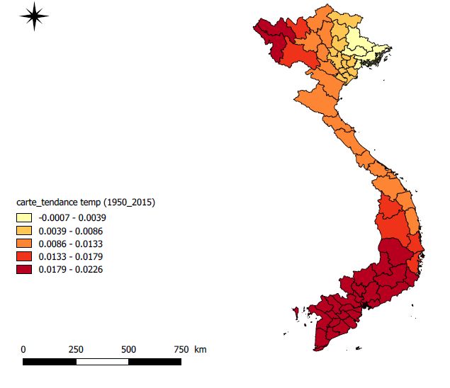
8Temperature and precipitation trends by Vietnamese regions (1950-2015)
Figures 2 and 3 represent the average trends in temperatures and precipitations over
the period 1950-2015 at sub-national levels. There is a strong spatial heterogeneity in
the variability of climatic conditions. The Mekong region in the south has experienced
a more pronounced global warming which is manifested by a mean annual temperature
trend increase of 0.02°C corresponding to an increase of 1.3°C over the period 1950-2015.
However, the temperature in the Red Delta region in the north-east remains pretty stable.
On the other hand, there is an average decrease in precipitations in the south, unlike
in the north and center where there has been a relative increase in monthly precipitations.
In addition, Figures A1 and A2 in Appendix respectively show the evolution of the level
of temperatures and precipitations according to the month of the year. In these figures,
we are able to perceive the occurrence of short-term climatic shocks by month and by
year.
9Figure 2: Average annual temperature trend increase over the period 1950-2015
Source: authors from MODIS data
10Figure 3: Average annual rainfall trend increase over the period 1950-2015
Source: authors from CHIRPS data
4 Empirical methodology
The link between agricultural productivity in rice farming and weather (trends and shocks)
is analyzed through a two-step approach. Agricultural productivity is first defined in terms
of technical efficiency calculated from a stochastic production frontier model in which
weather trend is also used to explain agricultural production. In the second step, the
estimated technical efficiency is explained by weather extreme events. Before presenting
the econometric model, we present the conceptual framework on which the econometric
analysis relies.
114.1 Conceptual framework
4.1.1 Definition of efficiency
Farrell (1957) defines agricultural productivity as productive efficiency which is the ability
of producers to efficiently use the available resources, called inputs hereafter, in order to
produce maximum output at the minimum cost. It differs from effectiveness that refers
to the degree of achievement of a desired goal. In addition, productive efficiency is the
combination of allocative efficiency (AE hereafter) and technical efficiency (TE hereafter).
AE is based on the optimal combination of inputs given their market prices, production
technology and the market prices of the output. It necessarily leads to the maximization
of profit or even the minimization of production costs. TE refers to the performance of
the producer to avoid waste of inputs to produce. This waste can be avoided in two
ways: either by reducing the quantity of inputs for the same level of production (the
input-oriented measure of TE), or by increasing the production for the same given level of
inputs (the output-oriented measure of TE). While AE is estimated from a profit function
or a cost function, TE is estimated from a production function. In this study, we work
on TE because we do not have price informations on inputs and output.
4.1.2 Estimation of technical efficiency
Technical efficiency is estimated under three auxiliary hypotheses regarding the choice
of the estimation method, the choice of the production function and the choice of the
functional form of TE over time.
Firstly, the estimation of TE relies on either the non-parametric method or the para-
metric method. The principle of the non-parametric method also called data envelopment
analysis (DEA) is to impose no restriction on the distribution of inefficiency, no behavioral
assumptions (goal of profit maximization) unlike the parametric method which is based
on the methods and techniques of econometric estimation. However, DEA imposes to con-
sider that all shocks to the value of output have to be considered as technical inefficiency
whereas some factors (ex. climatic conditions) are not related to producer behavior and
can directly affect the production frontier. This explains why parametric method is often
preferred in the literature, by using stochastic production functions called stochastic fron-
tier analysis (SFA)(Aigner et al., 1977; Meeusen and van Den Broeck, 1977). This method
allows the error term to have two components: a negative component that measures ineffi-
ciency and an idiosyncratic error that represents all other idiosyncratic shocks. However,
imposing on the inefficiency component to be negative requires strong assumptions about
its distribution law. The most used distributions are the half-sided normal law, the ex-
ponential law and the normal truncated law (Stevenson, 1980). The use of the half-sided
normal law and the exponential law assumes that the majority of the observation units
12are efficient relative to the truncated normal law9 .
Secondly, the form of the production function has to be chosen in a SFA technique. In
microeconomics, the production function expresses the relationship between outputs and
inputs. Its functional representation has to respect certain properties10 , taking into ac-
count the presence or not of economies scale and the nature of the substitutability between
inputs. The production function is often modelled using a Cobb-Douglas form (Cobb and
Douglas, 1928) or a transcendental logarithmic (“translog”) specification (Christensen
et al., 1971) in the literature. The Cobb-Douglas form is often preferred because it gives
convex and smoothed isoquantes. However, it is based on strong assumptions such as the
constancy of the elasticities and the hypothesis that all the elasticities of substitutions are
supposed to be equal to -1. More flexible forms of production such as the translog form
have emerged by not imposing restrictions on the production technology, especially with
regard to the substitution between inputs. In our analysis, we estimate the production
function by considering the translog form11 .
Thirdly, the estimation of TE in panel model implies to model the functional form
of TE over time. The first models are those of Pitt and Lee (1981) and Schmidt and
Sickles (1984) where inefficiency is supposed not to vary over time. This type of model
is comparable to a fixed effect in panel model. However, these models are based on very
strong assumptions. On the one hand, the model is valid under the assumption that
the inefficiency is uncorrelated with the inputs used to estimate the production function.
On the other hand, inefficiency has not to vary over time. Thus, other models emerged
to allow temporal variation of TE. However, the problem that has arisen concerns the
functional form of the temporal variation of inefficiency. Cornwell et al. (1990) proposes
the CSS model in which inefficiency varies with time according to a quadratic form.
While the temporal variation of TE is not necessarily quadratic, this hypothesis is very
restrictive. Battese and Coelli (1992) and Kumbhakar et al. (2000) develop a model in
which the temporal variation of the inefficiency term takes an exponential form. Lee and
Schmidt (1993) provide more flexibility in the form of temporal variation in inefficiency.
Their time-varying fixed-effects model does not impose restrictions on the functional form
of inefficiency. In other words, inefficiency is supposed to vary over time without imposing
a particular functional form on this variation. This model is particularly advantageous
for studies with a fairly large number of observation units and a relatively short time
dimension. This advantage also makes possible to circumvent the concern of incident
parameters (Chamberlain, 1979) potentially present with panel models12 .
9
The mode of the semi-normal law and the exponential law is equal to 0.
10
The production frontier requires monotonicity (first derivatives, i.e., elasticities between 0 and 1 with
respect to all inputs) and concavity (negative second derivatives). These assumptions should be checked
a posteriori by using the estimated parameters for each data point.
11
And the Wald test applied to interactive terms confirm the using of this model.
12
Other models such as Greene (2005) make it possible to dissociate the individual fixed or random
effect from TE. However, the large number of parameters to be estimated in these models is still subject
13In this study, we implement the stochastic frontier analysis by using both the Cobb-
Douglas and the translog production functions following the literature as well as the model
developed by Lee and Schmidt (1993) given that the time dimension of our base is quite
short (three years), while the number of farms is large (2,592 households).
4.2 Econometric strategy
We now apply the conceptual framework explained above to an econometric model in
agricultural production to firstly estimate TE and secondly to estimate the effects of
weather shocks on TE.
4.2.1 First step: Estimation of Technical Efficiency
Consider a farmer i at time t who uses x inputs (defined later) to produce rice defined by
y. The production function can be written as follows:
yi,t = f (xi,t ), (1)
where f is a function that defines the production technology. The rational producer
aims at maximizing his total production of rice while minimizing the total use of his
inputs. On the frontier, the farmer produces the maximum output for a given set of
inputs or uses the minimum set of inputs to produce a given level of output. Thus, the
definition of the production frontier and the estimation of technical efficiency depend on
the type of orientation: input-oriented or output-oriented. We use the output-oriented
measure of technical efficiency (more output with the same set of inputs) that gives the
technical efficiency of a farmer i as follows:
T Ei,t (x, y) = [maxϕ : ϕy ≤ f (xi,t )]−1 , (2)
where ϕ is the maximum output expansion with the set of inputs xi,t .
The output-oriented measure of technical efficiency defined by Eq. 2 is estimated
under three auxiliary hypotheses.
Firstly, Eq.1 is applied to an econometric model as follows:
yi,t = f (xi,t , β).e−Ui,t (3)
where yi is a scalar of output, xi is a vector of inputs used by farmers i=1,…,N, f (xi ; β)
is the production frontier and β is a vector of technology parameters to be estimated. Ui
are non-negative unobservables random variables associated with technical inefficiency
that follow an arbitrary half-sided distribution law.
to the incidental parameter concern.
14Secondly, we use a stochastic frontier analysis in which we assume that the difference
between the observed production and maximum production is not entirely attributed to
TE and can also be explained by idiosyncratic shocks such as weather. Eq.3 becomes:
yi,t = f (xi,t , β).e−Ui,t .eVi,t , (4)
where Vi,t represent random shocks which are assumed to be independent and iden-
tically distributed random errors with a normal distribution of zero mean and unknown
variance. Under that hypothesis, a farmer beneath the frontier is not totally inefficient
because inefficiencies can also be the result of random shocks (such as climatic shocks).
Since T Ei,t is an output-oriented measure of technical efficiency, a measure of T Ei,t is:
obs
yi,t f (xi,t , β).e−Ui,t .eVi,t
T Ei,t = max
= . (5)
yi,t f (xi,t , β).eVi,t
Thirdly, the production function is modeled by a translog specification. The general
form of the translog is as follows:
∑
4 ∑
4 ∑
4
ln(yi,t ) = β0 + βj ln(Xij,t ) + 0.5 βjk ln(Xij,t )ln(Xik,t ) − Ui,t + Vi,t , (6)
j=1 j=1 k=1
where i = 1, N are the farmer unit observations; j, k = 1, ..., 4 are the four applied inputs
explained later; ln(yi,t ) is the logarithm of the production of rice of farmer i at time t;
ln(Xij ) is the logarithm of the jth input applied of the ith individual; and βj ,βjk are
parameters to be estimated.
The final empirical model estimated in the translog case is twofold. It does first not
take into account the weather variables as follows:
ln(Ricei,t ) = β0 + β1 ln(f amlabori,t ) + β2ln(hirlabori,t ) + β3ln(capitali,t )
+β4ln(runningcostsi,t ) + β5ln(f amlabori,t )2 (7)
+... + β9ln(f amlabori,t )ln(hirlabori,t ) + ... + αt − Ui,t + Vi,t ,
Rice is the output defined as the total rice production over the past 12 months.
f armlabor and hirlabor define respectively family labor (in hours) and hired labor (in
wages). capital is the total value of investment in machinery and runningcosts is the value
of running costs (e.g. fertilizers and irrigation). Both output and inputs are normalized
by farm land area devoted to rice farming. More information can be found in Table A1 in
the Appendix. t refers to the year of the last three surveys used in this study (2010-2012-
2014)13 . Each household i has been surveyed two or three times. αt measures temporal
13
The year 2016 will be added in a future version.
15fixed effects which represent the unobserved characteristics common to each region and
which vary over time and which affect agricultural yields (e.g. inflation, macroeconomic
policy, price shock of commodities ...). In addition, this variable takes into account the
possibility of neutral technical progress in the sense of Hicks.
Then, the empirical model integrates both irrigation and the weather variables as
follows:
ln(Ricei,t ) = β0 + β1 ln(f amlabori,t ) + ... + β15 irrigi,t + β16 climm,t + αt − Ui,t + Vi,t ,
(8)
where irrig is a dummy variable (1 = irrigation) and clim represents both the av-
erage daily temperature over the production period and the total precipitation over the
production period in the municipality m14 .
Fourthly, the functional form of TE over time is defined following Lee and Schmidt
(1993) as follow:
Ui,t = δt ∗ γi ⩾ 0, (9)
where δt encompasses the parameters that capture the variability of technical ineffi-
ciency. In this model both the components of δt and γi are deterministic. Although Lee
and Schmidt (1993) estimated this model without any distributional assumptions on γi .
This specification makes the temporal variability of inefficiency quite flexible. γi is the
measure of the technical efficiency of producer i.
Finally, efficiency scores are computed from the estimation of Ui,t in Eqs. 8 and 9 as
follows:
T Ei,t = e−Ui,t (10)
The maximum likelihood estimator is used to estimate the technical efficiency under
a half-sided normal law.
4.2.2 The second step: the effects of weather shocks on TE
Once TE is computed from the first stage, it is used as dependent variable in the second
stage as follows:
T Ei,t = α0 + α1 .Zi,t + α2 .Wi,t + ϵi,t , (11)
Equation 11 is estimated with the fixed effects model. W includes control variables
14
The production period is defined as the twelve last months before the household is surveyed. Climatic
variables are available at municipality level so that all household living in the same municipality share
the same climatic variables.
16(household size and gender, education level and age of the household head) and Z repre-
sents weather shocks15
Weather shocks are considered as short-term extreme climatic events measured by the
occurrence of extreme temperatures and natural disasters (flood, typhoon and drought).
We define a weather shock in terms of temperature in two ways. Firstly, we follow
Schlenker and Roberts (2009) who use data on daily precipitations and temperatures to
calculate the Growing Degree Days (GDD) index. This measure consists in calculating
the optimal daily temperature and the optimal daily precipitation required for the growth
of each crop. Thus, climate variability is captured by a deviation of temperature or
precipitation from these optimal thresholds16 . GDD can be computed as follows:
∑
N
GDDbase,opt = DDi , (12)
i=1
0 if Ti < Tlow or Ti > Tup
DDi = (13)
T − T base if Tlow ≤ Ti ≤ Tup
i
Where i represents day, and Ti is the average of the minimal (Tmin ) and maximal
(Tmax ) temperature during this time-span. Tlow and Tup are respectively the lower and
upper thresholds of a given temperature range. DD represents the degree day of each day
during the growing stage. N is the number of days within a growing season. However, this
way to compute GDD has some limitations. Indeed, through these equations, we note that
below the minimum threshold or beyond the maximum threshold, the temperature makes
no contribution to the development of the plant. Thus, we do not capture the negative
effect of extreme temperatures on the plant’s development process. To tackle this issue,
our strategy is close to that of Schlenker and Roberts (2009) and Chen et al. (2016). Here,
the GDD is calculated in terms of days where the temperature is in an interval considered
optimal for the growth of the plant. The days when the temperature is outside this
range are considered harmful to the plant. It will be called Killing Growing Degree Days
(KGDD). We follow Sánchez et al. (2014) to define the optimal temperature thresholds
for rice in Vietnam. The authors make a meta-analysis on the different temperature
thresholds (Tmin , Topt and Tmax ) that rice needs according to the phase of the cycle of its
growth. Thus, we have identified the temperature levels of 10°C and 30°C respectively
as the minimum and maximum temperature levels necessary for the development of rice
culture throughout its growing cycle. In our climatic base, the average of the numbers of
days where temperature is below 10°C during the growing season for rice is equal to one
15
More information in Table A1 in Appendix.
16
There also exist several works (McMaster and Wilhelm (1997), Lobell et al. (2011) and Butler and
Huybers (2013)) which propose a different way to compute GDD
17day. Its range of temperature is not considered. Then, two measures of weather shocks
are considered: KGDD heat dry and KGDD heat wet which are respectively the number
of days when the temperature is above 30°C during either dry season or wet season.
In our regression, we decompose the KGDD by 1°C bin interval ([30-31[, [31-32[, [32-
33[, [33-34[, [34-35[ and [35-plus[) for both dry and wet seasons17 . Then, for each interval,
we compute the following variable:
∑
N
IT[a−b[ = DDi , (14)
i=1
0 if T < a or T ≥ b
i i
DDi = (15)
1 if a ≤ T < b
i
Secondly, we define other weather shocks by using the occurrence of floods, typhoons
and droughts over the production period.
5 Data and descriptive statistics
The data used in this study are derived from both socio-economic and climate data.
5.1 Socio-economic data
The socio-economic data come from the Vietnam Household Living Standard Survey
(VHLSS) provided by the GSO (General Statistics Office of Vietnam). The main objective
of VHLSS is to collect data at the household and commune level to define and evaluate
national policies or programs that include assessing the state of poverty and inequality of
individuals. The survey questionnaire is administered at two levels.
On the one hand, a questionnaire is administered at the household level. It collects
data on agricultural production (outputs and inputs), income (farming and off-farming)
and socio-demographic characteristics of individuals within a household (gender, age, level
of education, ...). In this study, variables in monetary values (i.e. output and some inputs)
are calculated based on the 2010 consumer price index. Table 1 gives descriptive statistics
of variables used in this study. Inputs and output variables are normalized by the area
allocated to rice production. The average rice production is 2,420 VND per squared
meter with a very strong heterogeneity (minimum = 190 VND/m2 – households called
“small producer” ; maximum = 25,540 VND/m2 – households called “large producers”).
Regarding socio-demographic variables, we note from Table 1 that women are very poorly
represented in rice farming (only 16% of all household heads are women). Also, only 1%
Variables [34 − 35]Dry and [35 − plus[Dry do not exist because there are no days where average daily
17
temperature is above 34°C during the dry season.
18of the household heads reached the university level, compared to 27% at no level, 26% at
the primary level and 46% at the secondary level. Also the average age of the household
head is 48 years with a high degree of dispersion (a standard deviation of about 13 years).
The average household size is about four persons with a standard deviation of 1.54.
On the other hand, there is a questionnaire at the municipal level. It is administered
to the local authorities of each municipality. It collects information on infrastructure
(schools, roads, markets...) and economic conditions (work opportunities, agricultural
production...) of each municipality. Through this questionnaire, we get information on
the occurrence of extreme events by category (typhoons, floods, cyclones ...).
All of these questionnaires collect data from 9,000 representative households each year.
This allows us to build our database from the last three VHLSS surveys (2010-2012-
2014)18 . In our analysis, we retain only households that produced rice and are followed
at least twice over the three years of surveys. In total, there are 2,592 households and
5,894 observations in the database.
5.2 Climate data
The climate data used in this study are daily temperatures and precipitations. These
data come from the Climate Prediction Center (CPC) database developed by the Na-
tional Oceanic and Atmospheric Administration (NOAA). It provides historical data on
maximum and minimum temperature and precipitation levels for a grid of 0.5 degree by
0.5 degree of latitude and longitude. The daily average temperature (precipitation) can
be generated from these Tmax and Tmin . Thus, at each geographic coordinate (longitude
and latitude), a mean precipitation value is associated with an average temperature value
per day, month and year.
However the geographical coordinates of this base did not correspond exactly to those
which we had for the municipalities of Vietnam. To overcome this problem, we use
the STATA geonear command. For each given municipality, we compute the average
precipitation and daily temperature of the four nearest localities weighted by the inverse
of the squared distance.
The Figure 5 gives the distribution of minimum, maximum and average daily temper-
atures over the period 2010-2014. There is a strong dispersion of the daily temperature
levels in Vietnam. The minimum daily temperature is between -1.4°C and 32°C while the
maximum temperature is up to 41°C. The averages of the minimum and maximum daily
temperatures are respectively 22.3°C and 28.8°C. Tavg is the average of the daily minimum
and maximum temperature levels. It is worth noting that extreme temperatures (above
30°C) is not negligible in Vietnam.
18
There are data for surveys before 2010. However, these data are not usable because the sampling
method and questionnaire content changed in 2004 and 2010.
19Figure 4: Distribution of tmin, tmax and tavg
.15
.1
Density
.05
0
0 10 20 30 40
Tmin
Tmax
Tavg
Source: authors from CPC data
Finally, from Table 1, we note an average cumulative precipitation of 1,475.24 mm
and an average daily temperature of 24.82°C over the period (2010-2014).
Table 1: Descriptive statistics for variables used for econometric analysis
Variables Obs Mean Std. Dev. Min Max
Rice yield (1,000 VND/m2 ) 5,894 2.42 .75 .19 25.54
2
Capital (1,000 VND/m ) 5,894 .22 .16 0 2.25
Hired labor (1,000 VND/m2 ) 5,894 .09 .14 0 1.26
Family labor (number of hours) 5,894 .32 .35 0 4.92
2
Running costs (1,000 VND/m ) 5,894 .75 .32 0 10.02
Temperature (°C) 5,894 24.82 1.92 19.13 28.83
Precipitation (mm) 5,894 8.35 2.40 1.23 20.77
IT_30_31 (number of days) 5,894 20.69 13.45 0 61
IT_31_32 (number of days) 5,894 9.57 8.36 0 37
IT_32_33 (number of days) 5,894 3.92 5.06 0 24
IT_33_34 (number of days) 5,894 1.26 2.58 0 23
IT_34_35 (number of days) 5,894 .19 .87 0 7
IT_35_plus (number of days) 5,894 .01 .08 0 3
Age (years) 5,894 48 13 16 99
Gender (2=female) 5,894 1.15 .35 1 2
Education (1= no education to 9= univ. level) 5,461 1.49 1.23 0 9
Household size (number of persons) 5,894 4.21 1.54 1 15
206 Econometric results
6.1 Estimation of the SFA model
The first step is to estimate TE scores from a translog production function within a SFA.
Table 2 presents the estimation results19 .
In the first column, we use only inputs (hired and family labor, capital and running
costs) as well as their quadratic and interactive terms as explanatory variables. However,
the results of this estimation are potentially subject to the problems of omitted variables.
First, the production technology may be different depending on whether irrigation is used
or not. In column 2, we thus include a dummy variable to control for irrigation practices.
Moreover, temperature and precipitation levels have direct effect on agricultural yields.
To limit this bias, we include the temperature and precipitation levels in column 3 by
hypothesizing that temperature and precipitation levels impact agricultural yields while
weather shocks influence technical efficiency (second step). To test the consistency of
this model, we apply the Wald test to the coefficients of the climatic variables. The test
concludes that the inclusion of climatic variables in the first step is more relevant than
their exclusion. Thus, we will continue with this model to estimate the technical efficiency
scores and proceed to estimate the second stage equation.
Also, we check the theoretical consistency of our estimated efficiency model by verifying
that the marginal productivity of inputs is positive. If this theoretical criterion is met,
then the obtained efficiency estimates can be considered as consistent with microeconomics
theory. As the parameter estimates of the translog production function reported in Table
2 do not allow for direct interpretation of the magnitude and significance of any inputs, we
compute the output elasticities for all inputs at the sample mean, minimum, maximum
and median, and report them in Table A2 in Appendix. We find that rice farming in
Vietnam depends more strongly on running costs (0.64), Hired labor (0.34) and capital
(0.29) at the sample mean. These results capture the important role of mechanization
and intensification in rice farming in Vietnam. However, the marginal productivity of
family labor appears very low (0,13) at the sample mean. This result seems to be relevant
within the context of Vietnamese agriculture where surplus labor may exist. The over-use
of labor inputs implies that the marginal productivity of labor must be very low, even
negative in some cases.
Regarding the effect of climatic variables, our results are consistent with those found
in the literature. Indeed, we find that the impact of temperature and precipitation on
agricultural production is non-linear.
19
Note that all variables are expressed in logarithm. We transform the variable X into ln(1 + X) to
account for the null values in variables. The interaction terms are reported in Table A4 of Appendix.
Note that the Wald test in column 1 of Table 2 suggests that quadratic and interactive terms of the
translog production have to be included. This test confirms the relevance of the translog production
function compared to the Cobb-Douglass production function.
21Table 2: Estimation of production frontier
Variables (1) (2) (3)
Hired labor 1.606*** 1.605*** 0.559
(0.483) (0.483) (0.518)
Family labor 1.277*** 1.280*** 0.264
(0.215) (0.215) (0.269)
Running costs 2.205*** 2.189*** 0.863***
(0.224) (0.227) (0.317)
Capital 0.223 0.217 0.186
(0.432) (0.432) (0.432)
Irrigation 0.0164 0.0168
(0.0351) (0.0350)
Temperature 0.065***
(0.017)
Temperature squared -0.00163***
(0.0005)
Precipitation 4.08e-05
(0.0001)
Precipitation squared -1.22e-08
(3.55e-08)
Interactions factors x x x
Observations 5,894 5,894 5,894
Number of HH 2,592 2,592 2,592
Wald test 126.69 - 39.53
Estimation method: Maximum likelihood estimator
with time-variant TE. The dependent variable is the rice
yield per square meter. *** statistical significance at
1%, ** statistical significance at 5%, * statistical signif-
icance at 10%.
226.2 Impact of extreme weather events on TE
Table 3 summarizes the distribution of technical efficiency (TE) scores obtained from the
column 3 of Table 2 and the formula of Jondrow et al. (1982)20 . TE scores range from
0.29 to 1 with an average of 0.67. There are 55% of households with efficiency scores
below this value. The results show that on average, Vietnamese rice farmers could save
about one third (1-0.67) of their inputs.
Table 3: Distribution of efficiency score
Efficiency score Nbr Percent Cum.
0-0.5 436 7.40 7.40
0.5-0.6 1,592 27.01 34.41
0.6-0.7 1,711 29.03 63.44
0.7-0.8 1,094 18.56 82.00
0.8-0.9 969 16.44 98.44
0.9-1 92 1.56 100.00
Average 0.67
Min 0.29
Max 1
Form these TE scores, we assess the impact of extreme weather events (extreme tem-
peratures, typhoons, droughts and floods) on TE with both a fixed effects model (Table
4) and a Tobit model (Table 5).
As a result, we find that the occurrence of temperature shocks and extreme events
relative to what is expected prevents agents to efficiently use their potential technological
resources. Thus, this expectation bias creates inefficiency in the decision making of their
agricultural activities.
In the first column of Table 4, we assess only the effect of extreme temperatures on TE
according to the dry and wet seasons. We find that the effect of extreme temperatures on
TE is differential according to the seasons. During the dry season, extreme temperatures
above 31°C lessen TE and the effect is increasing with temperature. Indeed, an increase
of one day corresponds to a reduction in TE of 0.49 percentage points in the bin [31°C-
32°c], 4.34 percentage points in the bin [32°C-33°C] and 7.94 percentage points in the bin
[33°C-34°C]. During the wet season, only the bin [30-31[ has a significant and negative
effect on TE but this effect is relatively small. The insignificant effects for wet season
above 31°C can be explained by the mechanisms of adaptation. Farmers are used to very
high frequencies during this season and they adapt to that. Thus, the level of temperature
must be very extreme to have a detrimental effect on TE. For instance, even if the effect
20
In Jondrow et al. (1982), technical efficiency is calculated as the mean of individual efficiency condi-
tional to the global error terms which encompasses idiosyncratic error term and efficiency term.
23You can also read