Towards an objective assessment of climate multi-model ensembles - a case study: the Senegalo-Mauritanian upwelling region
←
→
Page content transcription
If your browser does not render page correctly, please read the page content below
Geosci. Model Dev., 13, 2723–2742, 2020
https://doi.org/10.5194/gmd-13-2723-2020
© Author(s) 2020. This work is distributed under
the Creative Commons Attribution 4.0 License.

Towards an objective assessment of climate multi-model ensembles –
a case study: the Senegalo-Mauritanian upwelling region
Juliette Mignot1 , Carlos Mejia1 , Charles Sorror1 , Adama Sylla1,2 , Michel Crépon1 , and Sylvie Thiria1,3
1 IPSL-LOCEAN,  SU/IRS/CNRS/MNHN, Paris, France
2 LPAO-SF,ESP, UCAD, Dakar, Sénégal
3 UVSQ, 78035, Versailles, France

Correspondence: Juliette Mignot (Juliette.mignot@locean-ipsl.upmc.fr)

Received: 17 July 2019 – Discussion started: 28 October 2019
Revised: 8 May 2020 – Accepted: 14 May 2020 – Published: 18 June 2020

Abstract. Climate simulations require very complex numer-          mon way to predict the evolution of the climate is to run cli-
ical models. Unfortunately, they typically present biases due      mate models that include fully coupled atmosphere–ocean–
to parameterizations, choices of numerical schemes, and the        cryosphere–biosphere modules. Due to their low resolution
complexity of many physical processes. Beyond improving            and the fact that they use different parameterizations of the
the models themselves, a way to improve the performance            physics, use numerical schemes and sometimes include or
of the modeled climate is to consider multi-model combi-           neglect different processes, these models have some marked
nations. In the present study, we propose a method to se-          biases in specific regions. They also have different responses
lect the models that yield a multi-model ensemble combina-         to an imposed increase in atmospheric greenhouse gases,
tion that efficiently reproduces target features of the observa-   which partly explain their mean climate biases. This variety
tions. We used a neural classifier (self-organizing maps), as-     of models allows us to assess the uncertainty of present cli-
sociated with a multi-correspondence analysis to identify the      mate representation when compared to observations and, by
models that best represent some target climate property. We        studying their dispersion, to roughly estimate the uncertainty
can thereby determine an efficient multi-model ensemble.           of the response to future climate change.
We illustrated the methodology with results focusing on the           For several generations of climate models, it has been
mean sea surface temperature seasonal cycle in the Senegalo-       shown that for a large variety of variables the multi-model
Mauritanian region. We compared 47 CMIP5 model config-             average generally agrees better with observations of present-
urations to available observations. The method allows us to        day climate than any single model (Lambert and Boer, 2001;
identify a subset of CMIP5 models able to form an efficient        Phillips and Gleckler, 2006; Reichler and Kim, 2008; San-
multi-model ensemble. The future decrease in the Senegalo-         ter et al., 2009; Tebaldi and Knutti, 2007). Several studies
Mauritanian upwelling proposed in recent studies is then re-       also suggest that the most reliable climate projection is given
visited using this multi-model selection.                          by a multi-model averaging (Knutti et al., 2010), rather than,
                                                                   for example, averaging different projections performed with
                                                                   a single model run with different initial conditions. This re-
                                                                   sult relies on the assumption that if choices of parameteriza-
1   Introduction                                                   tions or specific numerical schemes are made independently
                                                                   for each model, then the errors might at least partly compen-
In this study, we present a methodology aimed at selecting a       sate, resulting in a multi-model average that is more skillful
coherent sub-ensemble of the models involved in the Climate        than its constitutive terms (Tebaldi and Knutti, 2007). The
Model Intercomparison Project Phase 5 (CMIP5) that best            significant gain in accuracy can be explained by the fact that
represents specific observed characteristics. While the future     the errors specific to each model compensate each other in
evolution of the global climate is subject to great changes        the averaging procedure used to build the multi-model mean.
and great uncertainty (Collins et al., 2014), the most com-

Published by Copernicus Publications on behalf of the European Geosciences Union.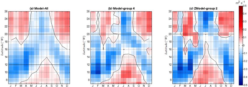
2724                                    J. Mignot et al.: Towards an objective assessment of climate multi-model ensembles

However, the number of general circulation models (GCMs)            al., 2019). Sylla et al. (2019) have recently shown that the
available for climate change projections is increasing rapidly.     intensity of the sea surface temperature (SST) seasonal cy-
For example, the CMIP5 archive (Taylor et al., 2012), which         cle along the coasts of Senegal and Mauritania was a good
was used for the fifth IPCC Assessment Report (Stocker et           marker of the upwelling in this specific region in climate
al., 2013), contains outputs from 61 different GCMs, and 70         models. They have used this index together with other more
contributions are expected for CMIP6. It thus becomes pos-          dynamical indices to predict that the upwelling will decrease
sible – and probably necessary – to select and/or weight the        by about 10 % of its present-day amplitude by the end of
models constituting such an average. Recent work has sug-           the 21st century. Nevertheless, their study also highlighted
gested that weighting the multi-model averaging procedure           a large uncertainty due to model biases in this region. The
could help to reduce the spread and thus uncertainty of fu-         method we have developed selects a subset of the CMIP5
ture projections. Such an approach has been applied exten-          ensemble based on the capability of the climate models to
sively to the issue of climate sensitivity (Fasullo and Tren-       reproduce the SST seasonal cycle observed during the histor-
berth, 2012; Gordon et al., 2013; Huber and Knutti, 2012;           ical period in key sub-regions. These sub-regions are identi-
Tan et al., 2016). Valuable improvement of model selection          fied by a neural classifier. The method leads us to rank the
has also been found in studies of the carbon cycle (Cox et al.,     different models and to determine an efficient multi-model
2013; Wenzel et al., 2014), the hydrological cycle (Deange-         combination for the analysis of the Senegalo-Mauritanian
lis et al., 2015; O’Gorman et al., 2012), the Antarctic atmo-       upwelling and projections of its behavior in global warming
spheric circulation (Son et al., 2010; Wenzel et al., 2016), ex-    conditions.
tratropical atmospheric rivers (Gao et al., 2016), atmospheric         The paper is structured as follows: Sect. 2 presents the
and ocean heat transports (Loeb et al., 2015), European tem-        different climate models and the climatological observations
perature variability (Stegehuis et al., 2013) and temperature       used in the study, together with the region of interest. The
extremes (Borodina et al., 2017).                                   classification method is described in Sect. 3 and applied to
   The present paper works towards the elaboration of an            the extended region. Section 4 presents a qualitative anal-
objective method to select models according to their per-           ysis able to group the different climate models into clus-
formance for a specific phenomenon. Here, we use the                ters presenting similar performances. Section 5 investigates
Senegalo-Mauritanian upwelling area as a case study to con-         the results of the method applied over a smaller area, more
struct an efficient climate multi-model combination together        focused over the upwelling region. Section 6 uses the two
with its related confidence interval in order to anticipate the     multi-model clusters defined in Sects. 4 and 5, respectively,
effect of climate warming by the end of the century in this re-     to tentatively predict the representation of the Senegalo-
gion. The Senegalo-Mauritanian upwelling has been the fo-           Mauritanian upwelling changes under global warming. Con-
cus of increasing attention over recent years. The very pro-        clusions are given in Sect. 7.
ductive waters associated with the upwelling have a strong
economic impact on fisheries in Senegal and Mauritania and
a crucial societal importance for local populations. It is there-   2     Climate models and region of interest
fore important to predict the evolution of the dynamics and
the physics of the upwelling in the forthcoming decades,            2.1    Data
due to the effect of climate warming and its consequences
for biological productivity, which may impact the fisheries.        This study is based on the CMIP5 (Coupled Model Inter-
The Senegalo-Mauritanian upwelling lies at the southern end         comparison Project Phase 5) database. We use the output of
of the Canarian upwelling system, which has a relatively            47 simulations listed in Table 1. The models are evaluated
weak seasonality and is maximum in summer. By contrast,             over the historical period defined as [1975–2005] by com-
the Senegalo-Mauritanian upwelling presents a well-marked           paring their output to observations. The mean seasonal cy-
seasonal variability. Its intensity is stronger in boreal win-      cle of SST anomalies over this period is constructed for each
ter, and it disappears in summer with the northward progres-        model grid point as the difference between the monthly mean
sion of the intertropical convergence zone (ITCZ). Due to           temperature and the mean annual temperature. When several
the enrichment of the sea surface layers with nutrients up-         members of historical simulations are available for a spe-
welled from deep layers, it drives an important phytoplank-         cific model configuration, they are averaged together. How-
ton bloom that is observed on ocean color satellite images          ever, this has practically no impact on the estimated mean
(Demarcq and Faure, 2000; Farikou et al., 2015). The maxi-          seasonal cycle (not shown). The mean climatological cycle
mum intensity of this bloom occurs in March–April (Farikou          of the CMIP5 models under study is evaluated against the
et al., 2015; Faye et al., 2015; Ndoye et al., 2014). Its im-       Extended Reconstructed Sea Surface Temperature data set
portant seasonal cycle is also associated with mesoscale pat-       (ERSST-v3b, Smith et al., 2008), averaged over the same
terns whose variability has been recently studied by several        time period. This data set was produced by NOAA at 2◦ spa-
oceanographic campaigns (Capet et al., 2017; Faye et al.,           tial resolution. It is derived from the International Compre-
2015; Ndoye et al., 2014) and theoretical work (Sirven et           hensive Ocean–Atmosphere Dataset with missing data filled

Geosci. Model Dev., 13, 2723–2742, 2020                                              https://doi.org/10.5194/gmd-13-2723-2020
J. Mignot et al.: Towards an objective assessment of climate multi-model ensembles                                              2725

Table 1. List of the CMIP5 models used for the comparison. The       2.2    The Senegalo-Mauritanian upwelling region
reader is referred to the CMIP5 documentation for more information
on each of them. Here, each configuration is furthermore given a     In this study, we evaluate the ability of the different climate
number, for easier identification in subsequent figures.             models to represent the Senegalo-Mauritanian upwelling.
                                                                     Following Sylla et al. (2019), we consider the intensity of the
  nb   Model acronym               nb    Model acronym               seasonal cycle of the SST anomaly to be a marker of the up-
  1    bcc-csm1-1                  25    HadGEM2-ES                  welling variability and localization. This variable is shown in
  2    bcc-csm1-1-m                26    MPI-ESM-LR                  Fig. 1 for the eastern tropical Atlantic. This figure confirms
  3    BNU-ESM                     27    MPI-ESM-MR                  that the Senegalo-Mauritanian coast stands out with a very
  4    CanCM4                      28    MPI-ESM-P                   strong seasonal SST cycle as compared to similar latitudes
  5    CanESM2                     29    MRI-CGCM3                   in the open ocean. This results from the cold SST gener-
  6    CMCC-CESM                   30    MRI-ESM1                    ated by the strong winds occurring in winter. The Senegalo-
  7    CMCC-CM                     31    GISS-E2-H
                                                                     Mauritanian upwelling is confined in a small region on the
  8    CMCC-CMS                    32    GISS-E2-H-CC
  9    CNRM-CM5                    33    GISS-E2-R
                                                                     order of 100 km off the western coast of Africa. It is part of a
  10   CNRM-CM5-2                  34    GISS-E2-R-CC                complex and fine-scale regional circulation system recently
  11   ACCESS1-0                   35    CCSM4                       revisited by Kounta et al. (2018). Since the grid mesh of most
  12   ACCESS1-3                   36    NorESM1-M                   of the climate models is on the order of 1◦ (∼ 100 km), this
  13   CSIRO-Mk3-6-0               37    NorESM1-ME                  regional circulation is poorly resolved, which favors a rel-
  14   inmcm4                      38    HadGEM2-AO                  atively large-scale analysis of the upwelling representation
  15   IPSL-CM5A-LR                39    GFDL-CM2p1                  in climate models. The Senegalo-Mauritanian upwelling is
  16   IPSL-CM5A-MR                40    GFDL-CM3                    also embedded in a large-scale oceanic circulation pattern,
  17   IPSL-CM5B-LR                41    GFDL-ESM2G
                                                                     encompassing the North Equatorial Counter Current flow-
  18   FGOALS-g2                   42    GFDL-ESM2M
  19   FGOALS-s2                   43    CESM1-BGC                   ing eastward in the southern part of the region and the re-
  20   MIROC-ESM                   44    CESM1-CAM5                  turn branch of the subtropical gyre in the northwestern part.
  21   MIROC-ESM-CHEM              45    CESM1-CAM5-1-FV2            Therefore, we firstly study the representation of the SST sea-
  22   MIROC5                      46    CESM1-FASTCHEM              sonal cycle intensity in the different climate models over a
  23   HadCM3                      47    CESM1-WACCM                 relatively large region that includes part of the Canary Cur-
  24   HadGEM2-CC                                                    rent in the north and the Guinea Dome in the south. The so-
                                                                     called “extended region” is defined by a rectangular box ex-
                                                                     tending from 9 to 45◦ W and from 5 to 30◦ N (Fig. 1). In a
in by statistical methods. This data set is used as the target to    second step, we will proceed to the same analysis and classi-
be reproduced and is denoted “observation field” hereafter.          fication of the models within a much more focused (hereafter
In order to deal with data at the same resolution, all model         zoomed) region, namely [16–28◦ W and 10–23◦ N] (Fig. 1).
outputs as well as the observation fields were regridded on a        All the results below will be first shown for the extended re-
1◦ resolution regular grid prior to analysis. A previous study       gion. Comparison with the focused region will be done in
(Sylla et al., 2019) has compared the performance of this data       Sect. 4.
set as compared to the gridded SST data set from the Met
Office Hadley Centre HadISST (Rayner, 2003). The main re-
sults regarding the future of the upwelling were shown to be         3     Comparing observations and models: a
independent of the validation data set, primarily because the              methodological approach
models’ biases and the inter-model differences were much
larger than the differences between the validation data sets.        The methodology we have developed is based on the ability
The methodological and oceanographic results presented in            of the climate models to adequately reproduce the climatol-
this study are thus expected to depend only very weakly on           ogy of the seasonal cycle of the SST anomalies as observed
the target data set.                                                 during the last 3 decades in key sub-regions of the studied
   In Sect. 6, the model selections are used to characterize         domain. These key sub-regions are determined from the sim-
the response of the upwelling to climate change. This re-            ilarity of their physical and statistical characteristics through
sponse is characterized in terms of SST anomalies as well as         an unsupervised classification, which clusters pixels with
wind intensity. For wind intensity, the simulated wind stress        similar observed seasonal SST climatology. We chose to deal
is compared to the TropFlux reanalysis. This data set com-           with a neural classifier, the so-called self-organizing map
bines the ERA-Interim reanalysis for turbulent and longwave          (SOM hereafter) developed by Kohonen (2013), followed by
fluxes and ISCCP (International Satellite Cloud Climatol-            a hierarchical ascendant clustering (HAC, Jain and Dubes,
ogy Project) surface radiation data for shortwave fluxes. This       1998). This method leads to a dynamically interpretable clas-
wind stress product is described and evaluated in Praveen            sification. The SOM determines a vector quantization of the
Kumar et al. (2011).                                                 data set, which compresses the initial data set into a rela-

https://doi.org/10.5194/gmd-13-2723-2020                                               Geosci. Model Dev., 13, 2723–2742, 2020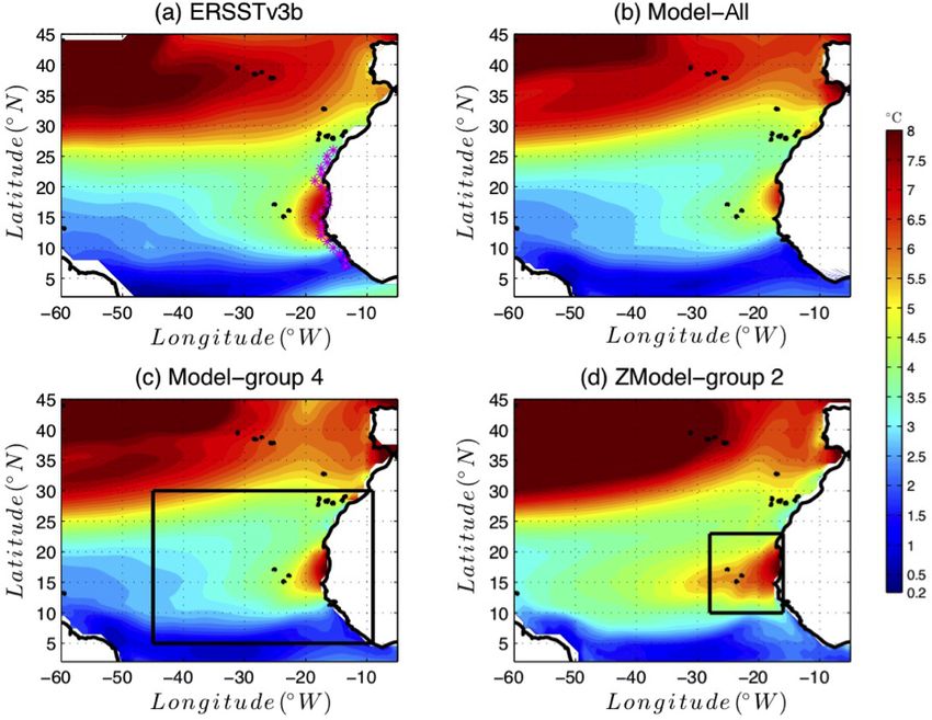
2726                                     J. Mignot et al.: Towards an objective assessment of climate multi-model ensembles

                                                                      gular grid. This graphical structure is used to define a dis-
                                                                      crete distance (denoted by δ) between the neurons of the map
                                                                      and thereby identify the shortest path between two neurons.
                                                                      Moreover, the SOM enables the partition of D in which each
                                                                      cluster is associated with a neuron of the map and is rep-
                                                                      resented by a prototype that is a synthetic multidimensional
                                                                      vector (the referent vector w). Each vector z of D is assigned
                                                                      to the neuron whose referent w is the closest, in the sense of
                                                                      the Euclidean norm (EN), and is called the projection of the
                                                                      vector z onto the map. A fundamental property of a SOM is
                                                                      the topological ordering provided at the end of the clustering
                                                                      phase: two neurons that are close on the map represent data
                                                                      that are close in the data space. In other words, the neurons
                                                                      are gathered in such a way that if two vectors of D are pro-
                                                                      jected onto two “relatively” close neurons (with respect to δ)
                                                                      on the map, they are similar and share the same properties.
Figure 1. Amplitude of the SST seasonal anomalies in the western      The estimation of the referent vectors w of a SOM and the
tropical North Atlantic. SST data are from the ERSSTv3b data set
                                                                      topological order is achieved through a minimization process
averaged between 1975 and 2005. The two black boxes show the
                                                                      using a learning dataset base, here from the observations. The
extended and zoomed regions, respectively, on which the statistical
classifications were performed (see text for details).                cost function to be minimized is of the form
                                                                                       X X
                                                                        T
                                                                      JSOM  (χ , W ) =            K T (δ (c, χ (zi )))|zi − wc |2 ,
                                                                                      zi∈D c∈SOM
tively small number of reference vectors. Doing so allows us
to take the nonlinearities of the data set into account and to        where c ∈ SOM indices the neurons of the SOM, χ is the
filter the noise, which can make the classification spurious.         allocation function that assigns each element zi of D to its
This reduced number of dataset vectors enables an HAC to              referent vector wχ(zi ) and δ(cχ (zi )) is the discrete distance
determine the highly nonlinear borders between the different          on the SOM between a neuron c and the neuron allocated
SOM clusters. This procedure has been used with success in            to observation zi . K T a kernel function parameterized by T
several studies (Farikou et al., 2015; Jouini et al., 2016; Ni-       (where T stands for “temperature” in the scientific literature
ang et al., 2003, 2006; Sawadogo et al., 2009). Note that the         dedicated to SOM) that weights the discrete distance on the
use of an HAC directly on the initial data set would not be           map and decreases during the minimization process. At the
efficient in the present study because the number of degrees          end of the learning process, the classification can be visual-
of freedom (here the grid points of the initial domain) is too        ized onto the SOM and interpreted in terms of geophysics.
large for this method to work efficiently. In the present sec-
tion, we describe the methodology we developed to score the           3.2   Classification of the observations
different climate models with respect to the observations. In
Sect. 4, we will tentatively group the different climate mod-         In the present problem we chose to classify the annual cy-
els into blocks with the same behavior by using a multiple            cles of the SST seasonal anomalies observed in the Senegalo-
correspondence analysis (MCA).                                        Mauritanian upwelling. The study was made on the “ex-
                                                                      tended region” constituted of 25 × 36 = 900 pixels, but this
3.1    The unsupervised classification method                         enlarged region covers a part of the African continent, and
                                                                      157 pixels are in fact over land. That means that we have
The first step of the methodology was to decompose the                truly 743 ocean pixels to deal with. We consider a time pe-
selected region into different classes (the key sub-regions           riod of 30 years [1975 to 2005] extracted from the ERSST-
mentioned above) by using a neural network classifier, the            V3b database. For a given grid point and a given year and
so-called SOM (Kohonen, 2013). This algorithm constitutes             month, the monthly anomaly is the SST of the pixel for which
a powerful nonlinear unsupervised classification method. It           we have subtracted the mean of the considered year. The
has been commonly used to solve environmental problems                climatological mean of the anomaly is then computed for
(Hewitson and Crane, 2002; Jouini et al., 2013, 2016; Liu et          each grid point by averaging each climatological month over
al., 2006; Reusch et al., 2007; Richardson et al., 2003). The         the 30 years. Thus, the learning data set D is a set of 743
SOM aims at clustering vectors (here the 12 SST seasonal              12-component vectors z, each component being the mean
anomalies) of a multidimensional database (D) (here the grid          monthly anomaly computed as above. We denote as “SST
points of the studied domain) into classes represented by a           seasonal cycle” the vector z in the following.
fixed network of neurons (the SOM). The SOM is defined                   We used a SOM to summarize the different SST seasonal
as an undirected graph, usually a two-dimensional rectan-             cycles present in the “extended region”. We found that 120

Geosci. Model Dev., 13, 2723–2742, 2020                                               https://doi.org/10.5194/gmd-13-2723-2020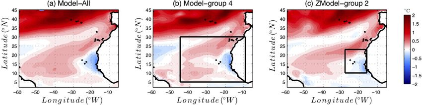
J. Mignot et al.: Towards an objective assessment of climate multi-model ensembles 2727
prototypes (or neurons) can accurately represent the 743 vec- evaluating process. This kind of approach has been proposed
tors of D. This reduction (or vector quantization) is made by in Sylla et al. (2019), and we indeed immediately see that
using a rectangular SOM of 30 × 4 neurons. some models better fit the “observation field” than others.
We then reduced the number of neurons in order to fa- Nonetheless, this method remains very subjective.
cilitate their interpretation in terms of geophysical processes. In the following, we present a more objective approach.
For this, we applied a HAC using the Ward dissimilarity (Jain We use the previous classification to objectively estimate
and Dubes, 1988). We grouped the 120 neurons of the SOM how each CMIP5 model fits the “observation field” and its
into a hierarchy that can contain between 1 and 120 clusters. seven region clusters. For this, we projected the SST annual
Then the different classifications proposed by the HAC were cycle of each CMIP5 model grid point of the extended region
applied to the geographical region: each SST seasonal cy- onto the SOM learned with the observations (Sect. 3.2) using
cle of each grid point of the region is assigned to a neuron the assignment procedure described in this section. Each grid
and consequently to a cluster (assignment process), thereby point thus corresponds to a cluster of the SOM and is repre-
defining the so-called region clusters. The problem is then to sented on the geographical map by its corresponding color.
choose a number of clusters that adequately synthesizes the Doing so, we can represent each CMIP5 model by the geo-
geophysical phenomena over the region. This was done by graphical pattern of the seven clusters partitioning the SST
looking at the different possible classifications and choosing seasonal cycle of its grid points. The geographical maps rep-
one representing the major characteristics of the upwelling resenting the 47 models and their associated clusters are plot-
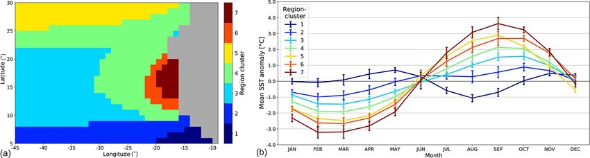
region. In Fig. 2a, we observe that when we partition the ted in Fig. 3. This graphical visualization is easier to compare
SOM into seven clusters, the associated seven region clusters than the original characteristics (amplitude and phase) of the
are constituted of contiguous pixels in the geographic map annual cycle at each grid point of a model since each grid
and that two clusters (6, 7) are within the upwelling region point can only take one discrete value among seven. This rep-
and present a well-marked seasonal cycle. For each region resentation immediately allows identification of the model
cluster, we estimated the monthly mean of the SST seasonal biases and the models that best reproduce the cluster regions
cycle and the associated spread captured by the neurons con- identified in the observations. A huge amount of information
stituting this region cluster. could in principle be extracted from these maps, both from
The typical SST climatological cycles for each region individual modeling groups, to understand the representation
cluster are presented in Fig. 2b together with their related of this region by the models and the origins of possible bi-
error bars. We note that the region clusters are well identi- ases, and from experts of the area, to understand the difficul-
fied, their typical climatological annual cycles of SST be- ties of the climate models in representing the SST seasonal
ing well separated. Furthermore, the seven region clusters cycle in this region.
are spatially coherent and have a definite geophysical sig- For a more quantitative assessment, we counted the num-
nificance. ber of grid points of a region cluster for a given CMIP5 model
For the extended region under study, 7 therefore appears matching the same region cluster of the “observation field”.
to be an adequate cluster number, since this number balances We then computed the ratio between that matching number
a clear partition of the clusters on the HAC decision tree and the number of pixels of the region cluster of the consid-
with a clear physical significance to each region cluster. The ered model. That number is noted in the color bar for each re-
Senegalo-Mauritanian coastal upwelling is associated with gion cluster in Fig. 3. We denote Rm,i the ratio for the region
clusters 7 and 6. Cluster 2 corresponds to deep tropical wa- cluster i and the model m, where i = 1, . . ., 7 is the number
ters associated with the equatorial countercurrent. Cluster 1 of the region cluster and m = 1, . . ., 47 is the number of the
corresponds to surface waters of the Gulf of Guinea. Cluster model (see Table 1). We note that Rm,i ≤ 1. Doing so, each
3 corresponds to the offshore tropical Atlantic, and cluster 5 model m is represented by a seven-dimensional vector Rm ,
has extratropical characteristics. Cluster 4 is a transition be- each component being the ratio of a region cluster. We esti-
tween 3 and 5. As expected, the equatorial regions (clusters mated the total skill of a model by averaging the seven ratios.
1 and 2) have a very weak seasonal cycle, which increases Note that this procedure gives the same weight to each re-
towards the extratropics (clusters 3 to 5). The upwelling re- gion cluster whatever its number of grid points and its prox-
gions (clusters 6 and 7) are characterized by an exceptionally imity to the upwelling region. In the following, the skill is
strong seasonal variability. presented as a percentage: the higher the skill, the better the
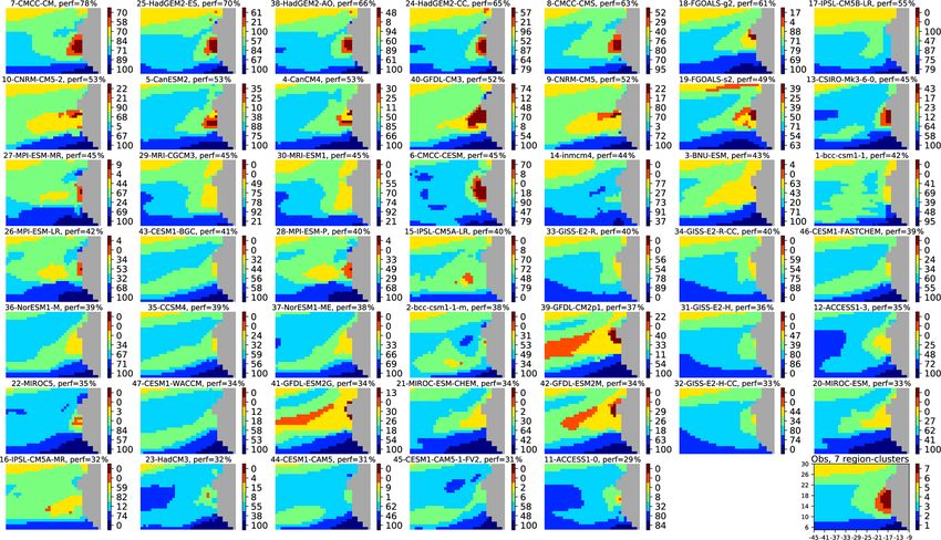
fit. In Fig. 3, the 47 CMIP5 models are ranked by their total
3.3 Classification of the climate models on the extended skill, which is indicated above each panel beside the model
upwelling region name. The model skills are very diverse, ranging from 79 %
to 28 %. This figure also shows that the models presenting the
The aim is now to find the model(s) that best fit the “obser- best total skill are also those representing thoroughly the up-
vation field”. A heuristic manner is to compare the pattern welling region. Some models represent the large-scale struc-
of the different region clusters of the CMIP5 models with ture in the eastern tropical Atlantic (Region-clusters 3, 4, and
respect to those of the “observation field” through a sight- 5) very well, but not the upwelling (33-GISS-E2-R and 34-
https://doi.org/10.5194/gmd-13-2723-2020 Geosci. Model Dev., 13, 2723–2742, 2020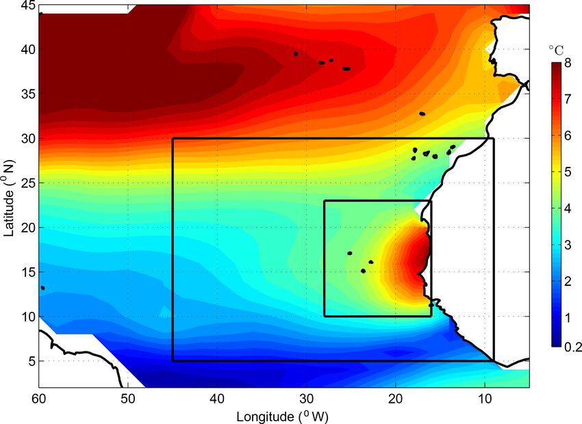
2728                                      J. Mignot et al.: Towards an objective assessment of climate multi-model ensembles

Figure 2. (a) Region clusters associated with the SOM clusters obtained after a HAC on a 30 × 4-neuron SOM learned on ERSSTv3b
observations in the extended zone (see text for details). (b) Ensemble-mean monthly climatological SST anomalies for the grid points of the
seven region clusters. The error bars show the standard deviation of this ensemble mean.

Figure 3. Projection of the 47 climate models of the CMIP5 database onto the SOM learned with ERSSTv3b climatology in the extended
zone (see Fig. 1). On top of each panel, we figure the number referencing the model, its name (Table 1), and its skill given as a mean
percentage (see text). The models are ordered according to their skill in decreasing order. The seven region clusters (or SOM clusters) are
defined by applying an HAC to the SOM output learned with the observation field. They are represented by different colors. The numbers in
the color bar on the right of each panel represent the skill for each region cluster. The observation field is shown in the bottom right panel
and the numbers in front of the color bar reference the region cluster.

GISS-E2-R-CC, for example). Others represent pretty well                 sonality of the SST cycle in each of the models, potentially
the upwelling region clusters (Region-clusters 6 and 7), but             a very useful guide for climate modelers to identify rapidly
not the large-scale structures of the SST seasonality (13-               major biases.
CSIRO-Mk-3-6-0 and 6-CMCC-CESM, for example). None
of these models is ranked among the best models, with a
score greater than 60 %. As indicated above, this represen-
tation gives a very synthetic view of the structure of the sea-

Geosci. Model Dev., 13, 2723–2742, 2020                                                    https://doi.org/10.5194/gmd-13-2723-2020
J. Mignot et al.: Towards an objective assessment of climate multi-model ensembles                                           2729

4   Qualitative analysis of the climate models                    allows understanding of the drawback of the different models
                                                                  with respect to the seven modes of SST cycles.
                                                                     As indicated in the introduction, the main objective of the
In order to further progress in the selection of the models,      methodology is to select an ensemble of models that repre-
the 47 climate models and the observation field were then         sents at best the upwelling behavior with respect to the ob-
analyzed by using an MCA. MCA is a multivariate statistical       servations and to use this ensemble to predict the impact of
technique that is conceptually similar to principal component     climate change on the Senegalo-Mauritanian upwelling with
analysis (PCA) but applies to categorical rather than contin-     some confidence. The problem is now to determine a sub-
uous data. Similarly to PCA, it provides a way of displaying      set of models which has a better skill than Model-All, in
a set of data in a two-dimensional graphical form.                other words minimize the distance to the observations. As
   In the following, we apply a MCA to the (47, 7) matrix         the number of models is small enough, we chose to cluster
R = [Rm,i ] whose elements represent the skills of the clus-      them by an HAC according to their projections onto the six
ters of the models shown in front of the color bars in Fig. 3:    axes provided by the MCA and select the optimal jump in
the rows m represent the 47 different models, the columns i       the hierarchical tree (Jain and Dubes, 1988). We recall that
the seven region clusters. The MCA, like the PCA, projects        the HAC (hierarchical ascending clustering) is a bottom–up
the initial matrix onto a new basis in such a way that the        algorithm for dataset clustering. The key operation in hierar-
new axes are the matrix eigenvectors (PC), the inertia of each    chical bottom–up clustering is to repeatedly combine the two
axis being the corresponding eigenvalues. According to the        nearest (according to a certain distance) clusters into a larger
theory, the MCA matrix analysis of R gives i − 1 = 6 inde-        cluster. The HAC starts from individuals and combines them
pendent PCs. Each model is thus now associated with a six-        according to their similarity (with respect to the chosen dis-
dimensional vector on which it has a specific weight. The         tance) to obtain new clusters. The process is repeated up to
MCA uses for this analysis the χ 2 distance. In Fig. 4, we        get one cluster only (the full data set). This algorithm is visu-
present the projection of the models and the “region clus-        alized through a tree-like diagram, the so-called connection
ters” in the plane formed by the two first axes (x = PC1 and      tree or dendrogram: the branches of the connection tree rep-
y = PC2) of the MCA. These two axes represent 70 % of the         resent the connections between the clusters (Fig. 5). From
total inertia. Each model is represented by a small circle and    Fig. 5, we obtain four homogeneous groups which are well
each region cluster by a purple square. We also projected the     separated (group 1, 2, 3, and 4). They are plotted with differ-
observation field (green diamond) onto that plane. To have a      ent colors in Fig. 4. We denote as Model-group 1, Model-
more precise view of the topology, it would be necessary to       group 2, Model-group 3, and Model-group 4 these multi-
consider the projection onto the five other PCs, which repre-     model ensembles hereafter. Note that Fig. 4 shows the pro-
sent 30 % of the inertia.                                         jection of the individual models onto the first two axes of the
   In the (PC1, PC2) plane, the shorter the distance between      MCA. The fact that only two axes are shown here can intro-
two models, the more similar the distribution of their region-    duce some bias into the visualization, and this figure must be
cluster skills. Proximity between a model and a region cluster    considered with some caution.
leads us to affirm that this region cluster is well represented      Through MCA+HAC, we thus grouped the models into
by that model. Clearly, some models adequately represent the      clusters, using the χ 2 distance, according to their proxim-
southern part of the extended region (Region-clusters 1, 2 or     ity to the observations and their internal similarity. For each
3), where the SST seasonal cycle is weak, and are very distant    group, we computed a multi-model average whose outputs
from the upwelling regions (Region-cluster 6 and Region-          are the mean of the outputs of its different members, and we
cluster 7) whose large SST cycle is poorly reproduced. In this    analyzed it according to the same procedure (projection of
group of models, one recognizes the model 16-IPSL-CM5A-           the SST seasonal cycle and assignment to a region cluster)
MR, at the extreme bottom of Fig. 4, close to Region-clusters     used for each individual model. In addition, we introduced
4 and 5, consistently with Fig. 3. At the other end of this       the full multi-model average (Model-All in the following),
group of models, model 23-HadCM3 for example is located           which is the multi-model ensemble, which averages the 47
very close to Region-cluster 1. Figure 3 indeed shows that        CMIP5 model outputs. Model-All was also projected in the
most of its grid points over the region of interest have a sea-   MCA plane, and it is represented by a red star in Fig. 4.
sonal cycle resembling the one found in the offshore tropical     Comparison of the four model groups with Model-All and
ocean. Another group of models is located in the center of        the observations are presented in Fig. 6. This figure visually
this plan, thus at an optimal distance of each of the observed    highlights the dominance of Model-group 4 for the recon-
region clusters, and not far from the overall position of the     struction of the SST seasonal cycles of the different region
observations (diamond). We recognize in this group of mod-        clusters for the extended region. This is particularly clear for
els those that have a high skill in Fig. 3. The positioning of    Region-clusters 6 and 7, which are those located in the up-
the observations (green diamond in Fig. 4) with respect to        welling region (Fig. 2). Model-group 3 seems to group mod-
the models indeed allows selection of those that best repre-      els characterized by an equatorward shift of the main struc-
sent the observation field. The representation given in Fig. 4    tures, since Region-cluster 1 of tropical waters is not repro-

https://doi.org/10.5194/gmd-13-2723-2020                                            Geosci. Model Dev., 13, 2723–2742, 2020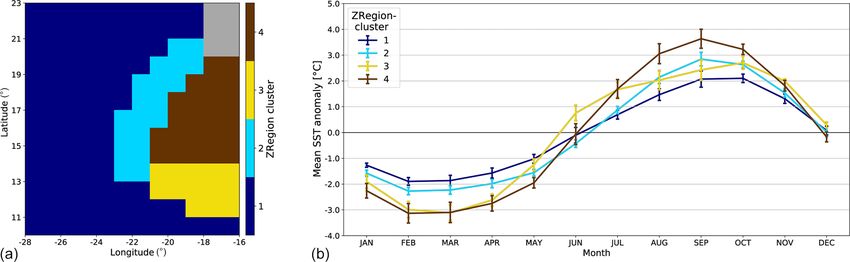
2730                                      J. Mignot et al.: Towards an objective assessment of climate multi-model ensembles

Figure 4. Projection of the CMIP5 models (colored circles) and the observation field (green diamond) defined by their cluster skill vectors
onto the first two axes of the MCA. The seven region clusters of the observation field are represented by purple squares. The colors of the
circles denote the four groups of models obtained after an HAC was performed on the seven MCA components of the models. The projection
of the full multi-model mean (47 models) is represented by a red star. We note that some bias can be introduced into this projection since the
projection onto the other axes can be of importance.

duced and Region-clusters 4 and 5 of extratropical waters are            and model 25) and to outline the best multi-model (Model-
overestimated. Figure 4 indeed shows that this model group               group 4) whose skill is better than any model with a proba-
is very close to Region-clusters 4 and 5, which correspond to            bility of 95 % (number of models whose skill is smaller than
the extratropical and transition geographical regions. Model-            the skill of Model-group 4 with respect to the total number
group 2 misrepresents the region of the Canary upwelling.                of models). Projection of the models onto the other planes
Model-group 1 overestimates the SST seasonal cycle in all                of the MCA should confirm this interpretation. One could
the tropical open Atlantic. These two last model groups over-            then question the use of Model-group 4 rather than model 7
estimate Region-cluster 1, again consistently with their posi-           or model 25 individually. Furthermore, we argue that multi-
tion in Fig. 4. A detailed physical interpretation of the model          model averages are in general more robust for climate stud-
groups is nevertheless beyond the scope of this paper. Clearly           ies than the use of a single model that can have good per-
Model-All represents the SST seasonal cycle of the offshore              formance for a very specific set of constraints but not for
ocean, but it proposes a very poor representation of the up-             neighboring ones. The following section will partly justify
welling region.                                                          this point.
   Two models (models 7 and 25) have a better skill than
Model-group 4 and Model-All. These two models are very
close to the observations on the first two axes of the MCA
                                                                         5    Analysis of the climate models over a zoomed
(Fig. 4). It is easily seen that Model-group 4 and the pro-
                                                                              upwelling region
jection of Model-All onto this plane are farther than that of
model 7 and model 25 from the observation projection. This
                                                                         The classification presented above relies largely on the abil-
explains the lower performance of these two multi-models
                                                                         ity of the models to represent the offshore seasonal cycle of
as compared to models 7 and 25. In the present case, the
                                                                         the SST. In the following, we propose to test the classification
method permits one to determine the best models (model 7
                                                                         over a much more reduced area in order to focus the analy-

Geosci. Model Dev., 13, 2723–2742, 2020                                                    https://doi.org/10.5194/gmd-13-2723-2020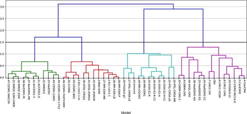
J. Mignot et al.: Towards an objective assessment of climate multi-model ensembles                                                         2731

Figure 5. HAC dendrogram. The horizontal line displays the 47 CMIP5 models, each model being associated with its seven-component skill
vector. As the dendrogram represents a hierarchy of clusters, the numbers on the y axis give the distance between two clusters. We note an
optimal “jump” on this graph: the level 1.5 on the vertical axis (materialized by a horizontal black line) is associated with four well-separated
clusters corresponding to four model groups that are very different.

Figure 6. (a–d) Projection of the multi-model ensembles (model group) onto the SOM learned with ERSSTv3b climatology in the extended
zone. Multi-model ensemble performances are obtained by averaging the skill of the models forming each group. The performances are given
on top of each panel. The region clusters determined by processing the observations in the extended area and their associated colors are given
in panel (f). The color bars at the right of each multi-ensemble panel represent the skill (in %) associated with each region cluster. Panel
(e) shows the projection for the full multi-model ensemble. Panel (f) reproduces the region clusters based on the observations also shown in
Fig. 2.

sis on the upwelling area. This “zoomed upwelling region”                  new MCA to regroup the climate models. We did a simi-
is shown in Fig. 1.                                                        lar analysis to that performed in Sect. 4. We obtained four
   As for the extended region, we partitioned the observa-                 new well-separated region clusters denoted ZRegion clus-
tions of the zoomed upwelling region with a SOM (ZSOM                      ters. Figure 7 shows the four ZRegion clusters obtained
in the following) followed by a HAC. We then applied a                     from ERSSTv3b observations together with their associ-

https://doi.org/10.5194/gmd-13-2723-2020                                                       Geosci. Model Dev., 13, 2723–2742, 2020
2732                                   J. Mignot et al.: Towards an objective assessment of climate multi-model ensembles

ated mean SST seasonal cycle. Again, the ZRegion clus-             characterizes ZModel-groups 3 and 4. ZModel-group 5 cor-
ters are spatially coherent. The upwelling area is now de-         responds to a shift of the upwelling region towards the north.
composed into three ZRegion clusters (ZRegion-clusters 2,          Model-All also shows a strongly reduced seasonal cycle,
3, and 4). This new decomposition thus refines the study           with a large number of pixels in the intermediate ZRegion-
performed for the extended region: ZRegion-cluster 1 repre-        cluster 3 and very few in ZRegion-cluster 4. ZRegion cluster
sents the offshore ocean; its grid points typically have a SST     3, representing the southern part of the Senegalo-Mauritanian
seasonal cycle amplitude of 4 ◦ C, very similar to Region-         upwelling, does not appear in the pattern of Model-All.
cluster 4 in the classification performed over the extended            It is notable that all the models forming ZModel-group 2
region (Fig. 2). ZRegion-cluster 4 identifies the core of the      are included in Model-group 4. For a more precise assess-
Senegalo-Mauritanian region, with grid points characterized        ment, we can also project the entire Model-group 4, iden-
by the greatest amplitude of the SST seasonal cycle of the         tified as the best multi-model ensemble over the extended
domain, typically 6.5 ◦ C. It is interesting to note that an ad-   region, onto the ZSOM (Fig. 9b). We notice that the per-
ditional upwelling ZRegion cluster (ZRegion-cluster 3) ap-         formance of Model-group 4 remains high on this projec-
pears south of ZRegion-cluster 4. Indeed, several studies          tion, indicating some robustness of this multi-model ensem-
have shown that the Cape Verde peninsula, located around           ble. Moreover, this ensemble now outperforms the single best
15◦ N, separates the upwelling region into two distinct areas      model identified over the extended region (Fig. 9a). This re-
with a different behavior north and south of this peninsula        sult gives further confidence in the use of multi-model av-
(Sirven et al., 2019; Sylla et al., 2019). The location of the     erages, illustrating that one single model can be very skill-
separation between ZRegion-clusters 3 and 4 is determined          ful over a specific region or for a specific analysis, but
with some uncertainty due to the coarse resolution (1◦ ) of the    multi-model averages are more robust across various anal-
ocean models. ZRegion-cluster 3 is marked by a time shift          yses and/or regions.
of the seasonal cycle: the warmest season seems to occur
approximately 1 month earlier than in the other regions, as
clearly seen in Fig. 7a (yellow curve in June). Due to a clas-     6     Impact of climate change on the
sification using a much larger region, such a characteristic             Senegalo-Mauritanian upwelling
does not appear in the extended area study. The physical in-
terpretation of the SST seasonal cycle of this ZRegion cluster     6.1    Representation of the upwelling in the CMIP5
is beyond the scope of the present study, but one can suspect             climate model clusters
a role of the ITCZ seasonal migration covering these grid
points earlier than further north. Finally, ZRegion-cluster 2 is   In this section, we compare the representation of the
a transition between the large-scale ocean and the upwelling       Senegalo-Mauritanian upwelling system given by the two
region.                                                            best model groups identified above (model group 4 and
   As for the extended region, we applied a MCA to the             ZModel group 2). For this evaluation, we use two of the
(47 × 4) matrix R = [Rm,i ] whose elements represent the           five indices used by Sylla et al. (2019) to evaluate the full
skills of the four clusters (i) of the 47 models. This MCA         database, namely the intensity of the SST seasonal cycle and
was followed by a HAC leading the definition of five ZModel        the offshore Ekman transport at the coast. The former is spe-
groups. The members of each group are given in the Ap-             cific to the seasonal variability of the Senegalo-Mauritanian
pendix. Figure 8 shows the ZRegion cluster obtained in             upwelling system, and it has been used for the classification.
the zoomed area by projecting these five ZModel groups             The latter is more general and, although it has recently been
and Model-All onto the ZSOM and their associated perfor-           shown to partly represent the volume of the upwelled waters
mances. ZModel-group 1 is the worst performing one: only           (Jacox et al., 2018), it is extensively used in the scientific
25 % of the grid cells fall into the same class as for the ob-     literature to characterize upwelling regions (Cropper et al.,
servations. The structure of this model group shows that it is     2014; Rykaczewski et al., 2015; Wang et al., 2015). Note also
characterized by a homogeneous amplitude of the seasonal           that, following Sylla et al. (2019), evaluation is performed on
cycle over the whole domain, suggesting a largely reduced          the period [1985–2005]. This period slightly differs from the
upwelling: only one grid point at the coast has an enhanced        classification period, but the SST seasonal cycle is not sig-
SST seasonal cycle as compared to the large-scale tropical         nificantly different (not shown).
ocean. ZModel-group 2 is the best performing one: 66 %                Figure 10 compares the amplitude of the SST seasonal
of the grid points are assigned to the correct class and the       cycle as represented in the observations, Model-All, Model-
general picture indeed represents a four-class picture fairly      group 4 and ZModel-group 2 identified above. Consistently
consistent with the observed structure (Fig. 7). Important bi-     with Figs. 6 and 8, Model-All dramatically underestimates
ases yet remain. In particular, ZRegion-clusters 2 and 4 char-     the upwelling signature in terms of the SST seasonal cycle as
acterizing the upwelling extend too far offshore. The three        compared to the observations. Model-group 4 and ZModel-
other ZModel groups are intermediate. A relatively reduced         group 2 yield improved results: the area of an enhanced SST
upwelling area, with an underestimated SST seasonal cycle,         seasonal cycle is larger in both latitude and longitude, with

Geosci. Model Dev., 13, 2723–2742, 2020                                            https://doi.org/10.5194/gmd-13-2723-2020
J. Mignot et al.: Towards an objective assessment of climate multi-model ensembles 2733
Figure 7. (a) ZRegion clusters associated with the ZSOM clusters obtained after a HAC on a 10 × 12-neuron SOM learned on ERSSTv3b
observations in the zoomed zone (see text for details). (b) Ensemble-mean monthly climatological SST anomalies for the grid points of the
four ZRegion clusters. The error bars show the standard deviation of this ensemble mean.
Figure 8. (a–e) Projection of the multi-model ensembles (ZModel groups) onto the ZSOM. The performances are given on top of each panel.
The ZRegion clusters determined by processing the observations in the zoomed region and their associated colors are given in panel (g). The
color bars at the right of each multi-ensemble panel represent the skill (in %) associated with each ZRegion cluster. Panel (f) shows the same
for the full multi-model ensemble. Panel (g) reproduces the region clusters based on the observations also shown in Fig. 6.
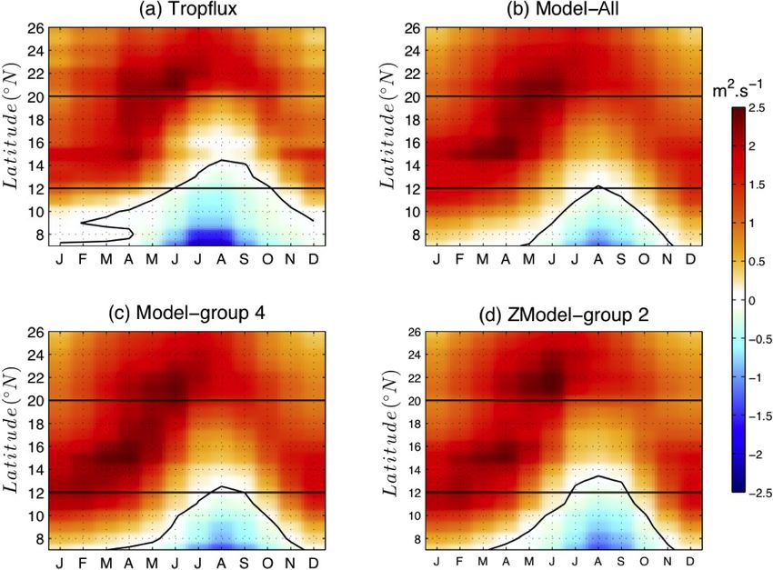
stronger SST amplitude values. This confirms the efficiency The intensity of the wind stress parallel to the coast, induc-
of the selection operated above. Nevertheless, ZModel-group ing offshore Ekman transport and consequently an Ekman
2 yields a realistic SST amplitude pattern along the coast, but pumping at the coast, is generally considered to be the main
it extends too far offshore. Furthermore, in ZModel-group 2, driver of the upwelling. We therefore also tested the represen-
the subtropical area (in green in Fig. 10) extends too far to- tation of this driver in the different model groups. The idea
wards the south, in particular in the western part of the basin. is to evaluate the impact of the model selection performed
The tropical area, characterized by limited amplitude of the above on the representation of an independent variable by the
seasonal cycle of SST (deep blue in Fig. 10), is shifted to the model groups. Figure 11 shows the latitude–time evolution
south as compared to the observations. In other words, the of the meridional oceanic wind stress, considering that the
large-scale thermal – and thus probably dynamical – struc- coast in the studied region is oriented approximately merid-
ture of the region is poorly represented in ZModel-group 2. ionally, so that the offshore Ekman transport is mainly zonal.
Finally, Model-group 4 is the least biased one. Note that in Fig. 11, southward winds have positive values,
so that they correspond to a westward Ekman transport fa-
https://doi.org/10.5194/gmd-13-2723-2020 Geosci. Model Dev., 13, 2723–2742, 20202734 J. Mignot et al.: Towards an objective assessment of climate multi-model ensembles Figure 9. Same as Fig. 7 but for the individual model CMCC-CM (model 7) (a) and model group 4 (b). Figure 10. Amplitude of the SST seasonal cycle in (a) ERSSTv3b observations (b) Model-All, (c) Model-group 4 (best model group for the extended area, illustrated by the black rectangular box) and (d) ZModel-group 2 (best model group for the reduced area, illustrated by the small black rectangular box). The SST seasonal cycle is computed over the period 1985–2005. vorable to upwelling. Panel a shows that the observed merid- The main bias of Model-All (Fig. 11b) is due to the fact that ional wind stress is, all year long, favorable to the upwelling the wind stress never reverses between 12 and 20◦ N. It weak- north of 20◦ N. At these latitudes, the meridional wind stress ens in the southern part of the Senegalo-Mauritanian latitude is stronger in summer. Conversely, between 12 and 20◦ N, in band, i.e., south of the Cape Verde peninsula (15◦ N), but the latitude band of the Senegalo-Mauritanian upwelling, the does not become negative. North of the Cape Verde penin- wind blows southward with a very weak intensity in sum- sula, it also blows from the north in summer, so that the mer, and it even changes direction in the southern part of Senegalo-Mauritanian upwelling lacks seasonality. This bias this latitude band. It is favorable to the upwelling in winter– is corrected in Model-group 4 and ZModel-group 2 (Fig. 11c spring, which explains why the Senegalo-Mauritanian up- and d) that are, in this aspect, more realistic than Model-All. welling occurs during this season with a maximum of inten- Model-group 4 shows a slight extension of the time and lati- sity in March–April (Capet et al., 2017; Farikou et al., 2015). tude range where the oceanic wind stress reverses sign. This Geosci. Model Dev., 13, 2723–2742, 2020 https://doi.org/10.5194/gmd-13-2723-2020
J. Mignot et al.: Towards an objective assessment of climate multi-model ensembles                                          2735

constitutes an improvement. The southward wind is never-             The meridional wind stress also generally weakens under
theless too strong in winter on the [12–20◦ N] latitude band      climate change in the [12–20◦ N] latitude band (Fig. 13), sug-
as well as further south from December to March. These            gesting a general reduction of the upwelling intensity. From
two remaining biases are further reduced in ZModel-group          December to March, this is particularly true in the south-
2. This latter model yields the most realistic seasonal cycle     ernmost region of the Senegalo-Mauritanian band, consis-
of meridional oceanic wind stress on the latitude band under      tent with the results of Sylla et al. (2019). The wind pat-
study. This is consistent with a very localized model selec-      tern inferred from the two model groups (Fig. 13b and c)
tion, as the wind index is itself localized along the coast.      present a higher seasonal variability than those of Model-
   To conclude, Model-group 4 and ZModel-group 2 per-             All (Fig. 13a). The winter reduction of the southward wind
form in general better than Model-All in reproducing the          stress is slightly more confined to the southern region in
major, characteristic features of the Senegalo-Mauritanian        ZModel-group 2, especially at the end of the upwelling
upwelling. This result confirms the relevance of the multi-       season (March–April), when the upwelling intensity is the
model selection we have presented above. Applying the             strongest. This may be consistent with the reduced seasonal
methodology over a relatively large region allows better con-     cycle in the southernmost part of the upwelling identified
straint of the spatial extent and pattern of the SST signature    above.
of the upwelling than the reduced area. The latter however
yields a better representation of the wind seasonality along
the coast.                                                        7   Discussion and conclusion

6.2   Response of the Senegalo-Mauritanian upwelling to           This paper proposed a novel methodology for selecting ef-
      global warming                                              ficient climate models in a specific area with respect to ob-
                                                                  servations and according to well-defined statistical criteria.
In this section, we examine the response of the upwelling         The present study has specifically focused on the ability of
system given by the different multi-model groups we selected      climate models to reproduce the ocean SST annual cycle ob-
to global warming. For this, we compared the two indices          served in specific sub-regions of the studied domain during
analyzed above in present-day and future conditions. The          the period 1975–2005 as reported in the ERSST_v3b data set.
present-day conditions are taken as above as the climatolog-      These sub-regions were defined by a neural classifier (SOM)
ical average of historical simulations over the period [1985–     as clusters with similar seasonal SST cycle anomalies with
2005]. The future period is taken as the climatological av-       respect to some statistical characteristics and were therefore
erage of the RCP8.5 scenario over the period [2080–2100].         named region clusters. They correspond to ocean areas with
Figure 12 shows the difference of the SST seasonal cycle          well-marked oceanographic specificities.
amplitude between these two periods. The general behavior            We then checked the ability of the different climate mod-
is that the SST cycle amplitude will reduce in the upwelling      els to reproduce the region clusters defined on the observa-
region. Sylla et al. (2019) showed that this is primarily due     tion data set with a SOM. The better a climate model fits the
to a warming of the winter temperature, thus suggesting that      clusters computed with the SST observation, the higher the
the upwelling signature at the surface will reduce. On the        skill of the model. To evaluate this, we defined geographical
other hand, this figure shows that the upwelling signature        regions in the different CMIP5 climate models by project-
will increase along the Canary Current, which flows along         ing the SST annual cycle anomalies of each model grid point
the coast of Morocco, as well as in the subtropical part of our   onto the SOM. Each grid point is associated with a cluster
domain. This behavior is observed in the three multi-model        on the SOM and consequently with a region cluster on the
ensembles. However, the two selected model groups suggest         geographical map. We built a similarity criterion by counting
a weaker decrease in the SST seasonal cycle in the upwelling      the number of grid points in a region cluster of a given model
region than the one given by Model-All. ZModel-group 2            matching the same region cluster defined by processing the
shows an even weaker decrease mainly confined in the south-       observation field. We then computed the ratio between that
ern part of the upwelling region. This result echoes findings     matching number and the number of pixels of the region clus-
of Sylla et al. (2019) based on another indicator of the up-      ter of the model under study. We estimated the total skill of
welling imprint on the SST: they showed that the difference       a model by averaging the seven ratios associated with the
between the SST at the coast and offshore is expected to de-      seven region clusters. Note that this procedure presents the
crease more in the southern part of the Senegalo-Mauritanian      advantage of giving the same weight to each region clus-
upwelling system (SMUS) than in the north. We hypothesize         ter whatever its number of grid points and its proximity to
that the study conducted on the reduced area permits sep-         the upwelling region. This procedure respects the clustering
aration of the Senegalo-Mauritanian upwelling system into         done by the SOM since the different clusters have an equal
two clusters, a northern one (ZRegion 4) and a southern one       weight in the skill computation. In its present definition, the
(ZRegion-3) (Fig. 8), which enables us to distinguish this        total skill is a number between 0 and 1: the higher the skill,
specific response.                                                the better the fit. Other measures of the total skill of a model

https://doi.org/10.5194/gmd-13-2723-2020                                            Geosci. Model Dev., 13, 2723–2742, 2020
You can also read