Revisiting Austfonna, Svalbard, with potential field methods - a new characterization of the bed topography and its physical properties
←
→
Page content transcription
If your browser does not render page correctly, please read the page content below
The Cryosphere, 14, 183–197, 2020
https://doi.org/10.5194/tc-14-183-2020
© Author(s) 2020. This work is distributed under
the Creative Commons Attribution 4.0 License.

Revisiting Austfonna, Svalbard, with potential field methods – a new
characterization of the bed topography and its physical properties
Marie-Andrée Dumais1,2 and Marco Brönner1,2
1 Department    of Geoscience and Petroleum, Norwegian University of Science and Technology, 7031 Trondheim, Norway
2 Geological   Survey of Norway, 7040 Trondheim, Norway

Correspondence: Marie-Andrée Dumais (marie-andree.dumais@ngu.no)

Received: 11 April 2019 – Discussion started: 30 April 2019
Revised: 9 August 2019 – Accepted: 14 November 2019 – Published: 22 January 2020

Abstract. With hundreds of metres of ice, the bedrock un-          1   Introduction
derlying Austfonna, the largest icecap on Svalbard, is hard
to characterize in terms of topography and physical proper-
ties. Ground-penetrating radar (GPR) measurements supply           During the last few decades, with satellite technology ad-
ice thickness estimation, but the data quality is temperature      vancement and an increased need to understand climate
dependent, leading to uncertainties. To remedy this, we in-        change, the polar regions have become an important labo-
clude airborne gravity measurements. With a significant den-       ratory for studying ongoing environmental changes. In this
sity contrast between ice and bedrock, subglacial bed topog-       context, icecaps, icefields and glaciers are of interest, as they
raphy is effectively derived from gravity modelling. While         are highly sensitive to climate variations (Vaughan et al.,
the ice thickness model relies primarily on the gravity data,      2013; Dowdeswell et al., 1997). Glacial sliding and melting
integrating airborne magnetic data provides an extra insight       rates are often determined from Global Positioning System
into the basement distribution. This contributes to refining       (GPS) measurements, satellite imagery and satellite altime-
the range of density expected under the ice and improving the      try (e.g. Przylibski et al., 2018; Bahr et al., 2015; Grinsted,
subice model. For this study, a prominent magmatic north–          2013; Radić et al., 2013; Dunse et al., 2012; Gray et al., 2015;
south-oriented intrusion and the presence of carbonates are        Moholdt et al., 2010b). The ice thickness and the ground to-
assessed. The results reveal the complexity of the subsur-         pography at the glacier base, key factors in understanding the
face lithology, characterized by different basement affinities.    glacial-sliding and ice-melting mechanisms (Clarke, 2005),
With the geophysical parameters of the bedrock determined,         have proven challenging to derive. The glacier deformation
a new bed topography is extracted and adjusted for the poten-      mechanisms and sliding depend on the glacier roughness, the
tial field interpretation, i.e. magnetic- and gravity-data anal-   rheological properties of the bed, the distribution of the rhe-
ysis and modelling. When the results are compared to bed           ological properties of the ice and the hydrological system at
elevation maps previously produced by radio-echo sound-            the ice–bed interface (e.g. Gong et al., 2018; Gladstone et al.,
ing (RES) and GPR data, the discrepancies are pronounced           2014; Olaizola et al., 2012; Clarke, 2005). Presence of sed-
where the RES and GPR data are scarce. Hence, areas with           iments may also contribute to bed deformation, resulting in
limited coverage are addressed with the potential field inter-     ploughing (basal sliding; e.g. Eyles et al., 2015; Iverson et al.,
pretation, increasing the accuracy of the overall bed topog-       2007; Bamber et al., 2006; Boulton and Hindmarsh, 1987;
raphy. In addition, the methodology improves understanding         Clarke, 1987). Thus, determining the glacier bed lithology
of the geology; assigns physical properties to the basements;      is as critical as determining its topography to assess glacier
and reveals the presence of softer bed, carbonates and mag-        responses to climate variations.
matic intrusions under Austfonna, which influence the basal-          Ground-penetrating radar (GPR) is the preferred method
sliding rates and surges.                                          to retrieve the glacial bed topography; however, scattering
                                                                   from englacial meltwater streams and dielectric absorption
                                                                   often hamper accurate imaging of the bed, especially for

Published by Copernicus Publications on behalf of the European Geosciences Union.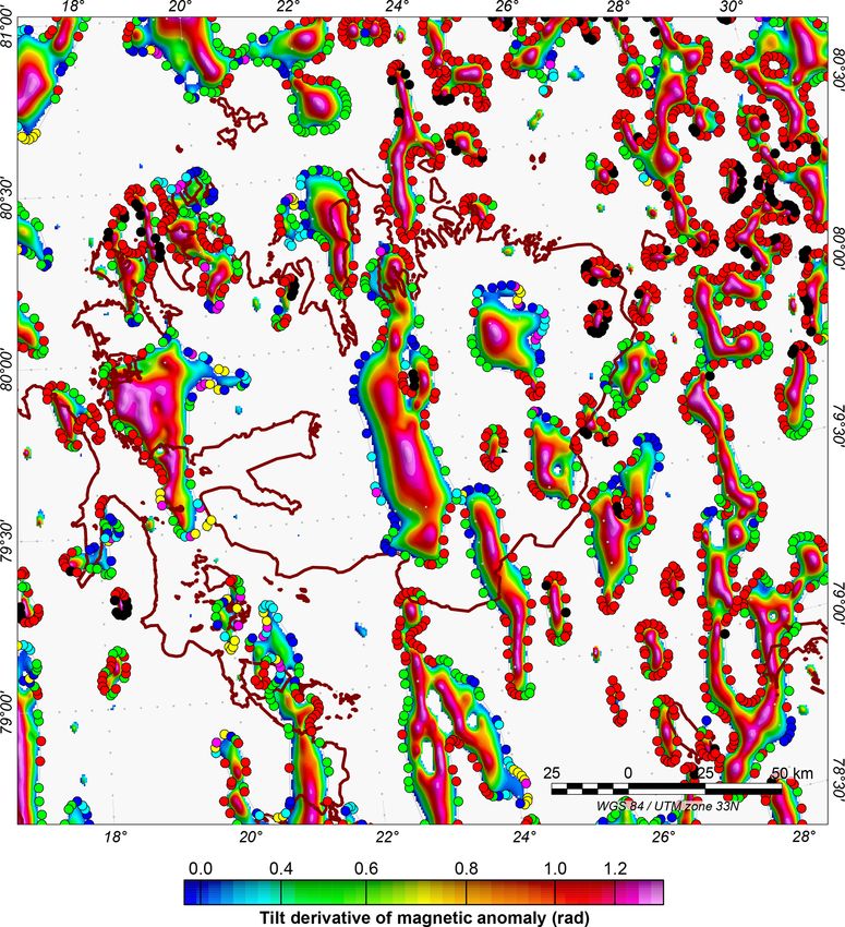
184                           M.-A. Dumais and M. Brönner: Revisiting Austfonna, Svalbard, with potential field methods

temperate ice. For temperatures at pressure melting point,
common in temperate glaciers, liquid water is present at the
ice–bed interface. The correctness of the resulting topogra-
phy depends on several glacier parameters, including density,
porosity and the water content fraction, which determine the
permittivity and, therefore, the radio wave velocity used to
derive the thickness (Lapazaran et al., 2016). These parame-
ters cannot be directly measured and are highly influenced by
temporal and spatial variations of the water content fraction
distribution through the glacier (Barrett et al., 2007; Navarro
et al., 2009; Jania et al., 2005).
   Using GPR and radio-echo sounding (RES) measurements
from several campaigns, a bed topography has been derived
for Austfonna on Svalbard (Fürst et al., 2018; Dunse et al.,
2011). In this paper, we test the feasibility of retrieving the
glacier thickness of Austfonna with airborne gravity data,
as they are sensitive to the density contrast between the ice
and the bedrock. Adding magnetic interpretation to the study
contributes by indicating variations in the bedrock lithology
and the density distribution, which must be considered to ac-
curately derive ice thickness and bedrock topography. Com-
bined gravity–magnetic interpretation is a powerful tool to
define basement types and identify the presence of various
geological structures, such as sedimentary basins under the            Figure 1. Surface topography map of Nordaustlandet, east of
ice in the bedrock. Gravity and magnetic methods have been             Spitsbergen, Svalbard, and the Austfonna icecap from Dunse et
used in the past for basement lithology studies in the Arctic          al. (2011). Approximately 80 % of Nordaustlandet is covered by ice,
                                                                       and the ice thickness is up to ca. 600 m. Polythermal and relatively
(e.g. Gernigon et al., 2018; Døssing et al., 2016; Nasuti et al.,
                                                                       flat at its highest elevation, Austfonna hosts both land-terminating
2015; Gernigon and Brönner, 2012; Olesen et al., 2010; Bar-
                                                                       and tidewater glaciers of which several have been observed to surge.
rère et al., 2009) and for sea ice and glacier studies (e.g. An
et al., 2017; Gourlet et al., 2015; Tinto et al., 2015; Zhao et
al., 2015; Porter et al., 2014; Tinto and Bell, 2011; Studinger
et al., 2008, 2006; Spector, 1966). In this study, we com-             basal sliding and subglacial water might be present. Surging,
bine these methods with GPR data to obtain both an accu-               or surge-type, glaciers have also been observed in the area
rate glacial bed topography and also an understanding of the           (Schytt, 1969). Other studies link surging to the softness of
rheological changes of the basement. Magnetic and gravity              the bedrock and tectonically active zones (e.g. Jiskoot et al.,
modelling were used to assess the feasibility of retrieving to-        2000). The bedrock topography (including cavities and ob-
pographical and geophysical properties in terms of ice thick-          stacles), geothermal sources and the presence of sediments
ness, bed softness, the presence of carbonates and till, and           are also contributing factors to the glacier basal-sliding ve-
bed topography.                                                        locities (e.g. Boulton and Hindmarsh, 1987; Clarke, 1987).
                                                                          During the last few decades, several campaigns have
                                                                       aimed to retrieve the underlying bedrock topography of Aust-
2   Austfonna and its underlying geology                               fonna using RES (Moholdt et al., 2010a; Dowdeswell et
                                                                       al., 1986) and GPR (Dowdeswell et al., 2008; Dunse et al.,
With a geographic area of 8357 km2 , Austfonna, seen in                2011). Acquired profiles are shown in Fig. 2. McMillan et
Fig. 1, is the largest icecap on the Svalbard archipelago (Dall-       al. (2014) and Moholdt et al. (2010a, b) applied satellite al-
mann, 2015). It is located on Nordaustlandet, the second-              timeter data to estimate surface elevation changes and ice
largest island in Svalbard, northeast of Spitsbergen, and ap-          loss. They observed a significant increase in the dynamic
proximately 80 % of it is covered by ice. Austfonna has one            activity and the outlet flow rate of the glaciers Vestfonna
main central dome with an ice thickness of up to 600 m                 (Schäfer et al., 2012) and Austfonna (McMillan et al., 2014).
(Dowdeswell et al., 1986) and feeds several drainage basins.           Over 28 % of the area covered by Austfonna rests below sea
Considered polythermal, consisting of a mixture of temper-             level (Dowdeswell et al., 1986). Moreover, the lowest eleva-
ate and cold ice, it is relatively flat at its highest elevation and   tions of the bedrock are located at the tips of Basin 3 in the
includes both land-terminating and tidewater glaciers. Stud-           southeast and Leighbreen in the northeast, (Fig. 1), with bed
ies suggest its basal temperature is near the pressure melt-           elevation values of 150 and 130 m below sea level, respec-
ing point (Dunse et al., 2011); thus Austfonna experiences             tively (Dunse et al., 2011; Dowdeswell et al., 2008).

The Cryosphere, 14, 183–197, 2020                                                             www.the-cryosphere.net/14/183/2020/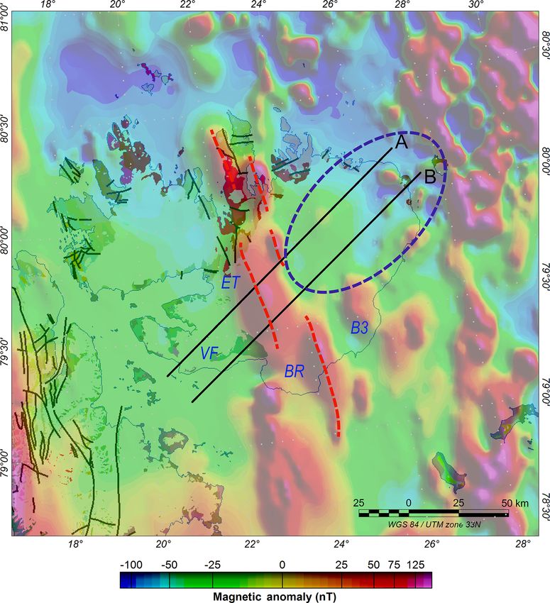
M.-A. Dumais and M. Brönner: Revisiting Austfonna, Svalbard, with potential field methods                                               185

Figure 2. Geological map of Austfonna with GPR and RES campaign lines and gravity–magnetic profiles A and B (modified from Dallmann,
2015, and Dunse et al., 2011). The interpreted profiles, labelled A and B, have been chosen to cover a large area of Austfonna and to capture
important geological trends.

   The geology underneath the ice is barely understood, as               den continues under Austfonna. The southern basement of
very few outcrops are available to identify the main geo-                Austfonna is believed to be much younger than the one
logical structures and basement affinity of Nordaustlandet               in the north and is composed of unmetamorphosed post-
(Fig. 2). However, based on the studied outcrops, the ge-                Caledonian rocks. The youngest rocks in Nordaustlandet are
ology appears to be complex and the exposed rocks are                    Jurassic–Cretaceous doleritic dikes, which intrude into the
dated to various geological epochs (Dallmann, 2015; Johans-              Tonian basement rocks (composed of dolomite, sandstone,
son et al., 2002). Basement outcrops at Wahlenbergfjorden                quartzite and limestone) on the island of Lågøya, and the
identify different types of basements on each side of the                Meso- to Neoproterozoic basement composed of basal con-
fjord (Dallmann, 2015), which is assumed to represent a                  glomerate, volcanic breccias and migmatites in the outlet of
major geological north–south (N–S) division of the island.               Brennevinsfjorden, northwest of Vestfonna (Overrein et al.,
For the northern shore of the fjord and north of Nordaust-               2015). South of Nordaustlandet, dolerite sills were emplaced
landet (including the totality of Vestfonna), the regional map           during the Cretaceous in Kong Karls Land. Evidence of the
of Lauritzen and Ohta (1984) and radiometric dating (Ohta,               locations of the sills can be found in seismic-reflection and
1992) indicate a pre-Caledonian basement with Mesopro-                   magnetic data in the vicinity of Nordaustlandet (Polteau et
terozoic and Neoproterozoic rock exposures, mainly com-                  al., 2016; Minakov et al., 2012; Grogan et al., 2000).
posed of metasedimentary rocks like marble, quartzite and
mica schist. The rocks are significantly folded and faulted
due to the Caledonian-deformation influence but not to the
                                                                         3   Magnetic and gravity data
same degree as in the rest of Svalbard. Caledonian and
Grenvillian Rijpfjorden granites are found on the northern
tip of Nordaustlandet on Prins Oscars Land (Johansson et                 The magnetic map is a compilation of two datasets compiled
al., 2005, 2002). In the east, the bedrock comprises mainly              from campaign flights flown in 1989 and 1991 (Table 1). The
Silurian diorites and gabbros as seen on Storøya (Johans-                data are sparse with line spacing of 4 to 8 km at a target
son et al., 2005). On the southern shore of Wahlenbergfjor-              ground clearance of 900 m. Having been originally processed
den, an abundance of Carboniferous to Permian limestones                 by different entities with different processing algorithms, the
and dolomites with Early Cretaceous doleritic intrusions are             datasets are reprocessed to a similar level. A control line,
exposed. Dallmann (2015) consequently concluded that the                 flown during both campaigns as an overlap, is used to level
same geological demarcation observed at Wahlenbergfjor-                  the two datasets to each other. This step ensures that the two
                                                                         datasets are levelled to the standard International Geomag-

www.the-cryosphere.net/14/183/2020/                                                                The Cryosphere, 14, 183–197, 2020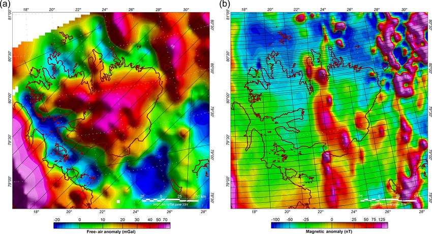
186 M.-A. Dumais and M. Brönner: Revisiting Austfonna, Svalbard, with potential field methods
netic Reference Field (IGRF) model (Thébault et al., 2015) the measurements (Fig. 2) suggests lower resolution in ar-
and the compilation is smooth at the overlap. eas with poor coverage. With these data, combined with the
The magnetic map (Fig. 3b) presents strong parallel ice surface topography published by the Norwegian Polar In-
anomalies crossing the centre of Nordaustlandet, oriented N– stitute (NPI) in 1998 (Norwegian Polar Institute, 1998), an
S. The magnetic intensity is correlated with the type and ice thickness is derived for Austfonna. This step allows for
level of magnetization, which in turn is mainly related to an estimate of the volume and mass of the icecap to derive
the iron content, time of formation or metamorphic processes the gravitational effect of the glacier. The density contrast
of the minerals found in the basement. Thus, the magnetiza- and the topography of the bedrock–ice interface contribute to
tion is a strong indicator of the mineralogy of the basement the sharpest and most prominent gravity effects. A valid ap-
and its lithology. The strong anomaly observed across Aust- proach to resolve the bedrock topography is to assume a sim-
fonna also intersects the Caledonian Rijpfjorden granites, ple basement geometry with a homogeneous density. Anal-
which have been identified on the geology map (Johansson ogous to sedimentary-basin interpretation (Bott, 1960) and
et al., 2005). This anomaly is also parallel to the Billefjorden treating the glacier as an infinite slab, the free-air anomaly
fault zone and to the Caledonian frontal thrust (Gernigon and (FAc ) along a profile is reconstructed as follows:
Brönner, 2012; Barrère et al., 2009). The Caledonian is also
associated with magmatic episodes. Northeast of Nordaust- FAc = 2π Gρice hice + 2π G (ρbed − ρice ) Hice
landet, the sharp and low-frequency magnetic anomalies cre- + 2π Gρbed hbed , (1)
ated by the known emplaced Cretaceous sills have a distinct
and prominent signature. where G is the gravitational constant (6.67 ×
The gravity data were acquired during a 1998–1999 cam- 10−11 N m2 kg−2 ), ρ the density, hbed the topography
paign (Forsberg and Olesen, 2010; Forsberg et al., 2002). The of the bed above sea level, and hice and Hice the thickness
flight routes were along a southwest–northeast (SW–NE) di- of ice above sea level and below sea level, respectively. The
rection with a spacing of 18 km and at a ground clearance full extent of the ice thickness is represented by (hice + Hice ).
of 1 km (Table 1). The free-air anomaly map is presented The free-air anomaly is referenced to the geoid. In the
in Fig. 3a. The gravity data produced 4000 m cell size grids reconstruction of the free-air anomaly, the ice above sea
with a standard deviation of ∼ 2 mGal over a 6000 m half- level is regarded as an excess of mass, whereas the ice below
wavelength resolution. Gravity lows are seen in the south and sea level is considered a mass deficiency. The influence
southwest of Nordaustlandet, with a higher signal on the ice- of the ice (ρice = 910 kg m−3 ) depends on the surrounding
cap reflecting the ice coverage and its thickness. Gravity is media, which include air (ρair ≈ 1 kg m−3 , negligible) and
sensitive to the density contrast between the various geolog- the bed (ρbed = 2670 kg m−3 ) in this case. This reduction
ical bodies and ice in this case. Low-gravity measurements technique is valid under the condition that the thickness
reflect low densities, which are often linked to sediment ac- of the ice is smaller than the horizontal dimensions of the
cumulation or sedimentary basins. icecap by several magnitudes. As GPR and RES data were
The grid resolution provides an estimate of the smooth- acquired solely onshore, only onshore gravity acquisition
ness level of the data and of the limitations to the mod- was considered in the model for comparison.
elling and data filtering. Given the magnetic grid resolu- Assuming the difference between the free-air anomaly ob-
tion, features shallower than 2 km cannot be accurately re- served (FAo ) and the free-air anomaly calculated is caused
solved. Depth interpretations and body geometry are limited by erroneous bed topography measurements, the correction
by the grid resolution. A single anomaly normally leads to of the bed topography is as follows:
several geometry and depth possibilities. In this paper, the
(FAo −FAc )
most favourable possibility is chosen for its consistency with 2πG(ρbed −ρice )
if the bed topography is below sea level
the GPR and RES investigations and for model simplicity. ∂hbed = (2)
Therefore, depth estimates from the models in the present
(FAo −FAc )
2πG(ρ )
paper represent the deepest depth possibility and are limited
bed
if the bed topography is above sea level.
by a 2 km resolution. The magnetic data also present several
asymmetric anomalies which can be interpreted by dipping On average, this correction is 2 m for the analysis along the
bodies. However, given the coarseness of the data, a simple gravity profiles above Austfonna. With a standard deviation
model without dipping is preferred. of 63 m, the difference in thickness varies between −190 and
290 m. The difference in thickness is applied to the initial
bedrock topography derived from GPR and RES. Given the
4 Bed topography revisited wide line spacing of the gravity profiles, both datasets are
gridded with the same resolution (4000 m) for the analysis
Dunse et al. (2011) have presented a bedrock topography (Fig. 4). The highest summits of the bed topography remain
compilation with a 1 km spatial grid resolution from data ac- at the same level. Small residual discrepancies are largely due
quired by RES and GPR, but the geospatial distribution of to the approximation of an infinite slab and the accuracy of
The Cryosphere, 14, 183–197, 2020 www.the-cryosphere.net/14/183/2020/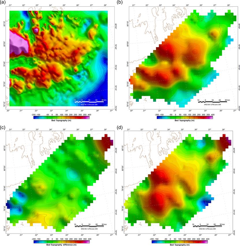
M.-A. Dumais and M. Brönner: Revisiting Austfonna, Svalbard, with potential field methods                                                 187

Table 1. Survey acquisition parameters of the magnetic and gravity compilation.

                            Compilation                              Magnetic                             Gravity
                            Line spacing                                4–8 km                         18 km
                            Aircraft altitude (approx.)                  900 m                        1000 m
                            Grid resolution                               2 km                          4 km
                            Acquisition                            1989–1991                      1998–1999
                            Acquired by                            Sevmorgeo      Norwegian Mapping Authority
                                                            Amarok and TGS             Danish Geodata Agency
                                                          University of Bergen

Figure 3. (a) Free-air gravity map and (b) a magnetic anomaly map of Nordaustlandet with the acquisition flight lines denoted by the thin
black lines. The gravity data are sensitive to an excess or loss of mass. Low free-air gravity data are often linked to sedimentary basins. The
magnetic data show important N–S-trending anomalies crossing Nordaustlandet and intersecting with the Caledonian Rijpfjorden granites.

the various datasets. It should be noted that both GPR–RES                ice surface topography increase the misfit where the glacier
depth measurements and gravity ice thickness were calcu-                  geometry is most susceptible to drastic variations. Notably,
lated with the same ice surface topography dataset which acts             the gravity profiles cross the glacier perpendicular to its flow
as a control variable. It reduces the influence of the resolution         and parallel to the shore with an uneven mass distribution;
and accuracy of the ice surface topography when compar-                   i.e. more mass is found on the northern side of the profile.
ing the two bed topography models. However, important dis-                This terrain effect is commonly corrected for in gravity pro-
crepancies exist, for example, under Vegafonna on the south-              cessing for extreme topography relief (Lafehr, 1991) but re-
west corner of Austfonna and under Leighbreen and Wors-                   quires accurate terrain topography acquired through methods
leybreen, northeast of Austfonna. These areas are discussed               such as laser scanning data acquisition or a high-resolution
in detail in later sections when magnetic data are included in            digital elevation model.
the interpretation. Less prominent misfits occur at the outer
edge of the marine-terminating glaciers Basin 3 and Bråsvell-
breen, where the ice surface topography and glacier geome-                5   2-D forward models
try might undergo rapid and drastic variations, and where rel-
atively faster ice surface velocities were observed in compar-            Interpretation using 2-D forward modelling determines the
ison to the thick, flat interior icecap (Gladstone et al., 2014;          interface between contrasting bodies of different magneti-
Moholdt et al., 2010a). As the ice surface topography and                 zations and densities. It provides depth and geometrical in-
gravity data were acquired around the same time but inde-                 sights into lithological variations in the bedrock. The forward
pendently of each other, the resolution and accuracy of the               modelling (Fig. 5) is carried out along the actual airborne
                                                                          gravity lines to ensure the highest resolution of the gravity

www.the-cryosphere.net/14/183/2020/                                                                 The Cryosphere, 14, 183–197, 2020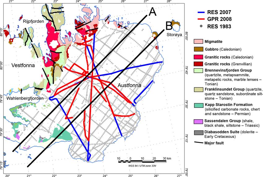
188                           M.-A. Dumais and M. Brönner: Revisiting Austfonna, Svalbard, with potential field methods

Figure 4. Bed topography derived from RES and GPR (a), bed topography derived from RES and GPR gridded along gravity acquisition
flight lines (b), corrections applied to the bed topography (c) and bed topography corrected for gravity measurements gridded along gravity
profiles (d). Major discrepancies with deviations greater than 150 m occur under Vegafonna (southwest) and Leighbreen and Worsleybreen
(northeast).

data. Two lines are modelled and referred to as profiles A              mann, 2015). The basement is forward modelled according
and B (Fig. 2). The modelled profiles were chosen for their             to gravity and magnetic signatures, using the software pack-
location and coverage. They contain several aspects of the              age GM-SYS (Geosoft, 2006). The mantle–crust boundary,
geology under Austfonna (such as basements and intrusions),             i.e. the Mohorovičić discontinuity (Moho), was set at a depth
and they are located near or above RES and GPR measure-                 of around 33 km following the interpretation of Ritzmann et
ments. Models are initially constrained by the bedrock topog-           al. (2007). In the northeast of Austfonna, the basement seems
raphy derived by Dunse et al. (2011) and are independent of             to have a very low magnetization (less than 0.001 SI), but a
the free-air bed topography corrections. The measured data              density higher than the surrounding media (2700 kg m−3 ) is
points from the GPR and RES are highlighted (purple cir-                required to fit the observed field.
cles, Fig. 5a).                                                            Along profile A (Fig. 5a), reducing the density in the
   Initial petrophysical parameters are assigned based on the           southwest of Austfonna (where Vegafonna is located) was at-
comprehensive petrophysical database from mainland Nor-                 tempted but could not be fit to the observed free-air anomaly.
way (Olesen et al., 2010) provided by the Geological Survey             Introducing layers of till with a density of 1600 kg m−3 did
of Norway (NGU) and on the described bedrock types (Dall-               not significantly reduce the signal to account for the observed

The Cryosphere, 14, 183–197, 2020                                                              www.the-cryosphere.net/14/183/2020/
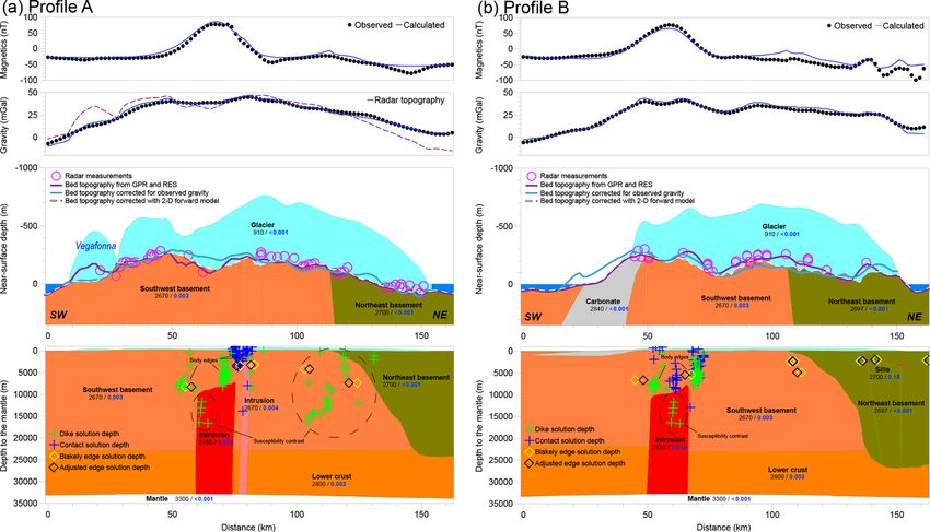
M.-A. Dumais and M. Brönner: Revisiting Austfonna, Svalbard, with potential field methods                                               189

Figure 5. Observed and calculated magnetic and gravity profiles (top), the near-surface view of the basements (middle) and the depth to
the mantle (bottom) for profile A (a) and profile B (b), as defined in Fig. 2, with Werner deconvolution indicators of the intrusions and the
basement interfaces. A gravity response (purple solid lines) is calculated for a homogeneous bedrock using GPR–RES bed topography. The
misfit with the observed gravity measurements suggests the bedrock is heterogeneous and the bed topography from the radar needs refining.
The gravity-corrected bed topography (blue lines in the near-surface view panel) is an improvement but fails to recognize the heterogeneity
of the bed. The 2-D forward model (dashed white line) improves the accuracy of the bed topography by using a density more representative
of the lithology. Each section representing a geological body is characterized with a density (kg m−3 ; black values) and a susceptibility
(SI units; blue values). Dike solution depths (green crosses), contact solution depths (blue crosses), Blakely edge solution depths (yellow
diamonds) and adjusted-edge solution depths (black diamonds) are identified.

gravity data unless the till had a thickness of several hundreds         D forward model than predicted from the gravity correction.
of metres. Thus, the GPR–RES bed topography is adjusted in               The 2-D forward model accounts both for a certain degree of
this area to be consistent with the gravity measurements. This           confidence in the GPR–RES data and for the bedrock density
discrepancy is more important under a region with scarce                 variation.
GPR and RES measurements (measurements are indicated                        The centres of both profiles are characterized by a
with purple circles). A similar interpretation was made along            high magnetic anomaly requiring high susceptibility. This
profile B, where misfits between the two methods occur and               anomaly is a prominent and continuous N–S-oriented
only a few measurements exist. The GPR–RES data were not                 anomaly, which might at least be partly linked to exposed
acquired in a grid pattern, and therefore the GPR–RES bed                granites on Prins Oscars Land at the northern tip of Nor-
topography proposed in these discrepancy areas is the result             daustlandet. A relatively high density of 2725–2750 kg m−3
of a gridding interpolation between profiles and data points.            is assigned to this granitic intrusion. However, granites
The bed topographies calculated from the free-air analysis               with comparable densities and susceptibilities are found
and interpreted from magnetic and gravity modelling agree                on the mainland of Norway in Vest-Agder, Rogaland and
in general and suggest corrections to the GPR–RES topogra-               Telemark (NGU petrophysics database available at http://
phy in the same direction. However, misfits exist, since the             geo.ngu.no/GeosciencePortal/, last access: 29 March 2019;
free-air analysis presented in the previous section considers            2016). Werner deconvolution (Phillips, 1997; Ku and Sharp,
a homogenous basement, while the model interpretation in-                1983; Werner, 1955), an automated depth-to-source estima-
dicates variable densities. The difference between the GPR–              tion method, was applied to help quantify the depth and mor-
RES bed topography and the 2-D forward-model bed topog-                  phology of magnetic bodies under Austfonna (Fig. 5a and b).
raphy varies from −170 to 80 m with a standard deviation                 Using these empirical basement indicators that are sensitive
of 40 m. A smaller level of correction is required with the 2-           to susceptibility variations, and approximating the geological

www.the-cryosphere.net/14/183/2020/                                                                The Cryosphere, 14, 183–197, 2020
190 M.-A. Dumais and M. Brönner: Revisiting Austfonna, Svalbard, with potential field methods
source to a simplified geometry of features such as contacts
and dikes (Goussev and Peirce, 2010), the depth and edges of
intrusions were estimated. Euler deconvolution (Thompson,
1982; Reid et al., 1990), with a structural index of 1 (for dike
and sill models), was also used to compare the results. This
method uses horizontal and vertical derivatives along with a
predetermined structural index to estimate the source loca-
tion. In our case, Euler deconvolution analyses provide sim-
ilar depth values to those from Werner deconvolution anal-
yses. Both Werner and Euler deconvolution analyses deter-
mined the existence of a dike at a depth of about 8 km with
a width of almost 20 km. While Euler deconvolution results
in a dike seated at 8 km, Werner deconvolution resolves the
top of this intrusion to be tilted with a depth from 8 km in
the southwest to 6 km in the northeast. A second dike was
determined at a 2 km depth (or 1.5 km with Euler deconvo-
lution) with a much narrower width of 2 km and was only
seen on profile A, indicating a dike also shorter in length.
The model suggests shallow magnetized bodies exist off the
shore of Nordaustlandet with a depth of less than 2 km. These
indications are used in the model to constrain the depth of the
intrusions. Given the accuracy of the data, a certain degree of
freedom is allocated to those indicators to fit the observed
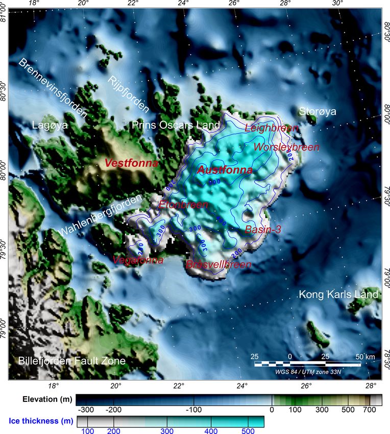
Figure 6. The tilt derivative of the magnetic anomaly superimposed
data with the geology expected.
by Blakely depth estimation is used to determine the location and
The gridded tilt derivative of an anomaly, at a location x, y depth of geological bodies and to constrain the model. Negative data
(Miller and Singh, 1994), characterizes the angle of the ratio are nulled. Sill bodies located in northeast Austfonna, both onshore
between the amplitudes of the vertical derivative and the hor- and offshore, are generally shallower than the large and deep N–S-
izontal derivative. Thus, the zero contour indicates the border trending granitic intrusions crossing Austfonna.
of a geological body where a density or susceptibility con-
trast with the surrounding media occurs. This indication from
the magnetic tilt derivative (Fig. 6) was used to constrain the a common magnetization value for sills of 0.15 SI suscep-
lateral extent of the intrusions. Blakely et al. (2016) have also tibility (Hunt et al., 1995). Another major difference be-
developed a method to retrieve the edge of a body and its tween the two profiles modelled is the higher-density body
depth (Fig. 5) by using the reciprocal of the horizontal gradi- (2840 kg m−3 ) located west of the intrusions on profile B.
ent at the zero contour of the tilt derivative grid (Fairhead et The NPI geological map identifies a carbonate outcrop in
al., 2008; Salem et al., 2007). At high magnetic latitudes for this area of Austfonna. This carbonate body has a strong in-
a vertical dike geometry, the depth is estimated as equal to fluence on the gravity signal, which is critical in the estima-
the half-width of the magnetic anomaly (Hinze et al., 2013). tion of the bed topography (turquoise topography, Fig. 5b).
The lateral edge of the body is adjusted accordingly to the Locally, the bed has a much higher density and should be
depth found with Blakely’s method (2016). This reduces the considered when making bed topography corrections. The
size of the magnetic body (Fig. 5) to the minimum size re- magnetic and gravity modelling provides an indication of this
quired for this depth. Thus, a first magnetic body with a sus- carbonate depth, orientation and thickness. Given the coarse-
ceptibility 0.004 SI in a 0.003 SI surrounding, a density of ness of the data and their limitations, the carbonate body is
2670 kg m−3 , a width of 3 km and a depth of 2 km is mod- expected to be shallower and thinner.
elled. The top of the second intrusion is deeper (10 km) and
wider (15 km) with higher magnetic and density properties
(0.016 SI and 2750 kg m−3 ). For both profiles, the difference 6 Bed lithology revisited
between the bed topography from the magnetic–gravity in-
The results from the 2-D modelling of profiles A and B are
terpretation and the gravity estimation is caused by the large
summarized in Fig. 7. According to the models, a promi-
density intrusion located in the basement.
nent deep-seated, highly magnetic intrusion occurs under-
Along profile B, anomalies of smaller sizes are found on
neath Austfonna crossing N–S, and the bedrock is divided
the eastern coastline of Austfonna. The nature of the mag-
into two types of basement with different geophysical prop-
netic signal and the results from Euler and Werner decon-
erties.
volutions suggest the existence of shallow magmatic bodies
such as sills. For simplification, they were modelled with
The Cryosphere, 14, 183–197, 2020 www.the-cryosphere.net/14/183/2020/M.-A. Dumais and M. Brönner: Revisiting Austfonna, Svalbard, with potential field methods 191
ties suggested by the susceptibility and density interpreted in
the 2-D forward models, the high magnetic anomalies cor-
respond to the geological mapping of the observed granites
(Fig. 7). Therefore, granite intrusions are proposed to exist in
Nordaustlandet bedrock, such as the Caledonian Rijpfjorden
granites seen on the central northern tip of Nordaustlandet
(Johansson et al., 2005). These intrusions, trending N–S to
NNW–SSE like the major faults found on Prins Oscars Land,
suggest the faults are present and continue under Austfonna.
Along profile B, sill intrusions are modelled on the east-
ern coastline, where shallow sills have been previously inter-
preted and related to a tholeiitic phase (130–100 Ma) linked
to the spreading of the Amerasia Basin in the Arctic Ocean
and the uplift initiated by the mantle plume on the Yermak
Plateau, northwest of Svalbard (Polteau et al., 2016; Minakov
et al., 2012; Grogan et al., 2000).
Densities found under southwest Austfonna are also lower
compared to the northeastern region. This is consistent with
the terrain observations under the Etonbreen and Bråsvell-
breen basins (Dunse et al., 2015, 2011), suggesting a more
erodible bedrock in the southwestern area. It correlates
with the late Paleozoic platform composed of limestones,
dolomites, carbonate rocks and sedimentary rocks to the
Figure 7. Profiles A and B, as defined in Fig. 2, against the mag-
southwest of Austfonna compared to the metasedimentary
netic anomaly and NPI geological map. Dashed red lines represent
deep intrusion trends across Austfonna and the blue circle repre-
rocks (marble, quartzite and mica schist) from the pre-
sents the change of basement seen on the lines modelled (B3: Basin Caledonian basement found to the northeast. Furthermore,
3; ET: Etonbreen; BR: Bråsvellbreen; VF: Vegafonna). the 2-D model suggests a smoother bed topography than the
one suggested by GPR–RES measurements, which is con-
sistent with a more erodible basement. While two types of
bedrock are already expected from outcrop samples, the anal-
Given the densities and susceptibilities used and the pres- ysis of the two profiles suggests an oblique division (NE–
ence of granites on the northern part of the island, the intru- SW) between the two basement types rather than a N–S divi-
sion is likely to be granitic. It is probably of a different com- sion. The younger basement is more constrained to the north-
position than the exposed rocks, since the modelled granitic east of Austfonna than previously thought. An oblique divi-
densities indicate relatively high values but are within the sion of the basement is consistent with the major fault sys-
expected values for granites (2500–2810 kg m−3 ; Telford et tem found on Svalbard and the geological provinces division
al., 1990). Moreover, given the N–S-trending faults system (often separated by faults), both trending N–S to NNW–SSE
across Svalbard, a similar process could explain the strong (Harland et al., 1974; Flood et al., 1969).
magnetic anomalies trending N–S and crossing Nordaust-
landet. Major faults on Svalbard, trending N–S to north-
northwest–south-southeast (NNW–SSE), have been reacti- 7 Methodology assessment
vated and juxtaposed by strike-slip motion over several ge-
ological periods before, during and after the Caledonian Additional magnetic and gravity data improve the bed accu-
orogeny (Dallmann, 2015). Granites were emplaced during racy and the spatial resolution by filling gaps in the GPR–
the late stages of the Caledonian (late Silurian to Early Devo- RES data. Austfonna bed topography was assessed and re-
nian) (Dallmann, 2015). One could argue the presence of N– calculated using free-air anomaly measurements. The bed
S-striking sills in the near-offshore region could correspond topography was enhanced and refined using the 2-D model
to the magnetic signature seen under Austfonna. However, interpretation, and its physical properties were extracted.
the frequency content of the magnetic signal (derived from Given the scarce sampling of the GPR–RES data under Ve-
high-frequency filters or vertical derivatives), the size of the gafonna, the discrepancies might be due to gridding interpo-
structures revealed from tilt derivative signals and the depth lation (Fig. 3), as previously discussed. Similarly, along pro-
estimates from Werner deconvolution suggest the existence file B, the poorer fit of the bed topography derived from GPR
of a rather wide (15 km), deep-seated (10 km) dike intrusion and RES with the magnetic and gravity model is caused by
or dike complex onshore and shallow bodies offshore and on the scarcer availability of GPR–RES data. Another source of
the coastline of Austfonna. In addition to the granite affini- error is the accumulation of water in the erodible basement,
www.the-cryosphere.net/14/183/2020/ The Cryosphere, 14, 183–197, 2020192 M.-A. Dumais and M. Brönner: Revisiting Austfonna, Svalbard, with potential field methods
causing an increase in uncertainty and underestimation of the
ice thickness. The magnetic and gravity data provide con-
sistent and regular coverage over the full area and are less
sensitive to gridding interpolation. Gravity data processing
requires the use of high-precision GPS measurements, which
were estimated to have a 0.5 m vertical accuracy (Forsberg et
al., 2002). In comparison, the distribution of GPR and RES
measurements shows irregularities mainly due to the poor
navigational guidance available at the time of acquisition
(Dowdeswell et al., 1986; GlaThiDa Consortium, 2019). The
navigational errors caused flight-line distortions and wider
line spacings in certain areas. Positional errors were esti-
mated as ±250 m (Dowdeswell et al., 1986). Therefore, the
GPR–RES bed topography is more prone to gridding inter-
polation artefacts. GPR–RES measurements are susceptible
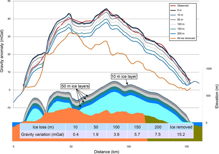
to thickness errors in the presence of steep bed slopes, where Figure 8. Predicted gravity signature variations with ice loss. The
the signal is reflected from a lateral wall instead of the bot- gravity response is calculated using, as the initial state, the 2-D
tom topography. While often corrected with a 2-D migra- forward model from profile A with the currently known ice thick-
ness. Uniform layers of ice with thicknesses of 10, 50, 100, 150 and
tion processing technique that corrects for the direction of
200 m are removed from the model. The first 10 m layer of ice loss
profiling, transversal slopes are not corrected unless 3-D mi- yields a gravity anomaly of approximately 0.5 mGal. Significant ice
gration is used (Lapazaran et al., 2016; Moran et al., 2000). loss is detectable from long-term observations.
The water content in the glacier and the bedrock increases in-
ternal scattering and the dielectric absorption. It also affects
the radio wave velocity, which contributes to the error in the
time-to-thickness conversion (Brown et al., 2017; Lapazaran tion of ∼ 2 mGal over a 6000 m half-wavelength resolution.
et al., 2016; Blindow et al., 2012; Matsuoka, 2011). Tem- Bed topography corrections with gravity data are more effec-
poral and spatial variations of radio wave velocity account tive than GPR–RES gridding interpolation algorithms. The
for uncertainties in ice thickness reconstruction (Jania et al., spatial resolution of airborne gravity measurements depends
2005; Navarro et al., 2014). The magnetic and gravity inter- on the gravimeter together with the platform stability, line
pretation compensates indirectly for these errors, as it is less spacing, acquisition speed and distance to the source. A state-
sensitive to water content in the bedrock and offers an addi- of-the-art fixed-wing airborne gravimeter, flown with the ap-
tional control on the properties of the bedrock. The magnetic propriate flight parameters, can produce 200 m cell size grids
data show the bedrock heterogeneity, associated with sus- with a precision of ∼ 0.5 mGal over a 3000–4000 m half-
ceptibility variations within the glacier bed, indicating differ- wavelength resolution (e.g. An et al., 2019, 2017; Studinger
ent bedrock types and lithologies. These lithological changes et al., 2008). Therefore, using gravity modelling increases
suggest the presence of geological boundaries and provide the confidence in and the accuracy of the bedrock topography
constraints to assigning density changes. Thus, the magnetic under a glaciated area. Improvement of the spatial resolution
data improve the final bed topography accuracy, as they pro- of the final bed topography could also be achieved with the
vide constraints on the density distribution for the bed under- appropriate survey parameters and a denser line spacing for
lying the glacier. The effect of geology on gravity inversion the gravity data.
for glacial bed topography was also noticed in other studies Till, commonly found at the base of the glacier, can ac-
(An et al., 2019, 2017; Hodgson et al., 2019). count for the misfit between the observed and modelled grav-
Using Austfonna bed topography and lithology derived ity but could not be resolved given the resolution of the
from the 2-D forward model, the theoretical gravity response dataset. For a variation of 1 mGal, 50 m of till (1600 kg m−3 )
was modelled for ice loss by removing iteratively uniform needs to be emplaced in the model. Lower flight elevation
and homogeneous layers of ice (Fig. 8). The model predicts and denser line spacing acquisition is required to model the
that an ice thickness variation of 10 m causes an average vari- till. For the accurate interpretation of till modelling, addi-
ation in gravity of ∼ 0.5 mGal, which is resolved by state- tional independent measurements are required, such as mag-
of-the-art gravity measurements. Thus, the gravity anomaly netic data which are sensitive to the susceptibility contrast
is mainly driven by the bedrock topography and its physical with the surrounding bedrock.
properties, providing hard evidence of the interface between Due to their chemical composition, calcium carbonate
the ice and the rock. The cell size of the GPR–RES-gridded rocks erode subglacially and migrate in the glacier system
bed topography is 1000 m with extensive interpolation be- along various transportation paths (Bukowska-Jania, 2007).
tween the measurements. Flown in 1998–1999, the gravity Calcite dissolution and precipitation have an impact on the
data produced 4000 m cell size grids with a standard devia- calcite saturation of the water film that lubricates the bed–
The Cryosphere, 14, 183–197, 2020 www.the-cryosphere.net/14/183/2020/M.-A. Dumais and M. Brönner: Revisiting Austfonna, Svalbard, with potential field methods 193
glacier interface, and they modify the bed morphology and alyzing them can lead to a better understanding of the sliding
roughness through melting and regelation processes (Ng and mechanisms in the area.
Hallet, 2002). The model from profile B suggests carbonate
rocks underlie the glacier, and it maps the lateral extent of the
body by an additional 7–8 km under the ice. While the thick- 8 Conclusions
ness of the carbonate is small compared to the resolution of
the data, the gravity measurements suggest an important ex- Airborne magnetic and gravity data were used to study the
cess of mass at that location but with no susceptibility varia- Austfonna icefield basement on Svalbard. Considering a ho-
tion from the surrounding media. Therefore, we must expect mogenous basement, the GPR–RES bed topography was cor-
there to be a prominent volume of carbonate with an assumed rected with gravity measurements. We demonstrated the im-
density of 2840 kg m−3 . portance of the geology for a gravity inversion to calculate
Deep intrusions, possibly granites, and shallow sills were the bed topography and presented a method that integrates
located and delineated from the 2-D forward model. Char- magnetic, gravity, GPR and RES data. Several interpretation
acterization of these intrusions provides information about techniques (Euler deconvolution, Werner deconvolution, 2-D
the potential variation of the bed lithology in terms of ther- modelling) were used to create a model of the bedrock with
mal conductivity. Geothermal heat flux, resulting from the assigned physical properties in terms of size, depth, suscep-
decay of radioactive isotopes present in the glacier bed, may tibility and density. These results suggest the bed topography
raise the temperature of the basal ice and affect the ice slid- derived from GPR–RES measurements can be corrected with
ing (Paterson and Clarke, 1978). Granites are prone to higher gravity analysis, while knowledge of the basement lithology
geothermal heat flux due to their mineral composition. On and/or magnetic interpretation further increases its reliabil-
Austfonna, only one borehole has been drilled to reach the ity. Thus, the bed topography model derived from magnetic
bedrock and provide heat flux information in the summit and gravity measurements contributes to a more accurate es-
area, indicating a geothermal heat flux of ∼ 40 mW m−2 (Ig- timation of ice volume. One of the main challenges is that the
natieva and Macheret, 1991; Zagorodnov et al., 1989). There data were acquired in different campaigns, in different years
are no other direct observations available to estimate this heat and with different acquisition patterns. On the other hand,
flux. However, our study suggests that this measurement may this approach expands the coverage of the model. Given the
not be representative for the entire bed underlying Austfonna. difficulty of accessing the underlying lithology of Austfonna,
Located outside the 2-D modelled profiles, a high- increasing the magnetic and gravity coverage is an effective
intensity anomaly is apparent under Basin 3, subject to a high method to assess the physical properties of the basement.
negative ice surface elevation change rate (Gladstone et al., Moreover, the geophysical interpretation provides insight
2014; Moholdt et al., 2010a). Due to the large variation of the into the geological and structural affinity of the basement un-
ice surface topography in recent years (and decades), retriev- der Austfonna. While the presence of two basement types
ing a valid ice topography for the gravity model has proven on Nordaustlandet is well accepted, the new interpretation
difficult. However, the results from profiles A and B with allows the boundary between the basements to be mapped.
the Euler deconvolution, Werner deconvolution and Blakely The physical properties of the basements provide indications
depth methods indicate a basement that resembles the softer of the basement types for softness and erodibility and pro-
southwestern basement, largely intruded with shallow (less vide information about the type of intrusions likely found un-
than 2 km) sills and deeper (8 km) granitic intrusions. Such der the icefield. Sills, granitic intrusions and carbonate rocks
physical properties are possible drivers for the high basal- have been interpreted in the model and their evolution was set
sliding rate and surge mechanisms and can be linked to the in a geotectonic time frame. Each of these geological bod-
high ice surface elevation changes seen on Basin 3. Further ies has a different impact on the basal thermal regime and
studies of the granitic intrusion and thermal modelling would the erodibility of the basement, consequently leading to het-
be of great interest to link the geothermal flux under Basin 3 erogenous basal-ice-sliding rates.
to ice changes currently observed. The temperature of the ice at the base, which controls the
The interpretation of the two profiles provides an insight basal thermal regime, is usually determined by ice thickness,
into the basement and intrusion geology and a refined glacial ice advection, ice surface temperature, geothermal heat and
bed topography, specifically where GPR and RES data are frictional heat (related to softness and topography). Irregu-
scarce and less reliable. These findings enhance the under- lar basal topography leads to complex localized patterns of
standing of the regional geology of the area and demonstrate the thermal regime. The lithology identified with potentially
the potential to reconstruct the full bed lithology with the aid higher radiogenic heat production can be correlated with ar-
of high-resolution gravity and magnetic data. Granitic intru- eas of faster ice surface velocities or ice thickness variations.
sions are known to be potential geothermal sources and can Here, with additional petrophysical properties from collected
locally affect the heat flux profile of Austfonna. These intru- rock samples, thermal modelling is necessary and will help
sions can be linked to the basal sliding of Austfonna, and an- to improve understanding of the different geothermal do-
mains and their effects on Austfonna basal thermal regimes.
www.the-cryosphere.net/14/183/2020/ The Cryosphere, 14, 183–197, 2020194 M.-A. Dumais and M. Brönner: Revisiting Austfonna, Svalbard, with potential field methods
In this paper, the resolution of the datasets limits the reso- Bamber, J. L., Ferraccioli, F., Joughin, I., Shepherd, T., Rippin, D.
lution of the geometry of the geological features modelled. M., Siegert, M. J., and Vaughan, D. G.: East Antarctic ice stream
Higher-resolution data from state-of-the-art instrumentation, tributary underlain by major sedimentary basin, Geology, 34, 33,
i.e. gravimeters, GPS units, GPR, RES devices and magne- https://doi.org/10.1130/g22160.1, 2006.
tometers, would further refine the physical properties of the Barrère, C., Ebbing, J., and Gernigon, L.: Offshore prolongation of
Caledonian structures and basement characterisation in the west-
basement and allow for a full reconstruction of the bed lithol-
ern Barents Sea from geophysical modelling, Tectonophysics,
ogy and topography. 470, 71–88, https://doi.org/10.1016/j.tecto.2008.07.012, 2009.
Barrett, B. E., Murray, T., and Clark, R.: Errors in radar CMP ve-
locity estimates due to survey geometry, and their implication
Data availability. Bed elevation data are available from Dunse et for ice water content estimation, J. Environ. Eng. Geophys., 12,
al. (2011). Magnetic and revised bed topography data are available 101–111, https://doi.org/10.2113/jeeg12.1.101 2007.
on the Geological Survey of Norway Geoscience Portal (http://geo. Blakely, R. J., Connard, G. G., and Curto, J. B.: Tilt Derivative
ngu.no/GeosciencePortal/search, last access: 21 November 2019; Made Easy, Geosoft Technical Publications, 4, 1–4, 2016.
Geological Survey of Norway Geoscience Portal, 2016; contact per- Blindow, N., Salat, C., and Casassa, G.: Airborne GPR sounding
son is Marie-Andrée Dumais). Gravity data are available upon re- of deep temperate glaciers – Examples from the Northern Patag-
quest from the Norwegian Mapping Authority (contact person is onian Icefield, 2012 14th International Conference on Ground
Ove Omang) or on the Geological Survey of Norway Geoscience Penetrating Radar (GPR), 664–669, 2012.
Portal. Bott, M. H. P.: The use of rapid digital computing methods for
direct gravity interpretation of sedimentary basins, Geophys.
J. Royal Astro. Soc., 3, 63–67, https://doi.org/10.1111/j.1365-
Author contributions. MAD reprocessed the airborne magnetic 246x.1960.tb00065.x, 1960.
dataset and produced the bed topography from the gravity data and Boulton, G. S. and Hindmarsh, R. C. A.: Sediment de-
the 2-D forward model. MB assisted in the data interpretation and formation beneath glaciers: rheology and geologi-
commented on the paper. cal consequences, J. Geophys. Res., 92, 9059-9082,
https://doi.org/10.1029/JB092iB09p09059, 1987.
Brown, J., Harper, J., and Humphrey, N.: Liquid water content in ice
Competing interests. The authors declare that they have no conflict estimated through a full-depth ground radar profile and borehole
of interest. measurements in western Greenland, The Cryosphere, 11, 669–
679, https://doi.org/10.5194/tc-11-669-2017, 2017.
Bukowska-Jania, E.: The role of glacier system in migration of cal-
Acknowledgements. We would like to thank Thorben Dunse for cium carbonate on Svalbard, Pol. Polar Res., 28, 137–155, 2007.
providing the GPR–RES bed and related surface elevation maps and Clarke, G. K. C.: Subglacial till: A physical framework for its
for his helpful discussions on the data. We thank Rene Forsberg and properties and processes, J. Geophys. Res., 92, 9023–9036,
Ove Omang for providing the airborne gravity data. Chantel Nixon https://doi.org/10.1029/jb092ib09p09023 1987.
is also acknowledged for English proofreading of an earlier version Clarke, G. K. C.: Subglacial Processes, Ann.
of the paper. We thank Daniel Farinotti and the three anonymous re- Rev. Earth Planet. Sci., 33, 247–276,
viewers for their valuable comments that improved the manuscript. https://doi.org/10.1146/annurev.earth.33.092203.122621, 2005.
Dallmann, W. K.: Geoscience Atlas of Svalbard, Norsk polarinsti-
tutt Rapportserie, 2015.
Døssing, A., Jaspen, P., Watts, A. B., Nielsen, T., Jokat, W., Thybo,
Review statement. This paper was edited by Daniel Farinotti and
H., and Dahl-Jensen, T.: Miocene uplift of the NE Greenland
reviewed by three anonymous referees.
margin linked to plate tectonics: Seismic evidence from the
Greenland Fracture Zone, NE Atlantic, Tectonics, 35, 1–26,
https://doi.org/10.1002/2015tc004079, 2016.
Dowdeswell, J., Drewry, D., Cooper, A., Gorman, M., Liestøl, O.,
References and Prheim, O.: Digital mapping of the Nordaustlandet ice caps
from airborne geophysical investigations, Ann. Glaciol., 8, 51–
An, L., Rignot, E., Elieff, S., Morlighem, M., Millan, R., Moug- 58, https://doi.org/10.1017/s0260305500001130, 1986.
inot, J., Holland, D. M., Holland, D., and Paden, J.: Bed eleva- Dowdeswell, J. A., Hagen, J. O., Björnsson, H., Glazovsky,
tion of Jakobshavn Isbrae, West Greenland, from high-resolution A. F., Harrison, W. D., Holmlund, P., Jania, J., Ko-
airborne gravity and other data, Geophys. Res. Lett., 44, 3728– erner, R. M., Lefauconnier, B., Ommanney, C. S. L., and
3736, https://doi.org/10.1002/2017gl073245, 2017. Thomas, R. H.: The Mass Balance of Circum-Arctic Glaciers
An, L., Rignot, E., Millan, R., Tinto, K., and Willis, J.: Bathymetry and Recent Climate Change, Quaternary Res., 48, 1–14,
of Northwest Greenland Using “Ocean Melting Greenland” https://doi.org/10.1006/qres.1997.1900, 1997.
(OMG) High-Resolution Airborne Gravity and Other Data, Re- Dowdeswell, J. A., Benham, T. J., Strozzi, T., and Hagen, J. O.:
mote Sens., 11, 131, https://doi.org/10.3390/rs11020131, 2019. Iceberg calving flux and mass balance of the Austfonna ice cap
Bahr, D. B., Pfeffer, W. T., and Kaser, G.: A review of on Nordaustlandet, Svalbard, J. Geophys. Res., 113, F03022,
volume-area scaling of glaciers, Rev. Geophys., 53, 95–140, https://doi.org/10.1029/2007JF000905, 2008.
https://doi.org/10.1002/2014RG000470, 2015.
The Cryosphere, 14, 183–197, 2020 www.the-cryosphere.net/14/183/2020/M.-A. Dumais and M. Brönner: Revisiting Austfonna, Svalbard, with potential field methods 195
Dunse, T., Greve, R., Schuler, T. V., and Hagen, J. O.: Permanent Cryosphere, 8, 1393–1405, https://doi.org/10.5194/tc-8-1393-
fast flow versus cyclic surge behavior: numerical simulations 2014, 2014.
of the Austfonna ice cap, Svalbard, J. Glaciol., 57, 247–259, GlaThiDa Consortium: Glacier Thickness Database 3.0.1,
https://doi.org/10.3189/002214311796405979, 2011. World Glacier Monitoring Service, Zurich, Switzerland,
Dunse, T., Schuler, T. V., Hagen, J. O., and Reijmer, C. H.: Seasonal https://doi.org/10.5904/wgms-glathida-2019-03, 2019.
speed-up of two outlet glaciers of Austfonna, Svalbard, inferred Gong, Y., Zwinger, T., Åström, J., Altena, B., Schellenberger, T.,
from continuous GPS measurements, The Cryosphere, 6, 453– Gladstone, R., and Moore, J. C.: Simulating the roles of crevasse
466, https://doi.org/10.5194/tc-6-453-2012, 2012. routing of surface water and basal friction on the surge evolution
Dunse, T., Schellenberger, T., Hagen, J. O., Kääb, A., Schuler, of Basin 3, Austfonna ice cap, The Cryosphere, 12, 1563–1577,
T. V., and Reijmer, C. H.: Glacier-surge mechanisms promoted https://doi.org/10.5194/tc-12-1563-2018, 2018.
by a hydro-thermodynamic feedback to summer melt, The Gourlet, P., Rignot, E., Rivera, A., and Casassa, G.: Ice thickness
Cryosphere, 9, 197–215, https://doi.org/10.5194/tc-9-197-2015, of the northern half of the Patagonia Icefields of South Amer-
2015. ica from high-resolution airborne gravity surveys, Geophys.
Eyles, N., Boyce, J. I., and Putkinen, N.: Neoglacial (< 3000 years) Res. Lett., 43, 241–249, https://doi.org/10.1002/2015GL066728,
till and flutes at Saskatchewan Glacier, Canadian Rocky Moun- 2015.
tains, formed by subglacial deformation of a soft bed, Sedimen- Goussev, S. A. and Peirce, J. W.: Magnetic basement: gravity-
tology, 62, 182–203, https://doi.org/10.1111/sed.12145, 2015. guided magnetic source depth analysis and interpretation,
Fairhead, J. D., Salem, A., Williams, S., and Samson, E.: Mag- Geophys. Prosp., 58, 321–334, https://doi.org/10.1111/j.1365-
netic interpretation made easy: The Tilt-Depth-Dip- 1K method, 2478.2009.00817.x, 2010.
SEG Technical Program Expanded Abstracts 2008, 779–783, Gray, L., Burgess, D., Copland, L., Demuth, M. N., Dunse, T., Lan-
https://doi.org/10.1190/1.3063761, 2008. gley, K., and Schuler, T. V.: CryoSat-2 delivers monthly and
Flood, B., Gee, D. G., Hjelle, A., Siggerud, T., and Winsnes, T. inter-annual surface elevation change for Arctic ice caps, The
S.: The Geology of Nordaustlandet, northern and central parts, Cryosphere, 9, 1895–1913, https://doi.org/10.5194/tc-9-1895-
Norsk Polarinstitutt Skrifter, 146, 1969. 2015, 2015.
Forsberg, R. and Olesen, A. V.: Airborne Gravity Field Determi- Grinsted, A.: An estimate of global glacier volume, The
nation, in: Sciences of Geodesy – I: Advances and Future Di- Cryosphere, 7, 141–151, https://doi.org/10.5194/tc-7-141-2013,
rections, edited by: Xu, G., Springer Berlin Heidelberg, Berlin, 2013.
Heidelberg, 83–104, 2010. Grogan, P., Nyberg, K., Fotland, B., Myklebust, R., Dahlgren, S.,
Forsberg, R., Olesen, A. V., Keller, K., and Møller, M.: Airborne and Riis, F.: Cretaceous Magmatism South and East of Sval-
gravity survey of sea areas around Greenland and Svalbard 1999– bard: Evidence from Seismic Reflection and Magnetic Data, Po-
2001, Survey and processing report – KMS Technical Report, 18, larforschung, 68, 25–34, 2000.
2002. Harland, W. B., Cutbill, J. L., Friend, P. F., Gobbett, D. J., Holliday,
Fürst, J. J., Navarro, F., Gillet-Chaulet, F., Huss, M., Moholdt, D. W., Maton, P. I., Parker, J. R., and Wallis, R. H.: The Billefjor-
G., Fettweis, X., Lang, C., Seehaus, T., Ai, S., Benham, T. J., den fault zone, Spitsbergen: the long history of a major tectonic
Benn, D. I., Björnsson, H., Dowdeswell, J. A., Grabiec, M., lineament, Norsk Polarinstitutt Skrifter, 161, 1974.
Kohler, J., Lavrentiev, I., Lindbäck, K., Melvold, K., Pettersson, Hinze, W., Von Frese, R., and Saad, A.: Gravity and magnetic ex-
R., Rippin, D., Saintenoy, A., Sánchez-Gámez, Schuler, T. V., ploration: Principles, practices and applications, Cambridge Uni-
Sevestre, H., Vasilenko, E., and Braun, M. H.: The Ice-Free To- versity Press, 2013.
pography of Svalbard, Geophys. Res. Lett., 45, 11760–711769, Hodgson, D. A., Jordan, T. A., De Rydt, J., Fretwell, P. T., Seddon,
https://doi.org/10.1029/2018GL079734, 2018. S. A., Becker, D., Hogan, K. A., Smith, A. M., and Vaughan, D.
Geological Survey of Norway Geoscience Portal, available at: G.: Past and future dynamics of the Brunt Ice Shelf from seabed
http://geo.ngu.no/GeosciencePortal/search (last access: Novem- bathymetry and ice shelf geometry, The Cryosphere, 13, 545–
ber 2019), 2016. 556, https://doi.org/10.5194/tc-13-545-2019, 2019.
Geosoft: GM-SYS profile modeling. Gravity and Magnetic Model- Hunt, C. P., Moskowitz, B. M., and Banerjee, S. K.: Rock physics
ing Software, v. 4.10, Geosoft Incorporated, p. 116, 2006. and phase relations, A Handbook of Physical Constants: AGU
Gernigon, L. and Brönner, M.: Late Palaeozoic architecture and Reference Shelf, Americain Geophysical Union Vol. 3, 189–204,
evolution of the southwestern Barents Sea: insights from a 1995.
new generation of aeromagnetic data, Journal of the Geological Ignatieva, I. Y. and Macheret, Y. Y.: Evolution of Nordaustlandet
Society, London, 169, 449–459, https://doi.org/10.1144/0016- ice caps in Svalbard under climate warming, Glaciers-Ocean-
76492011-131, 2012. Aonosphere Interactions, Proceedings of the International Sym-
Gernigon, L., Brönner, M., Dumais, M.-A., Gradmann, S., posium held at St Petersburg, September 1990, IAHS Publ. no.
Grønlie, A., Nasuti, A., and Roberts, D.: Basement inher- 208, 208, 301–312, 1991.
itance and salt structures in the SE Barents Sea: Insights Iverson, N. R., Hooyer, T. S., Fischer, U. H., Cohen, D., Moore,
from new potential field data, J. Geodynam., 119, 82–106, P. L., Jackson, M., Lappegard, G., and Kohler, J.: Soft-bed
https://doi.org/10.1016/j.jog.2018.03.008, 2018. experiments beneath Engabreen, Norway:regelation infiltration,
Gladstone, R., Schäfer, M., Zwinger, T., Gong, Y., Strozzi, T., Mot- basal slip and bed deformation, J. Glaciol., 53, 323–340,
tram, R., Boberg, F., and Moore, J. C.: Importance of basal pro- https://doi.org/10.3189/002214307783258431, 2007.
cesses in simulations of a surging Svalbard outlet glacier, The Jania, J., Macheret, Y. Y., Navarro, F. J., Glazovsky, A. F.,
Valisenko, E. V., Lapazaran, J. J., Glowacki, P., Migala, K., Balut,
www.the-cryosphere.net/14/183/2020/ The Cryosphere, 14, 183–197, 2020You can also read