Road Traffic Air Quality Management - Appendices - Department of ...
←
→
Page content transcription
If your browser does not render page correctly, please read the page content below
Appendices

Road Traffic Air Quality Management
June 2014
Copyright

http://creativecommons.org/licenses/by/3.0/au/

© State of Queensland (Department of Transport and Main Roads) 2014

Feedback: Please send your feedback regarding this document to: mr.techdocs@tmr.qld.gov.au

Road Traffic Air Quality Management, Transport and Main Roads, June 2014
Amendment Register

 Issue /      Reference
                                 Description of revision            Authorised by       Date
 Rev no.       section
1                                                                                   June 2014

Road Traffic Air Quality Management, Transport and Main Roads, June 2014                        i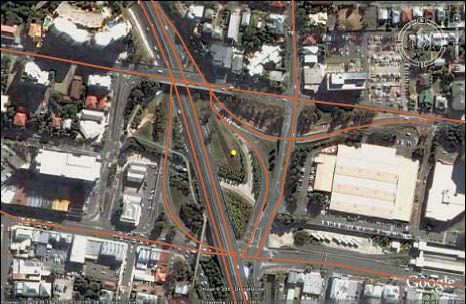
Contents

Appendix A – Modelling Example .........................................................................................................5
1      Example 1 – Road emissions .......................................................................................................5
1.1    Emissions........................................................................................................................................ 5
1.2    CALINE4 line source dispersion model .......................................................................................... 6
2      Example 2 - Construction emissions .........................................................................................10
2.1    Input parameters ........................................................................................................................... 11
2.2    Pollutants modelled ...................................................................................................................... 12
2.3    Emission factors used ................................................................................................................... 12
2.4    Source estimates .......................................................................................................................... 13
2.5    Dispersion modelling .................................................................................................................... 14
Appendix B – Tunnels ..........................................................................................................................17
1      Tunnels .........................................................................................................................................17
2      Internal air quality guidelines .....................................................................................................17
3      Parameters relevant to emission rates ......................................................................................17
3.1    Gradient ........................................................................................................................................ 17
3.2    Speed ............................................................................................................................................ 17
3.3    Emissions estimation .................................................................................................................... 17
3.4    Dispersion modelling .................................................................................................................... 18
Appendix C – Climate Change Impact Assessment .........................................................................20
1      Assessment – GHG emissions and mitigation measures .......................................................20
2      Assessment – Climate change risks and adaptation measures .............................................20
3      Calculation methods ...................................................................................................................20
Appendix D – Assessment of Potential Air Quality Impacts of Busway Projects .........................21
1      Objectives .....................................................................................................................................21
1.1    Document overview ...................................................................................................................... 21
2      Assessment philosophy .............................................................................................................22
3      Air pollutants of concern ............................................................................................................23
3.1    General ......................................................................................................................................... 23
3.2    Pollutants of interest to the Department of Transport and Main Roads ....................................... 24
4      Transport emission factors ........................................................................................................25
4.1    South-east Queensland bus fleet ................................................................................................. 25
       4.1.1     Background ..................................................................................................................25
       4.1.2     Options .........................................................................................................................26
4.2    Urban vehicle fleet ........................................................................................................................ 29
       4.2.1     Background ..................................................................................................................29
       4.2.2     Options .........................................................................................................................30
5      Air Quality Design standards .....................................................................................................31
5.1    Ambient Air Quality ....................................................................................................................... 31

Road Traffic Air Quality Management, Transport and Main Roads, June 2014                                                                                  ii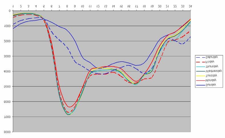
5.2 In-tunnel air quality ....................................................................................................................... 32
6 Existing air quality .......................................................................................................................33
6.1 Ambient air monitoring .................................................................................................................. 33
6.1.1 When is monitoring necessary? ...................................................................................33
6.1.2 How much monitoring is required? ...............................................................................34
6.1.3 What methods should be used for monitoring? ............................................................34
6.2 Characterisation of background levels ......................................................................................... 35
7 Project information requirements ..............................................................................................36
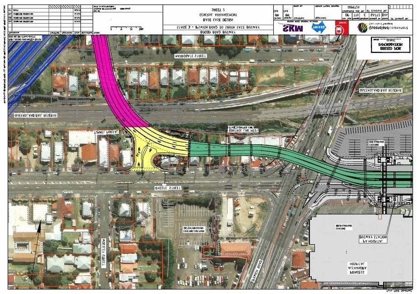
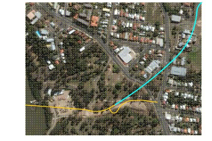
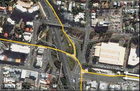
7.1 Alignment information ................................................................................................................... 36
7.1.1 Busway and road alignments .......................................................................................36
7.1.2 Gradients ......................................................................................................................38
7.1.3 Intersections .................................................................................................................38
7.1.4 Signalling information ...................................................................................................38
7.1.5 Acceleration of buses away from intersections and/or traffic lights .............................38
7.2 Tunnels ......................................................................................................................................... 39
7.2.1 Alignment and gradients ...............................................................................................39
7.2.2 Tunnel length and ventilation options ...........................................................................39
7.3 Traffic information ......................................................................................................................... 39
7.3.1 Bus volumes .................................................................................................................39
7.3.2 General vehicle traffic volumes ....................................................................................40
7.3.3 Traffic speeds ...............................................................................................................40
7.4 Fleet information ........................................................................................................................... 41
7.4.1 Fleet composition .........................................................................................................41
7.4.2 Fleet emissions inventory .............................................................................................42
8 Assessment tools and their application ....................................................................................47
8.1 Dispersion models ........................................................................................................................ 47
8.1.1 CALINE4 .......................................................................................................................47
8.1.2 CAL3QHCR ..................................................................................................................48
8.1.3 AusRoads .....................................................................................................................48
8.1.4 Ausplume ......................................................................................................................48
8.1.5 CALPUFF .....................................................................................................................48
8.1.6 TAPM ............................................................................................................................49
8.2 Meteorological models .................................................................................................................. 49
8.2.1 CALMET .......................................................................................................................49
8.2.2 TAPM ............................................................................................................................49
8.3 CFD models .................................................................................................................................. 49
8.3.1 Fluent ............................................................................................................................49
8.3.2 ARIA .............................................................................................................................49
8.4 Busway calculator ......................................................................................................................... 50
8.4.1 Overview of the BMSDC ..............................................................................................50
9 Assessment methodology ..........................................................................................................51
9.1 Level 1 and Level 2 assessments................................................................................................. 51
9.2 Level 1 assessment ...................................................................................................................... 52
9.2.1 When to implement?.....................................................................................................52
9.2.2 Emission inventory .......................................................................................................52
9.2.3 Assessment tools .........................................................................................................52
9.2.4 Methodology .................................................................................................................53
9.3 Level 2 assessment ...................................................................................................................... 53
9.3.1 When to implement?.....................................................................................................53
9.3.2 Emission inventory .......................................................................................................54
Road Traffic Air Quality Management, Transport and Main Roads, June 2014 iii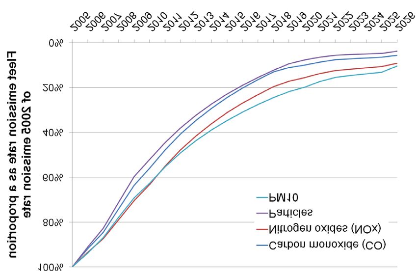
9.3.3           Meteorological data ......................................................................................................54
       9.3.4           Assessment tools .........................................................................................................55
       9.3.5           Methodology .................................................................................................................55
10     Reporting and results presentation ...........................................................................................55
10.1 Pollutant species ........................................................................................................................... 55
     10.1.1     Nitrogen dioxide............................................................................................................56
     10.1.2     Carbon monoxide .........................................................................................................56
     10.1.3     Particulate matter .........................................................................................................56
     10.1.4     Ultrafine particles ..........................................................................................................56
     10.1.5     Volatile organic compounds .........................................................................................57
10.2 Scaling versus modelling .............................................................................................................. 57
10.3 Presentation of results at sensitive receptor locations ................................................................. 58
     10.3.1     Tables ...........................................................................................................................58
     10.3.2     Time series ...................................................................................................................58
     10.3.3     Hour of day ...................................................................................................................58
     10.3.4     Ground-level concentrations a function of wind direction.............................................59
10.4 Contour plots of the study area..................................................................................................... 60
10.5 Study limitations ............................................................................................................................ 60
11     Suggestions for further work .....................................................................................................60
11.1 Gaps in knowledge ....................................................................................................................... 60
11.2 Extension of knowledge ................................................................................................................ 61
12     Additional details .........................................................................................................................61
12.1 Defining linkages .......................................................................................................................... 61
12.2 Links: free flowing buses .............................................................................................................. 61
12.3 Links: tunnel portals ...................................................................................................................... 62
12.4 Links: idling buses at bus stations and intersections .................................................................... 62
12.5 Summary of busway links ............................................................................................................. 63
12.6 Assigning gradients ...................................................................................................................... 64
12.7 Receptor grid ................................................................................................................................ 64
12.8 Hourly bus load profile .................................................................................................................. 64
12.9 Other modelling parameters ......................................................................................................... 64
13     References ....................................................................................................................................66

Road Traffic Air Quality Management, Transport and Main Roads, June 2014                                                                             iv
Appendix A: Modelling Examples

Appendix A – Modelling Example

1           Example 1 – Road emissions
This example shows how to calculate air pollutant emissions for a section of road using the Transport
and Main Roads Excel spreadsheet tool MRD_emfac_scenario.xls and then calculate the ambient
concentration of pollutants using the CALINE4 dispersion model.

This example considers a new road of four lanes, modelled as three links. On each row of the Table 1
below, the coordinates of one end of each road segmented are tabulated, together with the Annual
Average Daily Traffic (AADT), speed limit and percentage heavy vehicles for the link ending at that
point. Thus the three values on the last three columns of the first line of data will be ignored.

Table1: Road and traffic input information for modelled scenario

                                                            AADT            Speed limit         Heavy
            x (m)         y (m)           z (m)
                                                          (veh/day)           (km/h)          Vehicles (%)
              0             0               0
            1000          1000             50               10000                 60                10
            2000          1000             120              5000                  80                5
            3000          2000             130              5000                  80                5
The layout of the road and receptors in the example is shown in Figure 1.

Figure 1: Road example layout - plan view, showing receptor locations

                                  Road and Receptors

            2000

            1500
    y (m)

            1000

             500

                  0
                      0   500      1000           1500      2000           2500        3000
                                                 x (m)

1.1          Emissions

Emissions for a section of road comprising several segments are calculated using the Transport and
Main Roads Excel spreadsheet tool MRD_emfac_scenario.xls.

Road Traffic Air Quality Management, Transport and Main Roads, June 2014                                 5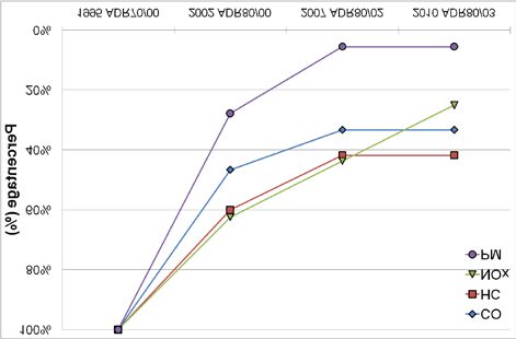
Appendix A: Modelling Examples

When the spreadsheet is opened, a grid input area is visible in which the above data can be typed.
Data can then be saved as an input scenario for future reference by clicking on the button labelled
Save input file and then specifying a file name and location.

The spreadsheet has been set up to calculate emission rates for pollutants as g/vehicle/km or
g/vehicle/mile. The g/vehicle/mile unit is required for input to CALINE4. Clicking on the Checkbox
labelled Output emissions per mile selects the appropriate unit.

Clicking on the button labelled Save output file calculates emissions for each link and stores them in
an Excel Comma Separated Variable (CSV) file which can be opened in Excel to display the results.
An example of such output (formatted slightly) appears in Table 2 below.

Table 2: Calculated vehicle emissions using spreadsheet tool

                          NOx         CO           HC           PM10           SO2       Fuel        CO2e
      Conditions         g/veh/      g/veh/       g/veh/       g/veh/         g/veh/    L/veh/      kg/veh/
                          mile        mile         mile         mile           mile      mile        mile
AADT = 10 000
Speed = 60              6.66        30.54        1.84        0.25             0.22      0.26        0.65
Heavy_Veh = 10
Speed = 80
                        7.12        33.78        1.71        0.28             0.26      0.33        0.81
AADT = 5000
Heavy_Veh = 5           4.58        28.14        1.36        0.16             0.17      0.19        0.46
                                                                                                    CO2e
                        NOx g/s     CO g/s       HC g/s      PM10 g/s         SO2 g/s   Fuel L/s
Totals                                                                                              kg/s
                        1473.2      7268.8       413.8       54.2             50.1      62.4        154.1
The emissions spreadsheet tool can also input a road from a file containing a single road centreline
string in Autocad DXF format, provided that the centreline is defined as a continuous set of line
segments or a single polyline (an Autocad entity that defines a set of end-to-end line segments).

1.2      CALINE4 line source dispersion model

The CALINE4 model is freely available from the Internet. It models a road as a number of straight
segments, each associated with a constant air pollutant emission rate in units of g/vehicle/mile. It also
requires data on traffic volumes and meteorological conditions.

CALINE4 is a DOS style program that requires a fairly rigid input format and is not very user-friendly.
A Windows style front end program called CL4 can be downloaded with CALINE4. After installation, it
can be used to produce input files for CALINE4 and to run the program.

CL4 is somewhat limited in that it only allows a limited range of inputs – for example, only allowing
calculation of the concentration of carbon monoxide (CO).

However, the input file produced by CL4 can be edited manually using a program such as WordPad to
calculate concentrations of other pollutants.

Alternatively, the concentration of pollutants other than CO can be calculated by scaling the output in
CO ppm units produced for the emission rate of the other pollutant by a density scale factor
(28 g/mol x 1000 L/m3 / 22.4 L/mol = 1250 g/m3) that converts ppm of CO to µg/m3.

For example, if an emission rate of 10 g/vehicle/mile of CO produces 3.1 ppm of CO, then
2 g/vehicle/mile of NOx (reported as NO2) will result in a concentration of
2 / 10 x 3.1 x 1250 = 775 µg/m3 of NOx.

Road Traffic Air Quality Management, Transport and Main Roads, June 2014                                    6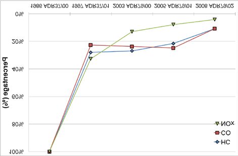
Appendix A: Modelling Examples

For the data generated by the spreadsheet for Summer of 2005, CALINE4 was set up as follows:

    •   3 links – A, B and C

    •   Hourly traffic volume 1000 vehicles/hour

    •   Pollutant - CO (only pollutant calculated by CL4)

    •   Wind direction – worst angle

    •   Wind speed – low wind, worst case recommended by USEPA

    •   Stability - Stability Class G (worst case, highly stable, low dispersion)

    •   Mixing height 500m (not critical for receptors near road unless very low, rarely low when traffic
        volumes are high)

    •   Surface roughness 100 cm (suburban)

    •   Sigma theta 10 degrees

    •   Temperature 15 degrees C

    •   Receptors at 20, 40, 60, 80, 100 and 150 metres from the road centreline, height 1.8 m

    •   No ambient background CO

The output was as follows:

    •   CALINE4: CALIFORNIA LINE SOURCE DISPERSION MODEL

    •   JUNE 1989 VERSION

    •   PAGE 1

    •   JOB: Transport and Main Roads Ex 1

    •   RUN: Hour 1 (WORST CASE ANGLE)

    •   POLLUTANT: Carbon Monoxide

I. SITE VARIABLES

U= 1.0 M/S                           Z0= 100. CM                           ALT= 0. (M)
BRG=WORST CASE                       VD= .0 CM/S
CLAS= 7 (G)                          VS= .0 CM/S
MIXH= 500 M                          AM B= .0 PPM
SIGTH= 10. DEGREES                   TEMP= 15.0 DEGREE (C)

II. LINK VARIABLES

    LINK                                                                        EF            H     W
                               LINK COORDINATES                  TYPE
 DESCRIPTION                                                                VPH (G/MI)    (M)       (M)
A. Link A             0          0         1000       1000       AG         1000 28.2    .0       20.0
B. Link B             1000       1000      2000       1000       AG         1000 33.8    .0       20.0
C. Link C             2000       1000      3000       2000       AG         1000 28.1    .0       20.0

Road Traffic Air Quality Management, Transport and Main Roads, June 2014                                  7
Appendix A: Modelling Examples
III. RECEPTOR LOCATIONS
RECEPTOR COORDINATES (M)
1. Recpt 1 1500 1020 1.8
2. Recpt 2 1500 1040 1.8
3. Recpt 3 1500 1060 1.8
4. Recpt 4 1500 1080 1.8
5. Recpt 5 1500 1100 1.8
6. Recpt 6 1500 1150 1.8
CALINE4: CALIFORNIA LINE SOURCE DISPERSION MODEL
JUNE 1989 VERSION
PAGE 2
OB: Transport and Main Roads Ex 1
RUN: Hour 1 (WORST CASE ANGLE)
POLLUTANT: Carbon Monoxide
IV. MODEL RESULTS (WORST CASE WIND ANGLE )
PRED CONC / LINK (PPM)
BRG
RECEPT CONC
DEG A B C
PPM
1. Recpt 1 259. 1.9 .2 1.6 .0
2. Recpt 2 254. 1.2 .3 1.0 .0
3. Recpt 3 253. 1.0 .3 .8 .0
4. Recpt 4 250. .9 .3 .3 .0
5. Recpt 5 248 .9 .3 .5 .0
6. Recpt 6 243. .8 .4 .4 .0
The direction of wind is reported as the direction from which the wind blows toward the road, ranging
from 0° (north), clockwise through 90° (east), 180° (south) and so on. It can be seen from the results
above that the worst case wind direction for receptor 1, which is 20 m from the centre of the road, is
259° or 11° south of west. This produces a maximum concentration of 1.9 ppm, with 0.2 ppm coming
from Link A and 1.6 ppm from Link B. As the distance from the road increases, the worst case wind
angle swings further to the south and the concentration drops to 0.8 ppm at a distance of 150 m.
Because there is no way to change the format of the output, the accuracy of displayed results is
limited. To produce a more precise output, it is possible to increase the input emission rates by a
factor of say 50 or 100, and then divide the results by the same factor as shown below.
Road Traffic Air Quality Management, Transport and Main Roads, June 2014 8Appendix A: Modelling Examples
IV. MODEL RESULTS (WORST CASE WIND ANGLE)
PRED CONC/LINK (PPM)
BRG
RECEPT CONC
DEG A B C
PPM
1. Recpt 1 259. 1.864 .250 1.614 .0
2. Recpt 2 254. 1.236 .274 0.962 .0
3. Recpt 3 253. 1.032 .280 .752 .0
4. Recpt 4 250. .924 .302 .622 .0
5. Recpt 5 248. .860 .316 .546 .0
6. Recpt 6 243. .778 .350 .426 .0
A plot of the results showing the variation of worst case hourly CO concentration with distance from
the road is provided in Figure 2.
Figure 2: Plot of predicted concentration vs distance from road centreline
2.00
1.75
CO concentration (ppm)
1.50
1.25
1.00
0.75
0.50
0.25
0.00
0 20 40 60 80 100 120 140
distance (m)
As previously stated, the worst hourly concentration of NOx can be calculated by multiplying the
predicted concentration of CO by the ratio of emissions of NOx compared to CO and by the conversion
factor 1250. In this case, the predicted concentration of NOx reported as NO2 at 20 m is
1.864 x 7.12 / 33.78 x 1250 = 491.1 µg/m3 of NOx.
Chapter 4 of the Air Quality Manual notes the finding of Cox et al (2005) that 10% of NOx is in the form
of NO2 at distances to 20 m. Hence the maximum hourly NO2 concentration at 20 m should be
491.1 x 10% = 49 µg/m3.
For freeways, the NO2/NOx ratio is assumed to increase linearly to 30% at 60 m for the evening peak
periods. However, the predicted concentration of CO has dropped from 1.864 ppm at 20 m to
1.032 ppm at 60 m, and the corresponding NOx concentration from 491.1 µg/m3 to 271.9 µg/m3.
Hence the worst case hourly concentration of NO2 at 60 m is predicted to be 81.6 µg/m3. It can be
seen from Table 3 that the highest concentration of NO2 may occur at a significant distance from the
road.
Road Traffic Air Quality Management, Transport and Main Roads, June 2014 9Appendix A: Modelling Examples
Table 3: Calculation of nitrogen dioxide concentrations using Cox (2005) freeway conversion
factors
NOx as NO2 Conversion
Distance (m) CO (ppm) NO2 (µg/m3)
(µg/m3) Factor
20 1.864 491.1 10% 49.1
40 1.236 325.6 20% 65.1
60 1.032 271.9 30% 81.6
80 0.924 243.4 65% 158.2
100 0.86 226.6 100% 226.6
150 0.778 205.0 100% 205.0
This worst case analysis assumes that the worst case meteorological conditions occur at the same
time as the worst case traffic and the highest NO2 conversion rates. If predicted concentrations are
significant in relationship to recommended air quality guidelines, a more detailed analysis of the
occurrence of worst case wind speed, direction and stability parameters is warranted.
Chapter 4 of the Air Quality Manual notes the findings of a central Brisbane study that for periods of
8 hours, 24 hours, 90 days and 12 months, the maximum concentrations can be obtained from peak
one hour concentrations by using multiplicative concentration ratios (persistence factors) of 0.4, 0.24,
0.14 and 0.06 respectively. Table 4 shows results for other averaging times using these procedures as
well as the guideline values.
Table 4: Pollutant concentrations calculated using EPA Brisbane persistence factors and
guideline levels
Distance (m) CO (ppm) 8 hr NO2 (µg/m3) 1 hr PM10 24 hr SO2 24 hr
20 0.75 49.1 4.6 4.3
40 0.49 65.1 3.1 2.9
60 0.41 81.6 2.6 2.4
80 0.37 158.2 2.3 2.1
100 0.34 226.6 2.1 2.0
150 0.31 205.0 1.9 1.8
Guideline 9 246 50 100
If pollutant concentrations are significant in relation to guideline levels, it would be preferable to
undertake modelling of each hour of the year to compile statistics for the relevant averaging times.
If air pollutant concentrations (including a 90th percentile background) for a new road are predicted to
exceed 80% of guidelines at sensitive locations within 10 years of construction, control or design
measures should be adopted with the aim of reducing pollutant levels below 80% of guidelines as
discussed in Chapter 3 of the manual.
2 Example 2 - Construction emissions
In this example, emissions from a road construction activity are calculated using emission factors from
the NPI and EPA AP-42 handbooks. These emissions are then input, together with meteorological
data derived from the TAPM model, into the Ausplume dispersion model to calculate dust
concentrations and deposition rates.
Road Traffic Air Quality Management, Transport and Main Roads, June 2014 10Appendix A: Modelling Examples
• Activities modelled
• Emissions are assumed to arise from the following activities:
• Soil/subsoil excavation and loading to haul trucks
• Spoil transport by truck on unpaved haul roads
• Spoil dumping
• Dozer ripping and pushing activities
• Grading
• Movement of trucks carrying gravel
• Dumping of gravel
• Movement of light vehicles on unpaved roads
• Wind-blown dust from unpaved areas
• Wind-blown dust from stockpile loading/unloading
Scenarios such as this will typically be constructed to model emissions at the peak of activities, or
when activities are close to some sensitive location.
2.1 Input parameters
The parameters assumed are as follows:
Road length 500 m
Road width 25 m
Depth excavated 2m
Soil/subsoil density 2.12 t/m3
Haul truck capacity 50 t
Haul truck gross mass 55 t
Haul distance round trip 1.5 km
Days hauling 60 days
Silt 1 content 5%
Road moisture content 0.5%
Average wind speed 3 m/s
Small vehicle trips 100 per day
Average s.v. trip length 0.5 km
Average s.v. speed 60 kph
Bulldozing activity 10 h/day
Grading activity 10 h/day
1 Silt comprises particles smaller than 75 micrometers (µm) in diameter in the road surface materials. The silt
fraction is determined by measuring the proportion of loose dry surface dust that passes a 200-mesh screen,
using the ASTM-C-136 method.
Road Traffic Air Quality Management, Transport and Main Roads, June 2014 11Appendix A: Modelling Examples
Grading speed 11.4 km/h
Open area 2.5 ha
Gravel deliveries 100 t/day
Gravel truck capacity 20 t
Proportion to stockpile 50%
2.2 Pollutants modelled
This example considers only particulate emissions in the form of TSP and PM10. Emission factors are
also available for gaseous pollutants from various types of equipment for example, Table 4 of the NPI
Emission Estimation Technique Manual for Mining, but these are not considered in this example as
they are modelled in the same manner.
2.3 Emission factors used
The emission factors used in this example scenario are summarised in Table 5 and Table 6 for TSP
and PM10 respectively.
Table 5: Emission factor estimates for TSP
Assumed control
Source Emission Factor Equation Units
efficiency
Loading spoil 0.74 * 0.0016 * (U/2.2)1.3 * (M/2)-1.4 kg/t -
Hauling spoil 2.82 * (S/12)A * (W/3)B / (M/0.2)C kg/VKT 75%
Dumping spoil 0.012 kg/t 70%
(6*(S/12)1*(KPH/1.6/30)0.3 /
Small vehicle movements g/VKT 75%
(M/0.5)0.3-0.00047)*281.9
Bulldozing 2.6*S1.2*M-1.3 kg/h -
Grading 0.0034*S2.5 kg/VKT -
Gravel dumping to
0.004 kg/t 50%
stockpile
Loading from stockpile 0.03 kg/t 50%
Open area wind 0.4 kg/ha/h 75%
U = mean wind speed (m/s)
M = Moisture content in %
S = silt content in %
W = vehicle gross mass in tonnes
A = 0.8
B = 0.5
C = 0.4
VKT = vehicle kilometres travelled
KPH = vehicle speed in kph
Road Traffic Air Quality Management, Transport and Main Roads, June 2014 12Appendix A: Modelling Examples
Table 6: Emission factor estimates for PM10
Assumed control
Source Emission Factor Equation Units
efficiency
Loading spoil 0.74 * 0.0016 * (U/2.2)1.3 * (M/2)-1.4 kg/t -
Hauling spoil 2.82 * (S/12)A * (W/3)B / (M/0.2)C kg/VKT 75%
Dumping spoil 0.012 kg/t 70%
(6*(S/12)1*(KPH/1.6/30)0.3 /
Small vehicle movements g/VKT 75%
(M/0.5)0.3-0.00047)*281.9
Bulldozing 2.6*S1.2*M-1.3 kg/h -
Grading 0.0034*S2.5 kg/VKT -
Gravel loading to stockpile 0.004 kg/t 50%
Loading from stockpile 0.03 kg/t 50%
Open area wind 0.4 kg/ha/h 75%
Abbreviations as below Table 5, except:
B = 0.4
C = 0.3
References: Small vehicle movements AP42 Ch 13.2.2-4 (11/06) Eq 1b and Table 13.2.2-2
Other sources: Emission Estimation Technique Manual for Mining Version 2.3, 5 December 2001
2.4 Source estimates
The above emission factor data and equations are typically entered into an Excel spreadsheet and
calculated emissions are converted into units of g/s (for point sources) or g/m 2/s (for area sources).
Summaries of the above for the various activities and sources are provided in Table 7 and Table 8.
Road Traffic Air Quality Management, Transport and Main Roads, June 2014 13Appendix A: Modelling Examples
Table 7: Estimated emission rates for various activities
Assigned TSP PM10
Activity
source (g/s) (g/s)
Loading spoil 1 0.126 0.0597
Hauling spoil 3 0.184 0.0478
Dumping spoil 5 0.0368 0.0132
Small vehicle movements 3 0.109 0.0342
Bulldozing 1, 4, 5 2.08 0.440
Grading 1, 4, 5 0.251 0.112
Gravel hauling 3 0.0347 0.00902
Gravel dumping 4 0.00417 0.00149
Gravel loading to stockpile 2 0.00116 0.000492
Gravel loading from stockpile 2 0.0347 0.00376
Open area wind 2 0.0458 0.0229
Table 8: Estimated emission rates for various sources
Source area TSP TSP PM10 PM10
Source
(m2) (g/s) (g/m2/s) (g/s) (g/m2/s)
1 1 250 0.903 7.215E-041 0.244 1.950E-04
2 2 500 0.0209 8.380E-06 0.00901 3.924E-06
3 12 500 0.362 2.899E-05 0.108 8.670E-06
4 1 250 0.780 6.238E-04 0.186 1.484E-04
5 1 250 0.812 6.499E-04 0.197 1.578E-04
Note 1: Number format notation 7.215E-04 is equivalent to 7.215 x 10⁻⁴ or 0.0007215
In this example of a long, straight road, the number of sources is small and the geometry is simple. In
real life, more sources with more complex geometry and emission behaviour may need to be
considered.
If annual averages are being calculated for a long term project and activities move with time, the
results of the modelling of several scenarios may need to be combined.
In the example, emissions have been assumed constant over all hours. If winds have a diurnal
variation or if some sources operate at particular times, an hourly emission profile could be used to
provide more accurate predictions.
2.5 Dispersion modelling
Programs such as Ausplume, TAPM, Calpuff, Aermod and ISCST can be used to model dispersion
from roads. Models such as TAPM and Calpuff are designed to model dispersion from large industrial
sources, are probably over-complex and have insufficient resolution of dust dispersion near
construction sites. Given the likely accuracy of the emissions data, simple, fast-running models such
as Ausplume and ISCST are considered more appropriate. In this example, Ausplume is used to
calculate concentrations of dust from the above sources.
Road Traffic Air Quality Management, Transport and Main Roads, June 2014 14Appendix A: Modelling Examples When running Ausplume, it is usually best to select the menu item Edit and then the menu item Sequential Inputs. This will prompt the user to enter all the appropriate data in sequence and select appropriate input options through a series of input forms. A context-sensitive help file is accessible from each form to explain the meaning of the various options presented. A suitable meteorological file for any particular location can generally be constructed from measured wind and solar radiation data obtained at the site. If limited site-specific information is available, a file such as that used in this example can be constructed. However, it should be validated where possible against measured wind speed and direction measurements and adjusted where necessary if systematic differences are noted. Frequency analysis of several years of data can demonstrate that a particular year's data chosen for modelling is representative of typical long-term conditions. For this example, a meteorological input file was constructed for each hour of year using the TAPM meteorological model with synoptic data for 2005 and local terrain data for Brisbane. Terrain does not generally affect dust dispersion from surface sources greatly as the air in the surface layer tends to follow the terrain contours at a fairly constant height. During stable conditions, there is some tendency for vertical air motions to be suppressed and for the wind to flow around obstacles, but most standard models do not handle such situations well. However, emissions during such conditions are generally low because they tend to occur at night when dew is present, wind speeds are low and dust-generating equipment is not operating. The averaging times relevant to dust concentration are generally annual for TSP and 24 hour and annual for PM10. For dust deposition, the long term average TSP deposition rate is required. Three month and/or annual averages would be appropriate. Table 11-9.1 of AP42 Chapter 11.9 (Final Section, Supplement E, October 1998) provides estimates of the proportions of particles in the size ranges less than 30, 15, 10 and 2.5 µm in diameter. Representative diameters in these size ranges can be used in the dry depletion section to model dust fallout if site-specific information is not available. Output from the model will be in the form of a report of predicted levels at discrete locations or a contour plot of predicted levels over a region. Ausplume interfaces directly with the Surfer graphical package and so can present high-quality graphical representations of the predicted impact of emissions from the project. To enable use of Surfer, calculations are made over a suitably spaced grid of receptor points. Surfer interpolates contour lines representing equal concentrations or deposition rates over the area modelled. Interface of Ausplume with Surfer is managed automatically by Ausplume, although the user can adjust titles, axes labels, background images and so on. A contour plot of modelled emissions for sources with one year of constant emissions and no depletion appears below. Road Traffic Air Quality Management, Transport and Main Roads, June 2014 15
Appendix A: Modelling Examples

Figure 3: Ausplume plot of TSP annual average concentration
                    500

                    400

                    300

                    200

                    100
Northing (metres)

                      0

                    -100

                    -200

                    -300

                    -400

                    -500
                           -300   -200   -100   0      100    200     300     400    500   600   700   800
                                                TSP concentration (µg/m³) annual average

More realistic modelling would result from the inclusion of depletion due to fallout, attention to the
effects of source height and the use of a variable source input file that would allow for different
emissions for each hour of the year from each source.

Modelling of dust dispersion is a difficult subject, with emissions expected to vary markedly with
meteorological and operational conditions (wind, watering, revegetation, re-entrainment, particle
capture, mechanical breakdown of soil particles, vehicle operations etc). Hence modelling will normally
be indicative only of those areas on which control and monitoring activities will need to focus. A
detailed and comprehensive environmental management plan incorporating monitoring and
appropriate control strategies will be of prime importance to maintain environmental values in the
surrounding area and minimise the likelihood of nuisance or health impacts.

Road Traffic Air Quality Management, Transport and Main Roads, June 2014                                     16
Appendix B: Tunnels Appendix B – Tunnels 1 Tunnels Covered roadways in excess of 90 m in length should be considered as tunnels. Details about various aspects of tunnel design can be found in Chapter 23 of Transport and Main Roads' Road Planning and Design Manual (RPDM). This Manual covers aspects of air pollution relating to the emission of pollutants emitted from vehicle exhausts, engines, fuel systems, tyres and braking systems during normal operation or in congested situations. Sources such as external combustion and leaks of transported materials are beyond the scope of the document. Dangerous goods carried through tunnels can provide a risk of fire, explosion or toxic exposure. These risks are a safety issue that should be covered in a separate risk assessment. They are not covered in this guideline. Occupational health and safety issues for persons working in tunnels should also be considered separately. 2 Internal air quality guidelines Pollutant guideline levels provided by the World Road Association (PIARC) are summarised in Table 3.3.1 of Chapter 3 of this Manual for the indicators carbon monoxide, nitrogen dioxide and visibility (extinction coefficient K). A new tunnel should be designed with predicted internal concentration levels of carbon monoxide and nitrogen dioxide for normal operations of no more than 60% of the guideline levels for normal operations and up to 100% of the guidelines for congested conditions. It should be designed with an extinction coefficient K of no more than 0.005/m for normal operations and 0.009/m for congested conditions. The traffic levels used for assessment against the above criteria should be those predicted for up to 10 years from the opening of the tunnel. 3 Parameters relevant to emission rates 3.1 Gradient For a number of reasons, RPDM recommends that gradients in road tunnels be limited to 3.5% in general. For long two lane tunnels with two-way traffic, a maximum grade of 3% is desirable to maintain reasonable truck speed. In underwater tunnels or tunnels with low points, grades should preferably not be less than 0.5%. 3.2 Speed The maximum allowable speed in two-way tunnels throughout the world is 60 to 80 km/h. In one-way tunnels, the speed limits are between 80 and 110 km/h. 3.3 Emissions estimation For the current vehicle fleet, 10 to 20% of emitted nitrogen oxides are assumed to be in the form of nitrogen dioxide. For purposes of prediction, it may generally be assumed that 20% of NOx within the tunnel is in the form of nitrogen dioxide unless measured ratios from similar projects are available. Road Traffic Air Quality Management, Transport and Main Roads, June 2014 17
Appendix B: Tunnels

Emissions may be calculated using measured local data or emission factors such as the spreadsheet
described in Section 4.3.2.1 of Chapter 4 of this Manual.

3.4       Dispersion modelling

Internal pollutant concentrations are expected to be almost uniform across the tunnel cross section
because of vehicle induced turbulence.

Average concentrations of pollutants may be calculated by dividing the above emission rates by the
designed ventilation rate. A 90 percentile regional background concentration should also be included
in the gas concentration predictions.

Of course, it is quite possible that the ventilation rate will be varied based on data from real time
monitors to ensure that internal air quality criteria are met.

For tunnels without stacks and ventilation inlets, or those with widely separated stacks, the pollutant
concentration will increase with distance along the tunnel. It is generally possible to calculate the
maximum concentration along the tunnel as follows:

      •    Consider a 1 metre long plug of air moving along a tunnel of cross-sectional area A m2.

      •    The time t taken for the plug to move along a distance d at the average ventilation velocity
           v m/s is given by t = d/v.

      •    If n vehicles per second travel through the tunnel and their average emission rate is
           E g/m/veh, then the concentration of the pollutant will reach a maximum of

      •    Cmax = 106 n E t / A [µg/m3]

For example, consider 1800 vehicles per hour each emitting CO at a rate of 20 g/km/veh travelling
through a 100 m long tunnel of area 50 m2 for which the longitudinal tunnel ventilation velocity is
2.5 m/s.

n = 1800 veh/h / 3600 s/h = 0.5 veh/s

t = 100 m / 2.5 m/s = 40 s

E = 20 g/km/veh / 1000 m/km = 2 x 10⁻² g/m/veh

Cmax = 106 x 0.5 x 2 x 10-2 x 40 / 50 = 8 000 µg/m3

This may be compared with the PIARC guideline of 112 500 µg/m3

If the slope within the tunnel varies, the emission rate will also be variable and the calculation may be
broken into several steps, each with their own t and E values.

For short tunnels without fans, the ventilation rate will depend to some extent on various factors
including:

      •    tunnel configuration (one-way, two-way)

      •    tunnel orientation to prevailing winds and wind speed

      •    tunnel cross section

      •    tunnel inlet geometry

      •    tunnel slope

      •    proportion of heavy vehicles, and

Road Traffic Air Quality Management, Transport and Main Roads, June 2014                                  18
Appendix B: Tunnels
• vehicle speed.
Modelling such situations may be quite difficult and it may be appropriate to instead use measured
data obtained from similar tunnels elsewhere.
Tunnel portals and stacks can in some cases be modelled as volume or point sources using models
such as Ausplume or Calpuff. If the geometry is complex, it may be necessary to use numerical CFD
models. CFD models should be better able to represent the actual flow behaviour around a source
with complex geometry, but each run can only treat a single wind speed / wind direction / emission
velocity / atmospheric stability scenario. Representative or worst case scenarios need to be chosen
with care as the results of large numbers of model runs can be difficult to interpret meaningfully.
Road Traffic Air Quality Management, Transport and Main Roads, June 2014 19Appendix C: Climate Change Impact Assessment
Appendix C – Climate Change Impact Assessment
1 Assessment – GHG emissions and mitigation measures
An assessment of greenhouse gas emissions and and mitigation measures associated with a project
will generally include:
• An estimate of generated GHG emissions in tonnes of CO2e
• A description of the proposed GHG mitigation measures and an estimate of the emissions
reduction due to the measures, focussing on the hierarchy of actions
− Avoid
− Reduce
− Switch
− Offset
• A reassessment of net GHG emissions after mitigation measures are applied
• A description of how the net GHG will affect the State's GHG profile (% change to the latest
Queensland GHG emissions inventory).
2 Assessment – Climate change risks and adaptation measures
Briefly describe the key risks/vulnerabilities to the proposal from projected climate change impacts
based on an analysis of increased risk of flood/storm tide inundation, increased vulnerability to more
intense bushfires, threat from sea level rise.
Provide an overview of the adaptation measures adopted or proposed and their expected benefits,
emphasising measures relevant to minimising climate change impacts to health, safety and/or
property.
3 Calculation methods
The Commonwealth Department of Climate Change has provided guidelines for assessing GHG
emissions:
• National Greenhouse and Energy Reporting System: Technical Guidelines for the Estimation
of Greenhouse Emissions and Energy at Facility Level (December 2007)
• National Greenhouse Accounts Factors (January 2008)
A spreadsheet tool has been developed by the Net Balance Management Group of VicRoads and was
available on the VicRoads website at the time of writing. The RTA had also developed a trial version of
a construction greenhouse emissions estimation tool.
Road Traffic Air Quality Management, Transport and Main Roads, June 2014 20Appendix D: Assessment of Potential Air Quality Impacts of Busway Projects
Appendix D – Assessment of Potential Air Quality Impacts of Busway Projects
1 Objectives
This document consolidates the learnings from a number of air quality studies that were prepared
during the Concept Design and Impact Management Plan phase of various busway projects in
Queensland. The air quality studies were commissioned by Queensland Transport (now the
Department of Transport and Main Roads, TMR) to ensure that air quality, amongst other things, was
a central consideration in the design of the busways.
The studies were commissioned to quantify the potential impacts of the projects on air quality and to
provide a basis to optimise the busway alignment and busway station locations and to implement
mitigation measures. The studies were prepared to support the approvals of:
• The Boggo Road Busway
• The Eastern Busway
• The South East Busway
• The Inner Northern and Northern Busways.
Early studies were undertaken at a time when there was no specific technical guidance available from
industry or regulatory agencies. As a consequence, inconsistent methodologies were applied that
resulted in significant challenges when attempting to interpret results under a unified perspective. The
source of discrepancies between some studies was not always able to be resolved and investigations
into why those discrepancies occurred did not always come to a satisfactory conclusion. To avoid
such problems in later busway projects, a consistent methodology was developed and used by the
study participants for the Eastern, Inner Northern and Northern Busways. This document represents a
formalisation and extension of the methodologies adopted for these projects.
Additionally, this document establishes a consistent and transparent framework for air quality
assessment that will provide answers to the questions that are most frequently raised by the
community.
The information contained within this document has been compiled for use by both the technical
specialist and the non-technical reader.
Ultimately, it is anticipated that this document will form the basis of the framework by which air quality
impacts of busway infrastructure projects will be assessed and will provide the basis for the
implementation of mitigation measures.
1.1 Document overview
This document covers the following topics:
• air quality impact assessment philosophy
• air pollutants of concern and air quality objectives used in Queensland
• techniques to quantify air pollutant emissions from the motor vehicle fleet
• design standards to manage potential air quality impacts
• existing air quality and defining background levels of air pollutants
• data required to characterise the busway within a dispersion model
Road Traffic Air Quality Management, Transport and Main Roads, June 2014 21Appendix D: Assessment of Potential Air Quality Impacts of Busway Projects
• the choice and suitability of modelling tools
• the development of representative meteorological fields
• level 1 and level 2 assessment requirements
• reporting of dispersion model results both at sensitive receptor locations and as contour plots
• detailed study limitations, and
• gaps in our current knowledge and future investigations to be undertaken.
2 Assessment philosophy
The quality of the air can have a direct impact on our health and wellbeing. As a consequence, it is
important to ensure that the potential impact of new activities is appropriately quantified during the
design stage and that provision is made to ensure that an activity can be conducted in a manner that
minimises the emission of air pollutants and avoids adverse impacts on the community.
An air quality impact assessment study is conducted to quantify the potential change in concentrations
of air pollutants that may occur as a result of a change to an existing activity or the construction and
operation of a new facility. Where the activity is likely to increase the concentrations of air pollutants,
the assessment must:
• determine the baseline or existing air quality
• ensure that the activity is designed so as to minimise the emission rate of air pollutants to the
extent that is reasonably achievable
• quantify the magnitude of the increase in air pollutant concentrations associated with the
changed activity or new activity
• determine whether the magnitude of the increase is acceptable having regard to the existing
air quality, human health and air quality objectives.
The complexity, level of refinement or level of detail required in an air quality impact assessment will
depend on the nature and scale of a given project and its proximity to sensitive land-uses. For
example, a major development of a high capacity busway in close proximity to sensitive land-uses will
require a more intensive assessment than a lower capacity busway in a sparsely populated area. In
general, one of two levels of assessment will be applicable:
• Level 1 (screening level assessment): for which worst-case impacts are assessed utilising
gross conservative assumptions based on project-specific information.
• Level 2 (detailed assessment): involves a refinement of the Level 1 assessment in order to
improve the accuracy of the assessment and will typically include the development of project-
specific inputs. A Level 2 assessment may involve (for example) the collection of study area
specific data (such as local road network vehicle fleet details, air quality and meteorological
data).
It is not intended that an assessment should routinely progress through the two levels of assessment.
If the air quality impact is considered to be a significant issue, there is no impediment to immediately
conducting a Level 2 assessment. Equally, if a Level 1 assessment conclusively demonstrates that
adverse impacts will not occur, there is no need to progress to Level 2.
Road Traffic Air Quality Management, Transport and Main Roads, June 2014 22Appendix D: Assessment of Potential Air Quality Impacts of Busway Projects
The requirements and methodology of Level 1 and Level 2 assessments are addressed in detail in
Section 9.2 and Section 9.3, respectively.
3 Air pollutants of concern
3.1 General
Motor vehicles are one of the most important anthropogenic sources of air pollutants in Australian
state capitals and are responsible for a large proportion of the air pollutants that people are exposed to
in their everyday lives. Research into the health implications for pollution-sensitive people living in
close proximity (less than 500 metres) of very major road corridors (daily traffic flow rates of 100,000
vehicles) suggests a strong correlation between proximity and adverse health outcomes. Many studies
have shown that traffic air pollution can adversely affect human health and amenity, especially for
pollution-sensitive people such as young children and elderly or health-compromised adults (e.g.
Balmes 2003, Brunekreef 2003, Jalaludin 2003, World Health Organisation (WHO) (2004a, b).
The major air pollutants associated with motor vehicles are summarised in Table 1. The main
pollutants of concern are nitrogen dioxide and benzene, but with particulate matter probably of more
importance than shown (because of the underestimation in current inventories due to the neglect of
wheel-generated dust and the lack of a “no-effects” threshold). The importance of benzene is likely to
decrease in the next few years as the benzene content of fuel is reduced nationally.
Table 1 Ranking of air pollutants of concern in South east Queensland
Health criteria as Emission rate1
Air pollutant 1 hour average (tonnes per Hazard Index2 Ranking
(μg/m3) 3 annum)
Nitrogen dioxide 250 60,579 86.5 1
PM2.5 47 2,249 79.7 2
PM10 94 2,249 42.1 3
Benzene 61 2,277 38.1 4
1,3 Butadiene 15 415 28.6 5
CO 16673 417,317 28.2 6
Sulphur dioxide 570 1,871 3.5 7
Toluene 7742 3,583 0.5 8
Note
1 Emission rate from SEQ Inventory.
2Hazard index calculated by dividing emission rate by health criteria. Ratio NO2:NOx = 0.3. Background
concentrations as 1 hour averages assumed to be: NO2 = 40 μg/m³; PM10 = 41 μg/m³; PM2.5 = 19 μg/m³;
Benzene = 1.7 μg/m³; 1-3 Butadiene = 0.2 μg/m³; SO2 = 31.3 μg/m³; and CO = 1,875 μg/m³.
3 Criteria are based on the Air EPP
In the Southeast Queensland (SEQ) Region, motor vehicles have been estimated to contribute 62% of
oxides of nitrogen, 68% of carbon monoxide and 67% of volatile organic compounds from
anthropogenic sources (EPA & BCC, 2003). Motor vehicles also contribute 27% of all anthropogenic
particles (as PM10) with a disproportionately high contribution (75%) being due to heavy diesel
vehicles.
Road Traffic Air Quality Management, Transport and Main Roads, June 2014 23You can also read