Thaw processes in ice-rich permafrost landscapes represented with laterally coupled tiles in a land surface model
←
→
Page content transcription
If your browser does not render page correctly, please read the page content below
The Cryosphere, 13, 591–609, 2019
https://doi.org/10.5194/tc-13-591-2019
© Author(s) 2019. This work is distributed under
the Creative Commons Attribution 4.0 License.

Thaw processes in ice-rich permafrost landscapes represented with
laterally coupled tiles in a land surface model
Kjetil S. Aas1 , Léo Martin1 , Jan Nitzbon1,2,3 , Moritz Langer2,3 , Julia Boike2,3 , Hanna Lee4 , Terje K. Berntsen1 , and
Sebastian Westermann1
1 Department of Geosciences, University of Oslo, Sem Sælands vei 1, 0316 Oslo, Norway
2 AlfredWegener Institute, Helmholtz Centre for Polar and Marine Research, Telegrafenberg A45, 14473 Potsdam, Germany
3 Geography Department, Humboldt University of Berlin, Unter den Linden 6, 10099 Berlin, Germany
4 Bjerknes Centre for Climate Research, NORCE Norwegian Research Centre, Jahnebakken 5, 5007 Bergen, Norway

Correspondence: Kjetil S. Aas (k.s.aas@geo.uio.no)

Received: 28 September 2018 – Discussion started: 7 November 2018
Revised: 18 January 2019 – Accepted: 28 January 2019 – Published: 18 February 2019

Abstract. Earth system models (ESMs) are our primary tool         resent an elevated peat plateau underlain by permafrost in
for projecting future climate change, but their ability to rep-   a surrounding permafrost-free fen and its degradation in the
resent small-scale land surface processes is currently limited.   future following a moderate warming scenario. These results
This is especially true for permafrost landscapes in which        demonstrate the importance of representing lateral fluxes to
melting of excess ground ice and subsequent subsidence af-        realistically simulate both the current permafrost state and
fect lateral processes which can substantially alter soil con-    its degradation trajectories as the climate continues to warm.
ditions and fluxes of heat, water, and carbon to the atmo-        Implementing laterally coupled tiles in ESMs could improve
sphere. Here we demonstrate that dynamically changing mi-         the representation of a range of permafrost processes, which
crotopography and related lateral fluxes of snow, water, and      is likely to impact the simulated magnitude and timing of the
heat can be represented through a tiling approach suitable        permafrost–carbon feedback.
for implementation in large-scale models, and we investigate
which of these lateral processes are important to reproduce
observed landscape evolution. Combining existing methods
for representing excess ground ice, snow redistribution, and      1   Introduction
lateral water and energy fluxes in two coupled tiles, we show
that the model approach can simulate observed degradation         Permafrost landscapes represent an important but complex
processes in two very different permafrost landscapes. We         component of the Earth’s climate system. They currently
are able to simulate the transition from low-centered to high-    cover approximately one-quarter of the land area in the
centered polygons, when applied to polygonal tundra in the        Northern Hemisphere (Zhang et al., 1999) and exert a ma-
cold, continuous permafrost zone, which results in (i) a more     jor control on the local and regional hydrology and ecol-
realistic representation of soil conditions through drying of     ogy. Moreover, it is estimated that approximately 1300 Pg
elevated features and wetting of lowered features with re-        of carbon is stored in this region, which is considerably
lated changes in energy fluxes, (ii) up to 2 ◦ C reduced av-      more than the current atmospheric carbon pool (Hugelius et
erage permafrost temperatures in the current (2000–2009)          al., 2014). If thawed and mobilized, this carbon could be-
climate, (iii) delayed permafrost degradation in the future       come a major source of greenhouse gas emissions (Schuur et
RCP4.5 scenario by several decades, and (iv) more rapid           al., 2008). Conversely, continued high-latitude warming and
degradation through snow and soil water feedback mecha-           widespread permafrost thaw will likely be associated with
nisms once subsidence starts. Applied to peat plateaus in the     large-scale vegetation changes, which could act as an impor-
sporadic permafrost zone, the same two-tile system can rep-       tant carbon sink (Qian et al., 2010; McGuire et al., 2018).
                                                                  Understanding the future evolution of permafrost landscapes,

Published by Copernicus Publications on behalf of the European Geosciences Union.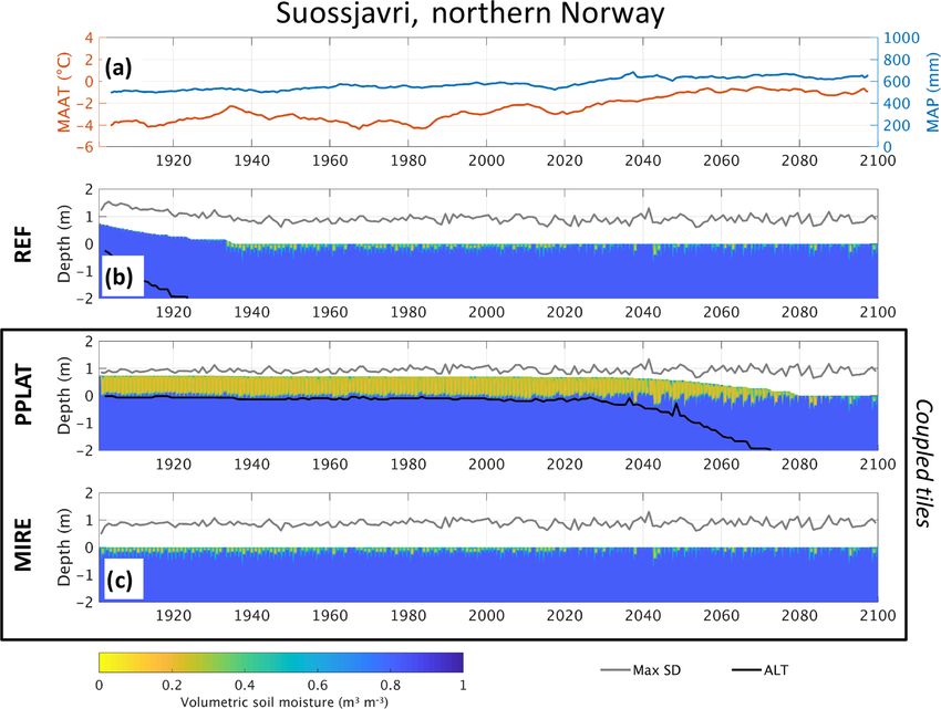
592                                                     K. S. Aas et al.: Ice-rich permafrost landscapes represented with tiles

and associated changes in the biogeochemical cycles, is             tion of peat plateaus in Canada and Sweden, respectively.
therefore important for future estimates of climate change          Although they capture different aspects of lateral fluxes in
(Schuur et al., 2015).                                              ice-rich permafrost landscapes, these simulations have been
   Comprehensive Earth system models (ESMs) are our pri-            performed with models operating on high-resolution grids,
mary tools for estimating future climate change, including          which are not transferable to large-scale land surface models
the magnitude and interplay among different climate feed-           (LSMs). Furthermore, these studies have not included mi-
backs. Due to the possibly large impact of the permafrost–          crotopography changes to represent transient landscape evo-
carbon feedback (PCF) on the climate system, permafrost             lution, which should be treated in a unified way that can be
processes have received significant attention in the devel-         applied to both continuous and discontinuous/sporadic per-
opment of these models during the last decade. Consider-            mafrost features.
able improvements have been made by including freeze–                  On the larger scale, Lee et al. (2014) included excess
thaw processes, multilayer soil carbon representation, in-          ground ice in a global LSM simulation that estimated land
creased soil depth and resolution, moss representation, and         subsidence related to permafrost thaw and ground ice melt,
multilayer snow schemes (Lawrence and Slater, 2005; Koven           but without including subgrid-scale variations and related
et al., 2013b; Chadburn et al., 2015; Burke et al., 2013).          lateral fluxes. Qiu et al. (2018) included a separate subgrid
However, the representation of subgrid-scale permafrost pro-        tile in an LSM receiving surface runoff from the surround-
cesses remains a major limitation of these models (Lawrence         ing tiles to simulate peatlands with related carbon, moisture,
et al., 2012; Beer, 2016). In particular, the ability to simulate   and energy fluxes. Gisnås et al. (2016) and Aas et al. (2017)
changing microtopography resulting from melting of excess           used subgrid tiles to represent heterogeneous snow accumu-
ground ice (thermokarst) is lacking. These processes are cur-       lation and showed how this influenced soil thermal regime
rently observed many places in the Arctic: in polygonal tun-        and surface energy fluxes, respectively. Finally, Langer et
dra, Liljedahl et al. (2016) have documented the transition of      al. (2016) employed a two-tile approach to simulate lateral
low- and flat-centered polygons (LCPs and FCPs) to high-            heat exchange in polygonal tundra, showing that heat loss
centered polygons (HCPs), with large associated changes in          to surrounding land masses was required to simulate stable
local and regional hydrology. Conversely, sporadic or iso-          thermokarst ponds in northern Siberia.
lated permafrost features like palsas and peat plateaus are            In this study, we extend the two-tile approach of Langer et
only maintained through small-scale elevation differences           al. (2016) with lateral fluxes of snow and subsurface water
and lateral fluxes of snow and water (Seppälä, 2011). Melting       flow, and we combine this with the excess ice formulation
of excess ice in these features sets off a feedback mechanism       of Lee et al. (2014). In this way, we can dynamically simu-
through subsidence, enhanced snow accumulation, reduced             late changing microtopography, which impacts lateral fluxes
winter heat loss, and increased soil ice melt, which cannot be      of snow, water, and heat. We thereby aim to simulate land-
represented in a single large-scale grid cell. Accounting for       scape changes due to excess ground ice melt in a framework
these processes in ESMs is of particular importance since the       suitable for implementation in ESMs. We apply this laterally
regions with high amounts of excess ice largely coincide with       coupled two-tile system to a polygonal tundra site in north-
areas with high amounts of soil carbon. Olefeldt et al. (2016)      ern Siberia and a peat plateau in northern Norway, and we
estimated that 20 % of the northern permafrost region is cov-       compare with results from a standard 1-D reference simu-
ered by thermokarst landscapes but suggested that as much           lation. The two sites represent cold, continuous permafrost
as 50 % of the soil organic carbon (SOC) in this region could       and warm, sporadic permafrost. Signs of permafrost degra-
be stored here.                                                     dation are currently observed at both locations, and small-
   Painter et al. (2013) described the challenges of capturing      scale heterogeneity in soil moisture and snow accumulation
the hydrologic response of degrading permafrost, partition-         is a common feature for the two locations. Hence, they repre-
ing these processes into “subsurface thermal/hydrology, sur-        sent two very different climatic conditions for which current
face thermal processes, mechanical deformation, and over-           large-scale models fail to capture key small-scale processes
land flow processes”. Some of these have been addressed             that are important for the soil thermal regime. Aiming for a
in individual studies on local scales. For instance, polygonal      proof of concept rather than capturing the detailed proper-
tundra in Alaska has been simulated by Kumar et al. (2016)          ties at the test sites, we explore the capability of the simple
using a multiphase 3-D thermal hydrology model (PFLO-               two-tile system to represent observed landscape changes and
TRAN), by Grant et al. (2017), who included lateral fluxes          related water and energy fluxes.
of subsurface water as well as redistribution of snow and
surface water, and by Bisht et al. (2018), who simulated
a 104 m long transect with submeter resolution including
snow redistribution and lateral water and energy fluxes. In
the warmer (discontinuous and sporadic) permafrost zones,
Kurylyk et al. (2016) and Sjöberg et al. (2016) included
groundwater flow and related heat advection in the simula-

The Cryosphere, 13, 591–609, 2019                                                        www.the-cryosphere.net/13/591/2019/
K. S. Aas et al.: Ice-rich permafrost landscapes represented with tiles                                                               593

                                                                         land, including investigations of water and surface energy
                                                                         balance (Boike et al., 2008; Langer et al., 2011a, b) and
                                                                         carbon cycling (Knoblauch et al., 2018, 2015). As a well-
                                                                         studied site with available meteorological, soil physical, and
                                                                         hydrological measurements (Boike et al., 2018), it has also
                                                                         been used as a test site for various permafrost modeling stud-
                                                                         ies, including ESM validation and development (Chadburn et
                                                                         al., 2015, 2017; Ekici et al., 2014, 2015).

                                                                         2.2   Suossjavri, northern Norway

                                                                         Suossjavri (69◦ 230 N, 24◦ 150 E) is situated in the central part
                                                                         of Finnmark county in northern Norway. It is part of the
                                                                         sporadic permafrost zone in northern Fennoscandia (Fig. 1),
                                                                         where permafrost outside mountain regions is confined to
                                                                         palsas and peat plateaus in mires. The site has an elevation of
Figure 1. (a) Location of the two test sites on top of the map of per-   approximately 335 m a.s.l. and covers about 23 ha. It is bor-
mafrost distribution in the Arctic (Brown et al., 1997). (b) Exam-       dered by the Iesjoka River in the south and the Suossjavri
ple of low-centered polygons on Samoylov Island, northern Siberia        Lake in the east and north and consists of palsas and peat
(photo: Sebastian Zubrzycki). (c) Example of peat plateau near Su-       plateaus that rise up to 2 m above the surrounding wet mire.
ossjavri, northern Norway (photo: Sebastian Westermann). The two         These permafrost features are degrading strongly, having lost
sites are located in the continuous and sporadic permafrost zones.       approximately 30 % of their area in the last 6 decades (Borge
                                                                         et al., 2017). The largest degradation rates are seen for the
                                                                         smaller palsas and peat plateaus, which have lost almost half
2     Methods
                                                                         of their area in this period, compared to only 15 % aerial loss
                                                                         of the larger peat plateaus.
2.1     Site descriptions
                                                                            The mean annual air temperature in the region ranges
The model is applied to the two permafrost locations shown               from −2 to −4 ◦ C, with a summer mean value of 10 ◦ C
in Fig. 1. Samoylov Island in northern Siberia represents a              (JJA) and winter value of −15 ◦ C (DJF; Aune, 1993, for
polygonal tundra location in cold, continuous permafrost,                the 1961–1990 period). The mean annual precipitation is be-
while peat plateaus in Suossjavri, northern Norway, repre-               low 400 mm according to the nearest measurement station
sent warm, sporadic permafrost. Both locations are, however,             (Borge et al., 2017). Mean annual ground surface tempera-
examples of carbon- and ice-rich permafrost landscapes in                tures (MAGSTs) have been measured with iButton® temper-
which small-scale lateral fluxes of water, heat, and snow are            ature loggers at 25 locations since September 2015, in con-
known to occur.                                                          junction with end-of-summer thaw depths and end-of-winter
                                                                         snow depths at the same points. These show snow depths on
2.1.1    Samoylov Island, northern Siberia                               the peat plateaus mostly between 0 and 40 cm, an active layer
                                                                         thickness (ALT) between 40 and 70 cm, and 1 to 2 ◦ C colder
Samoylov Island (72◦ 220 N, 126◦ 280 E) is located in the                MAGSTs compared to the surrounding wet mire areas.
southeast corner of the Lena River delta. The size of the
entire Delta, including more than 1500 islands and about                 2.3   The Noah-MP land surface model
60 000 lakes, is about 25 000 km2 (Fedorova et al., 2015),
and the area is underlain by continuous cold permafrost.                 The modeling study is performed with the Noah-MP LSM
The island of Samoylov, located in the southern part of the              version 3.9, with a number of modifications described be-
delta, mainly consists of polygonal tundra with a number                 low. In its default configuration the Noah-MP model (Niu
of ponds and lakes (Fig. 1b; Boike et al., 2013, 2018). All              et al., 2011) simulates soil temperature and frozen and liq-
degradation stages described by Liljedahl et al. (2016) can              uid water in four soil layers down to a depth of 2 m. It
be found here, from non-degraded LCPs to HCPs with con-                  includes up to three snow layers with a representation of
nected troughs (see Nitzbon et al., 2018). Between 1997 and              liquid water retention and refreezing, as well as a separate
2017, the mean annual air temperature at the island was ap-              canopy layer. Compared to the original Noah code, Noah-MP
proximately −12.3 ◦ C, with an annual liquid precipitation of            is an augmented version that includes multiple alternative
169 mm and mean end-of-winter snow depth of 0.3 m (Boike                 model representations for key processes, including parame-
et al., 2018). At the depth of zero annual amplitude (20.8 m),           terizations of supercooled liquid water and frozen ground hy-
the permafrost had warmed from −9.1 ◦ C in 2006 to −7.7 ◦ C              draulic conductivity (see details in Niu et al., 2011). It is sub-
in 2017. Numerous studies have been conducted on the is-                 stantially less complex and computationally expensive than

www.the-cryosphere.net/13/591/2019/                                                               The Cryosphere, 13, 591–609, 2019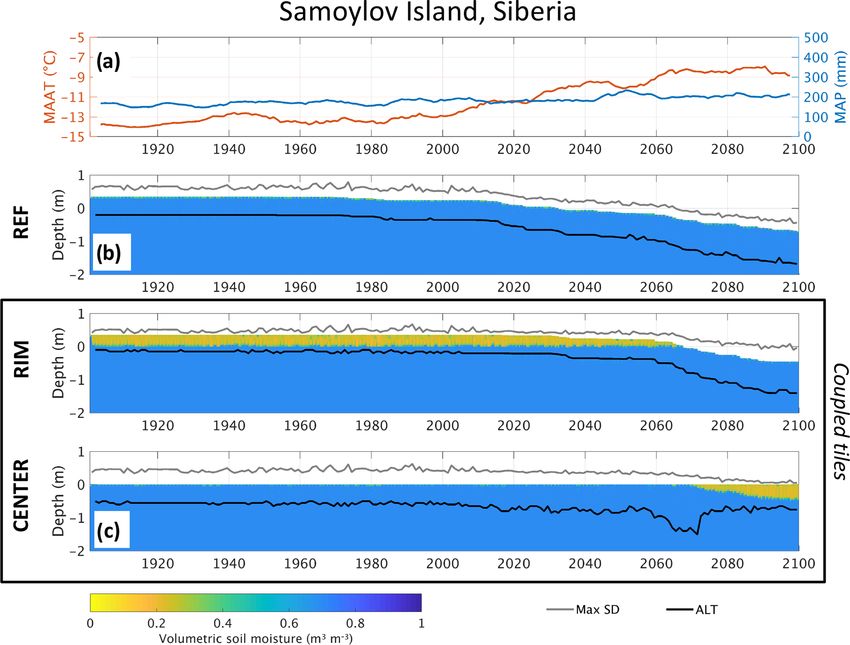
594 K. S. Aas et al.: Ice-rich permafrost landscapes represented with tiles
LSMs used in current state-of-the-art ESMs, lacking for in-
stance representations of biogeochemical processes and dy-
namical vegetation. However, in its basic treatment of soil
thermal and hydrological processes, it is comparable to, and
includes some of the same parameterizations as, the Com-
munity Land Model (CLM; Lawrence et al., 2011). Fur-
thermore, lateral subsurface water fluxes are already imple-
mented in this model as part of the WRF-Hydro modeling
system (see Sect. 2.2.4). With some modifications it is there-
fore a suitable base model for studying the geophysical as-
pects of permafrost thaw, including the importance of lateral
fluxes. In the following, we will describe the modifications
and augmentations to the Noah-MP model for our simula-
tions.
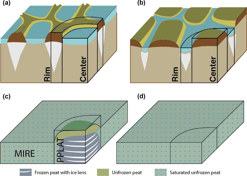
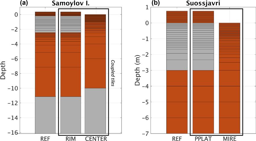
2.3.1 Soil resolution, excess ice, and soil organic Figure 2. (a) Schematic presentation of non-degraded low-centered
fraction polygons (left) and degraded high-centered polygons (right) with
corresponding tiles used in this study (adapted from Liljedahl et
To better represent permafrost processes, the number of soil al., 2016). (b) Schematic presentation of peat plateau in a surround-
layers was increased from the default four to 37, with the ing mire (left), and the mire after the peat plateau has degraded
total soil depth increasing from 2 to 7 or 14 m, plus excess (right), with corresponding tiles.
ice thickness (Fig. A1). These soil depths were chosen to ap-
proximately include the zero annual amplitude depth at Su-
ossjavri and Samoylov but still be shallow enough to avoid tiles, we will refer to these as tiles 1 and 2, but later we refer
long spin-up times, as the emphasis of this work is on near- to them as RIM and CENTER for the polygonal tundra and
surface processes rather than deep soil conditions. PPLAT and MIRE for the peat plateau setting (Fig. 2).
Secondly, we added soil organic fraction as an additional
(fixed) input variable. Following Lawrence and Slater (2008), 2.3.3 Snow redistribution between interactive tiles
soil thermal and hydraulic properties were calculated assum-
ing a linear weight between organic and the (original) min- To represent the effect of snow redistribution by wind, we
eral fractions. This facilitated simulating organic rich soils scale the amount of snow received in tiles 1 and 2 based on
like peat whose properties are different from the default soil the difference in elevation at the top of the snow or soil col-
types available in Noah-MP. umn. Similar to Aas et al. (2017), this is performed with a
Following Lee et al. (2014), we included excess ice within scaling factor, so that the accumulation of snow in tile i is
the existing layers of the model, so that the layer thicknesses calculated according to the grid-cell mean snowfall S times
and properties of the layers change throughout the simulation the scaling factor fi (Si = fi · S).
as the excess ice melts. Excess ice is initialized as a certain The scaling factor is calculated as follows: for snow depths
fraction (Fexice ), within a certain depth region in each soil below a minimum snow value (Hsmin ), no redistribution takes
column (see Figs. 3 and A1). Because excess ice is incorpo- place, i.e.,
rated as an initial condition, it only melts and does not grow.
The water from melting excess ice is added to the soil col-
fi = 1.0, for Hsi < Hsmin . (1)
umn in the layer where it melts or the nearest unsaturated
layer above if this layer is saturated.
Once the tile with the highest elevation reaches the minimum
2.3.2 Implementation of interacting tiles snow value, the scaling factor is calculated so that no new
snow accumulates on this tile before the total snow and soil
Subgrid tiles have been implemented in the original Noah elevation (zi ) are within 5 cm of each other:
version as part of the Weather Research and Forecasting
(WRF) model to represent a mosaic of land cover types (Li
1.0, for |z1 − z2 | < 0.05
m
0.0, for z1, 2 − z2, 1 ≥ 0.05 m
et al., 2013). This tiling included soil columns simulated in- f1, 2 = , (2)
dependently for each tile, but without any interaction be- A2, 1
1.0 + , for z2, 1 − z1, 2 ≥ 0.05 m
tween the tiles during the simulation. Here we build upon A1, 2
this methodology to explicitly simulate individual land units
within a grid cell, but also include lateral fluxes as described where A refers to the area of the tile, and the subscript refers
below. In the following general description of the interactive to the tile number (1 or 2).
The Cryosphere, 13, 591–609, 2019 www.the-cryosphere.net/13/591/2019/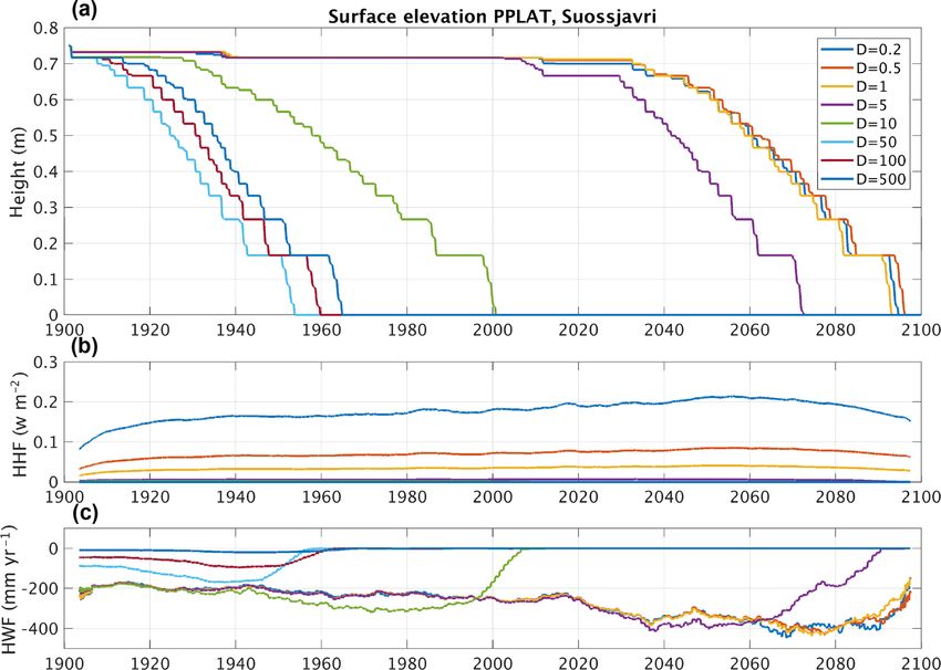
K. S. Aas et al.: Ice-rich permafrost landscapes represented with tiles 595
2.3.4 Lateral subsurface water flux between interactive
tiles
Lateral water flux is calculated similar to subsurface flow in
WRF-Hydro (Gochis et al., 2015), with a few modifications
relevant for permafrost conditions. The flow rate (m3 s−1 )
from one tile to another can be calculated as
−T tan (β) L, for β < 0
q= , (3)
0, for β ≥ 0
where T is the transmissivity, L is the contact length, and β Figure 3. Schematic presentation of the two-tile system with ge-
is the water table slope between the tiles. T is given by ometry parameters. Parameter values used for the two locations are
listed in Table 1.
zwt n
Ksat, 0 ZB
1− , for zwt ≤ ZB
T = n ZB . (4)
0, for zwt > ZB
symmetry). At both locations, a separate reference simula-
tion (REF) is run with the same initial conditions as the el-
Here zwt is the water table depth, ZB is depth to the bottom of evated tile in the laterally coupled system (RIM or PPLAT),
the soil column, Ksat, 0 is the saturated hydraulic conductivity corresponding to the same model setup as employed in Lee
at the surface, and n is a tunable local power-law exponent et al. (2014), i.e., a 1-D excess ice representation without lat-
determining the decay rate of Ksat with depth. eral exchange. The other (initially lower) tile in the laterally
Here we set n = 1 and use the depth to the minimum (high- coupled simulation is referred to as CENTER and MIRE for
est) frost table depth (zfrzmin ) instead of the full soil depth the tundra and mire locations, respectively.
zwt −zwt
ZB . Inserting tan (β) = 1, 2 D 2, 1 , where D is the distance
parameter, the flow rate can then be calculated as 2.4.1 Polygonal tundra on Samoylov Island, northern
Siberia
zwt − zwt2, 1
−W Ksat 1, 2
(zfrzmin − zwtmin ) ,
q1, 2 = D . (5) The polygonal landscape at Samoylov Island is represented
for zfrzmin ≥ zwtmin
by two tiles that represent center and rim areas. These are in
0, for zfrzmin < zwtmin
reality different sizes and shapes (Fig. 1) but can to a first
Here we set the frost table to the top of the first layer (from approximation be considered a self-repeating pattern, as also
the top) with more than 1 % volumetric soil ice (including described by Nitzbon et al. (2018). Due to symmetry, a larger
excess ice). The water table depth is taken as the depth to the region can then be represented as a single feature with a rep-
top of the first saturated soil layer. resentative geometry, neglecting the interaction between dif-
ferent polygons. For simplicity, here we simulate a represen-
2.3.5 Lateral heat flux between interactive tiles tative polygon as a circular feature with a center and rim of
equal area and a total diameter of 10 m. Assuming hexagons
The lateral ground heat flux (W m−2 ) between two tiles with instead of circles, like Nitzbon et al. (2018), would only re-
overlapping soil depth of 1z can be calculated as (see Langer quire minor modifications to the parameters shown in Fig. 3,
et al., 2016) particularly the distance parameter and the interaction length.
To represent an ice wedge occupying the majority of the
L T2, 1 − T1, 2
qs1, 2 = ks 1z, (6) soil volume, we initialize the RIM tile with an excess ice
A1, 2 D fraction of two-thirds between the simulated ALT at 55 cm
where ks is the thermal conductivity. This is calculated indi- and 2.8 m below the surface, which expands the soil thick-
vidually for each partially overlapping soil layer. ness of the RIM by 1.5 m. To allow the RIM to sink below
the elevation of the center, we add excess ice to the bottom
2.4 Model setup and forcing soil layer, with the largest amount in CENTER, so that the
total elevation difference is only 35 cm (Fig. A1). This is
The model setup is shown in Fig. 3 and Tables 1 and 2 and de- an approximate average value for observed rim heights at
scribed separately for the two locations in the following, to- Samoylov. The model is initialized with a soil temperature of
gether with the forcing data for the corresponding locations. −9 ◦ C and fully saturated and frozen soil throughout the col-
In both cases, a model time step of 15 min is applied, with umn. While this is substantially colder than the equilibrium
zero flux as the lower thermal boundary condition. To rep- temperature reached by the model, the soil temperatures in
resent larger-scale landscapes with a small number of tiles, the lowest cell (lower boundary at ca. 16 m, i.e., 14 m plus
we exploit the concept of self-similarity (i.e., translational 2.15–2.5 m excess ice) reach an equilibrium within the first
www.the-cryosphere.net/13/591/2019/ The Cryosphere, 13, 591–609, 2019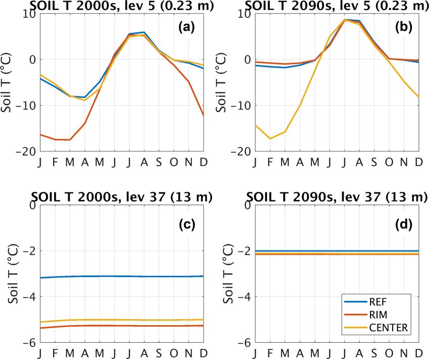
596                                                                 K. S. Aas et al.: Ice-rich permafrost landscapes represented with tiles

Table 1. Tile geometry and excess ice distribution. See details in Fig. 3.

                             Location                Ar       Ac         L      D       e       Zextop   Zexbot   Fexice
                                                   (m2 )     (m2 )      (m)    (m)     (m)       (m)       (m)     (%)
                             Sam                  39.3       39.3      22.2   4.27     0.35      0.55      2.8    66.7
                             Suo            9.92 × 10³       78.5      31.4   10.0     0.75      0.75     3.75    25.0

Table 2. Soil properties and initial conditions.                                larger features (see Sect. 4.2), and more complex geome-
                                                                                tries can be represented by applying appropriate distance and
 Location     OrgF     Scenario        T0     Hsmin        Pscale     Soil      contact length parameters. As the mire does not contain per-
              (%)                   (◦ C)      (m)                    type      mafrost, only the peat plateau tile (PPLAT) was initiated with
 Sam           50      RCP4.5       −9.0       0.05         0.6       Silt      excess ice (Fig. A1b), starting 75 cm below the surface with a
 Suo           80      RCP4.5        0.0        0.1         1.0       Silt      total excess ice thickness of 75 cm distributed down to 3.75 m
                                                                                below ground. Both tiles were started from fully saturated
                                                                                conditions and 0 ◦ C soil temperatures. The soil water was
                                                                                initially unfrozen in all soil layers, except for the ones con-
decade of the simulation (mean increase of 0.3 ◦ C yr−1 ), after                taining excess ice, in which soil (pore) water was initially
which the annual changes vary between positive and negative                     frozen.
values.                                                                            Forcing data for this location were generated in a similar
   As model forcing for the Samoylov Island simulation, we                      way as the data used at Samoylov Island. CRU-NCEP data
used the same model input as Westermann et al. (2016). This                     from the nearest grid point were used for the historical part,
is based on the CRU-NCEP data for the historical period                         while anomalies for the future (starting in year 2010) were
(1901–2015; Viovy, 2018). For the future part of the simula-                    taken from CCSM4 simulation following the RCP4.5 sce-
tion, this dataset uses model output from the CCSM4 climate                     nario and added or multiplied to the reference period 1996–
model following the mitigation scenario RCP4.5, to calculate                    2005.
monthly climate anomalies for temperature, humidity, pres-
sure, and wind and scaling factors for precipitation and radi-
ation. These are added or multiplied to the high-frequency                      3     Results
data from 1996 to 2005 from the historical (CRU-NCEP)
data, following Koven et al. (2015). The RCP4.5 scenario                        In the following, we outline the model results for the polyg-
was chosen as it represents a strong mitigation scenario but                    onal tundra site in northern Siberia (Sect. 3.1) and the peat
still shows continued warming in the Arctic throughout the                      plateau location in northern Norway (Sect. 3.2).
21st century, which makes understanding permafrost pro-
cesses highly relevant.                                                         3.1    Samoylov Island, northern Siberia
   Detailed measurements of snow accumulation from eight
LCPs from 2008 showed average snow depths of 17 cm on                           During the simulation period, Samoylov Island experiences a
the rims and 46 cm in the centers, with a total average snow                    strong increase in annual mean air temperature and a modest
water equivalent (SWE) of 65 mm (Boike et al., 2013). As                        increase in precipitation (Fig. 4a). Mean air temperatures in-
the model accumulated too much snow compared to these                           crease from approximately −14 ◦ C in the early 20th century
observations due to a bias in the precipitation forcing (West-                  to about −8 ◦ C towards the end of the 21st century (RCP4.5
ermann et al., 2016), we scaled the precipitation with a con-                   scenario), with most of the warming occurring in the 21st
stant factor (Pscale ) of 0.6 throughout the simulation in order                century.
to simulate realistic SWE and snow depths.                                         Both the reference and the laterally coupled simulations
                                                                                show stable permafrost with ALT between 0.45 and 0.65 m
2.4.2   Peat plateaus in Suossjavri, northern Norway                            during the historical period of the simulation (until 2010).
                                                                                This is in good agreement with observations, showing mean
Similar to the polygonal tundra, the peatland of Suossjavri                     ALT close to 0.5 m (Boike et al., 2013, 2018). For snow depth
is represented with two interacting land units. In this case                    and near-surface soil moisture conditions, the laterally cou-
we represent a single circular peat plateau with a diame-                       pled simulations show clear differences from REF (Fig. 4b
ter of 10 m, corresponding to the smaller features observed                     and c) and mimic the observed conditions more closely (see
in the study area. This is placed in a significantly larger                     Boike et al., 2013, 2018, and Nitzbon et al., 2018). The sim-
(100 m × 100 m) surrounding mire, so that the effect of the                     ulated maximum snow depths in 2008 compare well with ob-
coupling mainly affects the elevated tile. The areas of both                    servations for both RIM (0.23 m compared to 0.16 m) and the
the mire and the peat plateau can be increased to represent                     centers (0.39 m compared to 0.46 m), although the observa-

The Cryosphere, 13, 591–609, 2019                                                                        www.the-cryosphere.net/13/591/2019/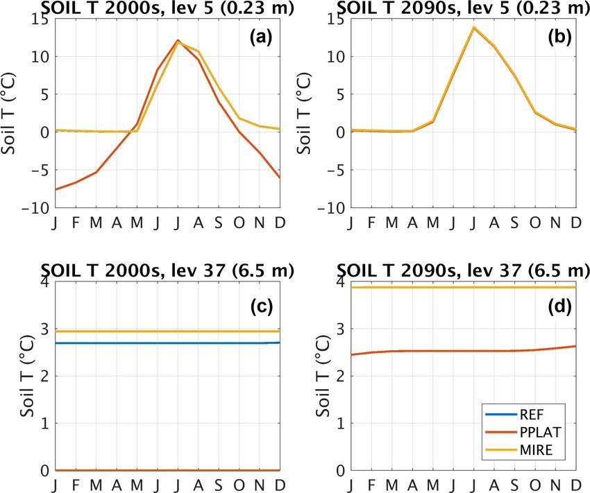
K. S. Aas et al.: Ice-rich permafrost landscapes represented with tiles 597
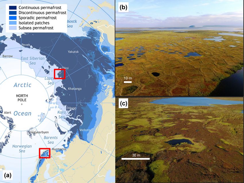
Figure 4. (a) The 10-year running average of mean annual air
temperature (MAAT) and mean annual precipitation (MAP) at
Samoylov Island. Soil moisture and surface elevation are shown as Figure 5. Average annual temperature cycle during the first (a, c)
colored regions in (b) the reference simulation (c) and in the lat- and last (b, d) decades of the 21st century at Samoylov Island, in the
erally coupled tiles. Note that both the surface elevation (relative fifth model layer (a, b; 0.23 m below surface) and the 37th model
to the CENTER tile) and the unsaturated soil (orange and green) layer (c, d; approximately 13 m below reference height). See layer
change in the coupled tiles as excess ice melts and the lateral fluxes depths in Fig. A1a.
change. Maximum annual snow depth (MaxSD) and active layer
thickness (ALT) are shown as gray and black lines, respectively.
tions (Boike et al., 2018). At depth, the soil temperatures are
higher than observed, with values of around −3 ◦ C in REF
tions show a considerable spread (see Nitzbon et al., 2018). and −5 ◦ C in the laterally coupled simulation, compared to
This was partly achieved by applying a scaling factor for pre- −8.6 ◦ C at 10.7 m in depth observed during the second half
cipitation (Pscale ) of 0.6 (Table 2). In agreement with obser- of this decade (Boike et al., 2013). Here it is worth noticing,
vations (see Chadburn et al., 2017, and Nitzbon et al., 2018), however, that these temperatures have increased more than
the model displays dry near-surface soil conditions in the 1 ◦ C during the last decade (Boike et al., 2018).
RIM and mostly saturated conditions in the CENTER tile, Again, clear differences can be seen between REF and the
which cannot be represented in the REF simulation. With in- laterally coupled tile system. In the current climate (Fig. 5a,
creasing air temperatures in the 21st century, the ALT deep- c), REF and CENTER show a very similar annual cycle,
ens and surface subsidence occurs in REF, reaching 35 cm whereas the amplitude of the temperature cycle is much
around 2030 and more than 1 m by the end of the century. In larger in RIM. In the active layer, the difference is almost
the two-tile simulation, RIM remains relatively stable and el- exclusively observed during winter, when the effect of shal-
evated above the center until around 2070, almost 4 decades lower snow depth is decreasing the winter insulation in RIM.
later than REF. RIM subsequently subsides due to excess ice Deeper in the soil column the differences in soil tempera-
melt, eventually sinking below CENTER, which marks the ture become less pronounced between the two coupled tiles
transition from LCP to HCP. Towards the end of the simula- (RIM and CENTER), as heat exchange between the tiles be-
tion RIM appears to stabilize with a subsidence of 80 cm and comes more important. In the deep soil (Fig. 5c) the tempera-
an ALT of less than 1 m, in contrast to the single-tile REF. ture is similar (within 0.5 ◦ C), but around 2 ◦ C colder than in
CENTER experiences ALT deepening in the 21st century, REF. At the end of the century (Fig. 5b), the situation has re-
which reaches a maximum around 2070. The deepening of versed and the now elevated, dry CENTER with low snow ac-
the active layer follows the rapid increase in forcing temper- cumulation features cold winter temperatures, whereas RIM
ature and lasts until RIM has subsided below CENTER. After largely follows REF. Deeper in the soil, the two coupled tiles
this point the elevated RIM tile has turned into a trough, and are again colder than REF, although the difference is smaller
the top layers in CENTER start to drain, resulting in shal- than in the beginning of the century (Fig. 5d). Comparing the
lower ALT. This marks the transition from a LCP to a HCP. temperatures at 2 m in depth from the surface in REF and the
Soil temperatures. The annual cycle of the soil tempera- area-weighed mean of the two coupled tiles (here mean of
ture is shown in Fig. 5. In the current climate (Fig. 5a, c), RIM and CENTER), we find the coupled simulation on av-
the elevated rim shows annual temperature variations in the erage 2.1 ◦ C colder than REF during the 20th century. This
active layer of more than 20 ◦ C, in agreement with observa- difference decreases to almost zero during the transition from
www.the-cryosphere.net/13/591/2019/ The Cryosphere, 13, 591–609, 2019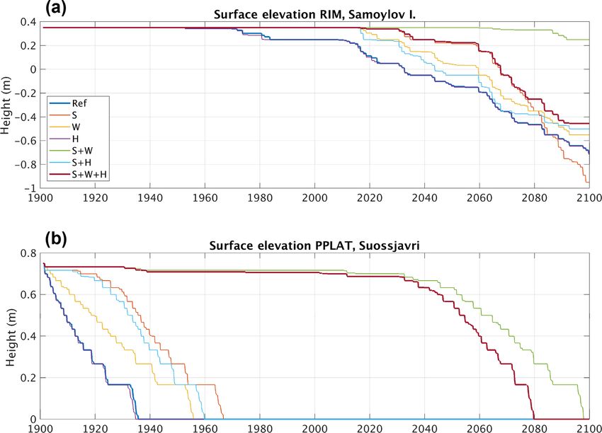
598                                                          K. S. Aas et al.: Ice-rich permafrost landscapes represented with tiles

                                                                             Qualitatively, our simulation captures the observed differ-
                                                                          ence between the RIM and CENTER reported by Langer et
                                                                          al. (2011b), although the simulation seems shifted towards
                                                                          higher SH fluxes and lower LH fluxes. This again might be
                                                                          related to too low water holding capacity in our simulations,
                                                                          as well as the lack of surface water on top of the LCP.

                                                                          3.2   Suossjavri, northern Norway

                                                                          Figure 7 shows the soil moisture, surface elevation, ALT,
                                                                          and snow depth at the mire location in the sporadic per-
                                                                          mafrost zone in northern Norway. In REF, permafrost starts
                                                                          to degrade at the beginning of the simulations, with excess
                                                                          ice rapidly disappearing during the first 3–4 decades of the
                                                                          simulation. After this point, REF has turned into a mostly
                                                                          saturated wetland with maximum snow depths of around
Figure 6. Summer surface energy fluxes at Samoylov Island during          1 m. The corresponding tile in the laterally coupled system
the first (a) and last (b) decades of the 21st century in the reference   (PPLAT) experiences low maximum snow depths and dry
simulation (REF) and laterally coupled tiles (RIM and CENTER).            surface conditions (Fig. 7c), which results in a thermally sta-
SH: sensible heat flux; LH: latent heat flux; GRDFLX: ground heat         ble peat plateau throughout the 20th century. Compared to
flux.
                                                                          observations at this location (see Sect. 2.1.2), the PPLAT
                                                                          shows a somewhat larger ALT (0.75–0.9 m) in the histori-
                                                                          cal period. The initial excess ice does not start to melt until
LCP to HCP, before the coupled simulation becomes 1.4 ◦ C                 around 2030, when both air temperatures and precipitation
colder during the final 2 decades of the simulation.                      start to increase rapidly. Accelerating ALT deepening in con-
   Summer surface energy fluxes. A clear difference between               junction with surface subsidence due to excess ice melt is
the tiles is seen in the summer surface energy fluxes (Fig. 6).           seen after 2050, when the mean air temperature has stabilized
As expected, the dry RIM shows larger sensible heat (SH)                  at about −1 ◦ C and precipitation at around 650 mm. This pro-
and lower latent heat (LH) fluxes than REF before degrada-                cess appears to be driven by feedbacks in the system: as the
tion, whereas the wet CENTER shows the opposite (Fig. 6a).                ALT deepens and excess ice melts, the peat plateau subsides,
This is reversed in the degraded state when CENTER is                     leading to more snow remaining in this tile and smaller heat
dry and the trough (subsided RIM tile) is wet. Interestingly,             loss during winter, which again enhances summer melt. Fur-
the landscape aggregated values (here the mean of RIM and                 thermore, the subsidence also results in a thinner layer of
CENTER) is only a few watts per square meter different from               dry peat as the water table is largely controlled by the ele-
the reference for these two fluxes both before and after degra-           vation relative to the surrounding wet mire, which lowers the
dation (Fig. 6a, b). We note, however, that this depends on               insulation during summer. Combined with the direct effect
drainage conditions. Here only surface water (infiltration ex-            of water from the excess ice melt increasing the soil mois-
cess) is removed as runoff, whereas advanced degradation of               ture in PPLAT, this leads to a melt–subsidence–soil moisture
this kind of polygons is often associated with drainage also of           feedback, in addition to the melt–subsidence–snow feedback.
the troughs (Liljedahl et al., 2016). This effect is not included         The surrounding MIRE is largely unaffected by the presence
here but is simulated and discussed by Nitzbon et al. (2018)              and disappearance of the elevated peat plateau as it is as-
and would likely increase the Bowen ratio of laterally cou-               sumed to be about 2 orders of magnitude larger. Hence, REF
pled tiles in the degraded stage compared to both REF and                 and MIRE develop very similarly after the initial excess ice
the non-degraded stage. It is also likely that the difference             in REF has melted.
between the reference simulation and the aggregated values                   Soil temperatures. The soil temperatures in the laterally
would be larger with a different areal fraction of RIM com-               coupled tiles differ substantially in the present non-degraded
pared to CENTER.                                                          state (Fig. 8a, c). While REF and MIRE have nearly identical
   The ground heat flux (GRDFLX) is lower during both time                annual temperature cycles near the surface, PPLAT deviates
periods for the mean of the two coupled tiles than the REF,               in several points. First, the elevated PPLAT shows cold win-
due to a substantially reduced flux in the dry, elevated tile             ter soil temperatures (as low as −7.6 ◦ C in January), com-
(first RIM, then CENTER). This points to the effect of dry                pared to a constant, 0 ◦ C temperature in MIRE and REF. Fur-
peat insulating the soil and suggests that the lower tempera-             thermore, PPLAT responds quicker to the onset of both sum-
tures in the laterally coupled system could be a result of both           mer and winter, with both MIRE and REF shifted to warmer
increased summer insulation as well as the reduced winter                 temperatures in late summer and colder temperatures dur-
insulation mentioned above.                                               ing spring. One key factor controlling these differences is

The Cryosphere, 13, 591–609, 2019                                                              www.the-cryosphere.net/13/591/2019/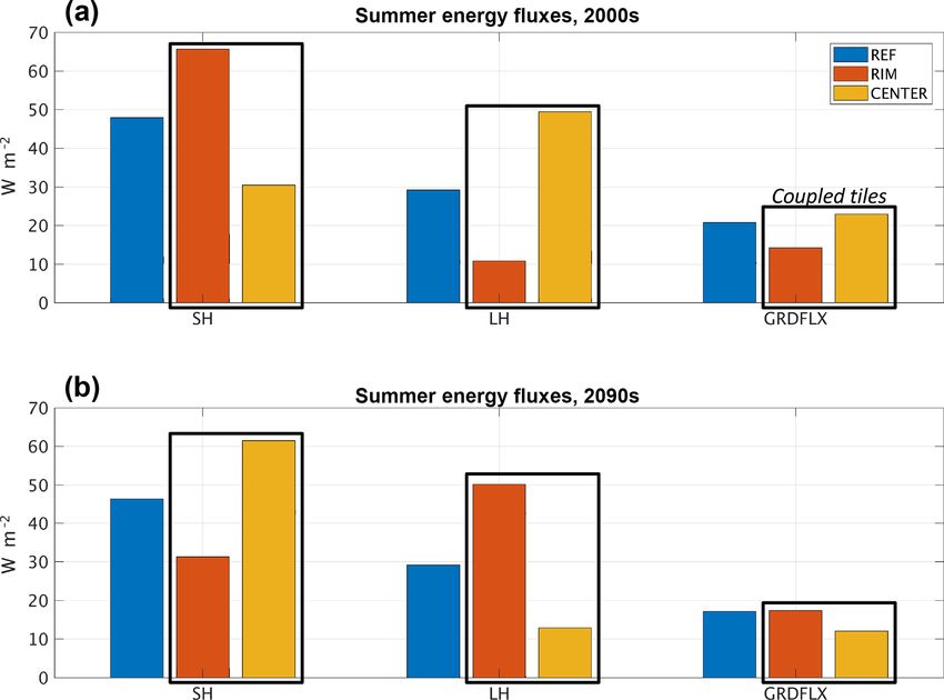
K. S. Aas et al.: Ice-rich permafrost landscapes represented with tiles                                                                 599

Figure 7. (a) The 10-year running average of mean annual air
temperature (MAAT) and mean annual precipitation (MAP) at Su-
ossjavri, northern Norway. Soil moisture and surface elevation are       Figure 8. Average annual temperature cycle during the first (a, c)
shown as the colored region in (b) the reference simulation (c) and      and last (b, d) decades of the 21st century at Suossjavri, northern
in the laterally coupled tiles. Note that both the surface elevation     Norway, in the fifth model layer (a, b; 0.23 m below surface) and
(relative to the CENTER tile) and the unsaturated soil (orange and       the 37th model layer (c, d; 6.5 m below reference height). See layer
green) change in the coupled tiles as excess ice melts and the lateral   depths in Fig. A1b.
fluxes change. Maximum annual snow depth (MaxSD) and active
layer thickness (ALT) are shown as gray and black lines, respec-
tively.

the low snow accumulation in PPLAT, which leads to both
an increased annual temperature cycle near the surface and
earlier snow melt. Another factor is the higher soil moisture
in REF and MIRE (both mostly saturated), which due to the
high heat capacity of water delays the soil response to chang-
ing atmospheric temperatures.
   Below the depth of zero annual amplitude, PPLAT dis-
plays warm permafrost conditions at 0 ◦ C, whereas the MIRE
and REF feature temperatures close to 3 ◦ C. The REF simu-
lations are about 0.25 ◦ C colder than MIRE, which is most
likely a legacy of excess ice melt earlier in the simulation
(Fig. 7).
   After degradation (Fig. 8b, d), differences among the three           Figure 9. Summer surface energy fluxes at Suossjavri, northern
realizations are marginal near the surface. At this point, there         Norway, during the first (a) and last (b) decades of the 21st cen-
is no elevation difference, so that differences in snow accu-            tury in the reference simulation (REF) and laterally coupled tiles
mulation and other surface parameters vanish. Some differ-               (RIM and CENTER). SH: sensible heat flux; LH: latent heat flux;
ences remain in deeper soil layers, where the PPLAT tile con-            GRDFLX: ground heat flux.
tinues to warm after the ice melt.
   Summer surface energy fluxes. The different snow and soil
conditions between MIRE and PPLAT are clearly visible in                 are only marginally different from the single MIRE tile (sim-
the summer surface energy fluxes (Fig. 9). In the present non-           ilar to REF). However, observed peat plateaus can occupy a
degraded state, the PPLAT tile shows almost opposite SH and              large area of the landscape (as also seen from Fig. 1b), and
LH fluxes compared to both MIRE and REF, which again are                 configurations with larger PPLAT area would likely result in
practically identical. While the MIRE and REF both show 3                larger differences in the aggregated fluxes.
to 4 times larger LH than SH, the opposite is the case for the              For the ground heat flux (GRDFLX) the differences are
dry, elevated PPLAT. As the MIRE is 2 orders of magnitude                smaller, but still substantial. The elevated PPLAT receives on
larger than PPLAT in the model setup, the aggregated fluxes              average less energy from the surface during summer com-

www.the-cryosphere.net/13/591/2019/                                                                The Cryosphere, 13, 591–609, 2019
600                                                     K. S. Aas et al.: Ice-rich permafrost landscapes represented with tiles

pared to both RIM and MIRE. With colder temperatures at             stability (see Seppäla, 2011). Adding the lateral heat flux
depth in this tile, this points to the insulating effect of dry     to the reference setup (purple) has little effect. However, in
peat, in addition to the abovementioned winter effect due           combination with the snow and water coupling, the heat flux
to shallower snow depths. In the degraded phase, the differ-        speeds up the melt, so that the peat plateau disappears 2
ence among all three realizations has nearly vanished, as the       decades earlier than in the simulations without lateral heat
PPLAT is no longer elevated from the MIRE. Here only a              fluxes.
slightly larger GRDFLX (barely visible) shows that temper-             In conclusion, it appears that all three lateral fluxes are
atures in deeper layers have not yet reached an equilibrium.        important at both locations. Compared only to the reference
                                                                    simulation, the effect of snow redistribution is largest, fol-
                                                                    lowed by the effect of coupling through water fluxes, while
4     Sensitivity studies                                           the effect of the lateral heat flux alone is marginal. However,
                                                                    both snow and water coupling act to cool the elevated tile
To further investigate the importance of the different pro-         compared to CENTER and MIRE, as seen by the delayed
cesses in the laterally coupled system, we perform two sets of      subsidence. Hence, an increased thermal gradient between
sensitivity studies. First, we look at the effect of selectively    the different tiles is generated, which increases the effect of
activating different lateral fluxes at both locations, before in-   the lateral heat flux, reducing the stabilizing effect of snow
vestigating the effect of the distance parameter (D) for the        and water fluxes and speeding up degradation. The relative
simulation of the peat plateau.                                     effect of the different processes is therefore complex and
                                                                    must be seen in combination with the other fluxes.
4.1    Snow, water, and heat coupling                                  The influence of the different lateral fluxes is sensitive to
                                                                    process implementation and key model parameters. This is
Figure 10 shows the surface elevation in the initially elevated     especially the case for snow redistribution, which in our sim-
tiles (RIM and PPLAT) at both locations for different combi-        ulations was found to be the most important lateral process.
nations of lateral fluxes. Here, the thick blue line represents     Here, we redistribute all solid precipitation from the tile with
the reference simulation (similar to REF), whereas the sim-         the highest surface elevation (soil + snow), once a minimum
ulation with all lateral fluxes activated (similar to RIM and       snow depth is reached (Hsmin ). Increasing (decreasing) this
PPLAT) is shown with a thick red line (in the following re-         limit will decrease (increase) the effect of snow redistribution
ferred to as “fully coupled”).                                      in the simulation. An additional set of sensitivity simulations
   For the polygonal tundra site (Fig. 10a) the snow effect         with different values of Hsmin ranging from 0.0 to 0.15 m (not
alone (thin red) gives results similar to those of the fully        shown) revealed that the landscape evolution at the polygonal
coupled simulation during most of the time period. The dif-         site was relatively insensitive to this value, with the transition
ference is clear only towards the end, when the snow-only           from LCP to HCP shifting by less than 2 decades between
experiment continues to melt and subside with a trough              the minimum and maximum value. A larger sensitivity was
approaching 1 m in depth (corresponding to 1.35 m subsi-            seen for the peat plateau site, for which the lowest values of
dence), while the fully coupled system stabilizes with a            Hsmin resulted in stable permafrost throughout the 21st cen-
45 cm trough. Adding lateral water (yellow) or heat (pur-           tury. Similarly, the thermal and hydraulic conductivity of the
ple) fluxes has opposite effects, decreasing and increasing the     soil determines the effect of the heat and water fluxes, re-
melting, respectively. The snow-plus-water coupling (green)         spectively. However, the effect of lateral heat flux was only
results in an almost stable rim throughout the simulation,          important in combination with snow and/or water coupling,
subsiding only about 10 cm before the end of the 21st cen-          as there must already be a thermal gradient between the tiles
tury, whereas the snow-plus-heat coupling (thin blue line)          before it can have an effect.
results in subsidence about 10 years earlier than the fully
coupled realization, but eventually stabilizing at almost the
                                                                    4.2   Distance parameter (D)
same depth.
   At the peat plateau location in northern Norway, the
combined effect of snow and water coupling is needed to             At the peat plateau location, we performed a sensitivity anal-
simulate a stable peat plateau throughout the 20th century          ysis of the distance parameter (D), which determines lat-
(Fig. 10b). Only the fully coupled (thick red line) and the         eral water and heat fluxes are inversely proportional (Eqs. 5
snow-plus-water coupling (green) can represent stable per-          and 6). However, the water can potentially drain fast, with
mafrost, whereas all other simulations display degradation          soil water contents quickly reaching equilibrium, while the
starting within the first decades of the 20th century and           heat conduction is generally much slower. To test a wide
ground ice disappearing entirely before 1970. This is in            range of parameter values, we again simulate a circular el-
agreement with previous studies of palsas and peat plateaus         evated tile (as in Sect. 3) but scale both the elevated PPLAT
in this region, pointing to low snow accumulation and dry           and the surrounding MIRE by a factor of 100 in each hori-
peat during summer as the most important factors for their          zontal direction, testing length scales from 0.2 to 500 m.

The Cryosphere, 13, 591–609, 2019                                                         www.the-cryosphere.net/13/591/2019/
K. S. Aas et al.: Ice-rich permafrost landscapes represented with tiles 601
Figure 10. Surface elevation of RIM relative to CENTER at Samoylov Island, Siberia (a), and of PPLAT relative to MIRE at Suossjavri,
northern Norway (b), for different combinations of lateral fluxes. The thick blue line represents reference simulations (REF; no lateral fluxes),
and thick red line represents the fully coupled two-tile simulation. S: snow; W: water; H: heat.
Figure 11 shows the resulting surface elevation in the peat 5 Discussion
plateau (a), as well as the lateral heat (b) and water fluxes (c)
shown as 10-year running averages. Here we see that for the With a relatively simple two-tile system, we have been able
most part larger distance parameters correspond to earlier to simulate observed microtopographic changes associated
permafrost thaw and ground subsidence. This is clearly a wa- with degradation of ice-rich permafrost. The introduction
ter effect, as the simulated annual horizontal heat flux (HHF) of laterally coupled tiles influenced the mean soil tempera-
is small (scaling almost linearly with D −1 ) and snow redis- tures, active layer thicknesses, timing of permafrost degrada-
tribution does not depend on this parameter. Hence the main tion, soil moisture conditions, and the surface energy balance
mechanism appears to be that larger D leads to lower lateral fluxes. In the following, we discuss limitations and sources
water fluxes and hence a higher soil moisture and larger soil of errors in the current study (Sect. 5.1), implementation in
thermal conductivity at PPLAT. Only with very small or large large-scale models (Sect. 5.2), and possible implications for
D is this picture reversed. Increasing the distance parameter simulating the PCF (Sect. 5.3).
from 0.2 to 0.5 m instead results in a slight delay in degrada-
tion, as the changes in lateral heat fluxes become important 5.1 Limitations and sources of errors
for such small values of D, while water redistribution oc-
curs almost instantaneously and does not change noticeably The method applied here is by design a minimalist approach
so that larger values of D lead to a slower degradation. On to include important lateral processes in permafrost land-
the other end of the simulated range, degradation is also de- scapes, keeping the number of new parameters (see Fig. 3) at
layed when increasing D from 50 to 100 m and further to a minimum. As capturing the detailed properties at the two
500 m. In these cases, the drainage is much slower, so that test locations has not been the objective of this study, the dif-
full drainage on the annual timescale is no longer realized. ferent model parameters have not been fine-tuned, for either
Therefore, other processes like the higher heat capacity due the default Noah-MP model or the new tile geometry param-
to increased soil moisture might be more important than the eters. As noted in Sect. 3, there are differences between sim-
conductivity effect of reduced drainage. ulations and observations for both locations. In particular, the
This sensitivity analysis highlights the importance of dif- simulations showed considerably warmer permafrost temper-
ferent lateral fluxes on different scales, suggesting that the atures and a larger Bowen ratio at Samoylov Island, while
effect of laterally coupled tiles strongly depends on the ge- the peat plateau at Suossjavri appears more stable in the sim-
ometries and sizes of the landscape structures represented. ulations compared to observations (Borge et al., 2017). In
the following, we discuss aspects of the two-tile system that
www.the-cryosphere.net/13/591/2019/ The Cryosphere, 13, 591–609, 2019602 K. S. Aas et al.: Ice-rich permafrost landscapes represented with tiles Figure 11. Surface elevation of PPLAT at Suossjavri, northern Norway (a), for different values of distance parameter (D) between the two interacting tiles, and corresponding horizontal heat flux (HHF; b) and horizontal water flux (HWF; c). Note that the area of PPLAT is different (larger) here than in the standard simulations (Fig. 7), giving a different evolution for the same (D = 10) distance parameter. were found to be particularly important for our simulations, resulted in immediate excess ground ice melt, as the ALT as well as processes ignored in the model setup, which might was overestimated for both locations (Sect. 3). Likewise, the explain some of the discrepancies. However, given the rel- volumetric fraction of the excess ground ice is important for atively coarse resolution of the forcing data, a certain dis- how fast the system evolves once degradation starts. At the agreement must be expected. polygonal tundra site, this in particular determines the new Snow. The minimum snow depth (Hsmin ) was found to be a stable state after excess ice thaw in RIM, as it determines key parameter. As seen in Fig. 10, the timing of the degrada- how fast an excess ice-free buffer layer can form. The values tion at both locations was sensitive to the snow redistribution. used in the simulations are to some extent based on observa- This was further confirmed with the sensitivity simulations tions and expert judgement, but still a certain degree of trial exploring different Hsmin values and is in agreement with pre- and error was needed, in particular to simulate a stable trough vious studies on the effect of the seasonal snow cover on the at the tundra site without a continued unrealistic deepening thermal regime (e.g., Gisnås et al., 2016). In our simulations, of the RIM tile. a higher minimum snow accumulation limit was needed for Soil properties. An important limitation in the current the peat plateau (10 cm) than for the polygonal site (5 cm) model system is the uniform soil properties, with respect to in order to simulate stable conditions in the beginning of the both depth and between the tiles. This is a simplification in- simulation and degradation within the current century. We herent in the current Noah-MP model, which does not con- note that the end-of-winter snow depths at both locations are sider different soil types at different depths, including our within the observed range and that the Hsmin values mainly implementation of organic fractions. This meant that in order affect the timing of initial permafrost thaw. In the future, this to represent observed soil properties near the surface, in par- value should ideally be linked to surface characteristics, such ticular the high porosity typical for peat, we likely had to ac- as the vegetation height. cept too large porosities deeper in the soil. As a consequence, Excess ice initialization. Another key aspect of the two-tile too much soil water undergoes a phase change at the bottom system is how the excess ice is initialized, in particular the of the active layer, damping the temperature signal from the depth at which the excess ice is inserted in the soil column surface. In addition, as the initial amount of soil (pore) ice is (Zextop ). Test simulations revealed that inserting the excess too large, too much energy might be needed to thaw the soil. ice at too large or too shallow depths results in a too stable or Furthermore, formation of new excess ice, as well as explicit too dynamic system, respectively. Setting Zextop to the depth representation of surface water above the soil column is not of the simulated ALT was found to produce reasonable re- represented in the model. While appropriate model formula- sults, while inserting the excess ice below the observed ALT tions are lacking for the former, the latter has been accounted The Cryosphere, 13, 591–609, 2019 www.the-cryosphere.net/13/591/2019/
K. S. Aas et al.: Ice-rich permafrost landscapes represented with tiles                                                         603

for in a companion paper (Nitzbon et al., 2018) using a more        5.2   Interactive tiling in coupled ESM simulations?
dedicated permafrost model.
   Larger-scale hydrology. As shown in Nitzbon et al. (2018),       In this study, we have used Noah-MP as a test model, in
the hydrological setting within the larger-scale drainage           which the representation of subsurface processes is compa-
regime is important for the stability of permafrost in polygo-      rable to LSMs used for global climate simulations. In a com-
nal tundra. In this study, surface water is removed as runoff,      panion study, Nitzbon et al. (2018) demonstrated that the
which corresponds to a single (possible rather artificial) hy-      same basic method can be utilized in a completely differ-
drological setting. Observations from Samoylov Island re-           ent model, which suggests that the method is independent of
veal that very different hydrological conditions can be found       the individual model setup. Implementation in a large-scale
even on this relatively small island. Simulating surface wa-        LSM, also with full biogeochemistry, should therefore rather
ter in LCPs, or water-filled troughs in the degraded high-          be a technical than a conceptual challenge, as is applying the
centered stage, would likely modify the results through re-         modified model online in an ESM framework. From the the-
duced albedo, increased heat conduction, and lower snow             oretical side, the challenge is mainly the scale gap between
redistribution due to smaller elevation differences between         the small-scale units considered here (on the order of 10–
the tiles. Results from model simulations, which take larger-       100 m) to the 100 km scale typical for current global simu-
scale hydrology into account, show increased soil ALT and           lations. However, as mentioned in Sect. 2.3, the concept of
earlier permafrost degradation when standing water is in-           self-similarity offers the possibility to represent larger land-
cluded (Langer et al., 2016; Nitzbon et al., 2018).                 scapes with a small set of laterally coupled units.
   Vegetation. Another factor not considered in this study is          As the simplest implementation, the two-tile structure out-
the influence of vegetation. In particular, the appearance of       lined in this study could represent a fraction of a grid cell in
new vegetation in troughs is likely to lead to an increased in-     a large-scale model, alongside the default LSM simulation.
sulation and act as a negative feedback to the degradation of       Using for instance the maps from Olefeldt et al. (2016), areas
the polygons, while also interacting with the local hydrology.      of ice-rich permafrost could be represented by a separate land
   Other lateral processes. Finally, there are other lateral pro-   unit consisting of two laterally coupled tiles. Ground ice data
cesses not accounted for, such as lateral erosion and heat          from Brown et al. (1997) could provide a starting point here,
advection associated with lateral water flow. Lateral erosion       similar to the study by Lee et al. (2014). Assigning excess
is a complex process, which likely requires accounting for          ground ice to the first soil layers below the simulated ALT
the heat input along the (vertical or inclined) erosion surface,    has been a reasonable first-order choice for the two test sites,
which cannot be included in the presented model scheme in           but this procedure is likely not adequate for areas with ex-
a straightforward fashion. Furthermore, our simulation only         cess ice well below the current active layer, e.g., due to burial
includes lateral water flux near the surface, while a number        or melting of excess ground ice in the past (e.g., truncated
of studies have demonstrated that deeper water movement             ice wedges; Brown, 1967). Ultimately, new global datasets
and related heat advection might affect soil thermal condi-         for ground ice depth, excess ice density, and geometries of
tions (Kurylyk et al., 2016; Sjöberg et al., 2016). Both of         the two tiles must be compiled, for example building on ap-
these processes might play a role in the degradation of peat        proaches as in Hugelius et al. (2014) and Strauss et al. (2017).
plateaus currently observed in northern Norway.                     Nevertheless, even with relatively crude estimates of these
   Despite these limitations, our results suggest a major im-       parameters, the proposed method would for the first time
provement in terms of representing current permafrost condi-        allow the inclusion of the effects of lateral heat, moisture,
tions at the two locations, with discrepancies with in situ ob-     and snow fluxes on permafrost degradation in global models.
servations consistently smaller for the laterally coupled sim-      As suggested by field observations (Liljedahl et al., 2016),
ulation compared to REF. Considering the documented spa-            these can have substantial effects on the evolution of the per-
tial variability in the permafrost ground thermal regime, we        mafrost region, which cannot be represented when assuming
consider these differences to be modest, mainly influencing         homogeneous permafrost and ice distributions.
the timing of the future permafrost degradation. Neverthe-             The method described here is, however, not limited to a
less, adding further key processes to the two-tile system is        two-tile structure. As demonstrated by Nitzbon et al. (2018),
likely to improve the simulation results. Here, we consider         the same basic formulation can also be applied with three
the representation of standing water as the most important          tiles, and with water exchange with an external reservoir. In
process, followed by representation of vertically varying or-       such a configuration, the coupling method already gives a
ganic fractions and soil types, as well as dynamical vegeta-        substantially higher level of realism for the specific site stud-
tion. Most of these are already included in several large-scale     ied (Samoylov Island), although the number of input param-
LSMs (e.g., Lawrence et al., 2011; Reick et al., 2013).             eters is correspondingly increased. From a system with three
                                                                    coupled tiles, one could expand the method further to more
                                                                    coupled tiles representing physical locations in a single sys-
                                                                    tem (like surrounding hills or waterbodies), or to an ensemble
                                                                    of two- or three-tile systems with different geometries within

www.the-cryosphere.net/13/591/2019/                                                          The Cryosphere, 13, 591–609, 2019
You can also read