Improving Met Office seasonal predictions of Arctic sea ice using assimilation of CryoSat-2 thickness - The Cryosphere
←
→
Page content transcription
If your browser does not render page correctly, please read the page content below
The Cryosphere, 12, 3419–3438, 2018
https://doi.org/10.5194/tc-12-3419-2018
© Author(s) 2018. This work is distributed under
the Creative Commons Attribution 4.0 License.

Improving Met Office seasonal predictions of Arctic sea ice using
assimilation of CryoSat-2 thickness
Edward W. Blockley and K. Andrew Peterson
Met Office, FitzRoy Road, Exeter, EX1 3PB, UK

Correspondence: Ed Blockley (ed.blockley@metoffice.gov.uk)

Received: 23 March 2018 – Discussion started: 18 April 2018
Revised: 24 August 2018 – Accepted: 7 September 2018 – Published: 30 October 2018

Abstract. Interest in seasonal predictions of Arctic sea ice       Copyright statement. The works published in this journal are
has been increasing in recent years owing, primarily, to the       distributed under the Creative Commons Attribution 4.0 License.
sharp reduction in Arctic sea-ice cover observed over the          This license does not affect the Crown copyright work, which
last few decades, a decline that is projected to continue. The     is re-usable under the Open Government Licence (OGL). The
prospect of increased human industrial activity in the region,     Creative Commons Attribution 4.0 License and the OGL are
                                                                   interoperable and do not conflict with, reduce or limit each other.
as well as scientific interest in the predictability of sea ice,
provides important motivation for understanding, and im-
                                                                   © Crown copyright 2018
proving, the skill of Arctic predictions. Several operational
forecasting centres now routinely produce seasonal predic-
tions of sea-ice cover using coupled atmosphere–ocean–sea-         1   Introduction and motivation
ice models. Although assimilation of sea-ice concentration
into these systems is commonplace, sea-ice thickness obser-        Arctic sea ice is one of the most rapidly, and visibly, chang-
vations, being much less mature, are typically not assimi-         ing components of the global climate system. The past few
lated. However, many studies suggest that initialization of        decades have seen a considerable reduction in the extent and
winter sea-ice thickness could lead to improved prediction of      thickness of Arctic sea ice (Vaughan et al., 2013; Meier et
Arctic summer sea ice. Here, for the first time, we directly       al., 2014; Lindsay and Schweiger, 2015; Kwok et al., 2009).
assess the impact of winter sea-ice thickness initialization       Although the areal extent of Arctic sea ice has declined in
on the skill of summer seasonal predictions by assimilating        all seasons, the reduction has been most pronounced in the
CryoSat-2 thickness data into the Met Office’s coupled sea-        summer with the seasonal minimum extent hitting record
sonal prediction system (GloSea). We show a significant im-        low values in September 2007 and 2012 (Meier et al., 2014;
provement in predictive skill of Arctic sea-ice extent and ice-    Vaughan et al., 2013). This decline is projected to continue
edge location for forecasts of September Arctic sea ice made       in the future in response to rising global temperatures and
from the beginning of the melt season. The improvements            atmospheric CO2 concentrations (Collins et al., 2013; Notz
in sea-ice cover lead to further improvement of near-surface       and Stroeve, 2016).
air temperature and pressure fields across the region. A clear        In response to declining sea-ice cover, human activity in
relationship between modelled winter thickness biases and          the Arctic is increasing, with access to the Arctic Ocean be-
summer extent errors is identified which supports the theory       coming more important for socio-economic reasons (Meier
that Arctic winter thickness provides some predictive capa-        et al., 2014). Such activities include commercial ventures
bility for summer ice extent, and further highlights the im-       like tourism, fishing, mineral and oil extraction and shipping
portance that modelled winter thickness biases can have on         (Smith and Stephenson, 2013), along with activities of im-
the evolution of forecast errors through the melt season.          portance to local communities such as subsistence hunting
                                                                   and fishing, search and rescue, and community re-supply.
                                                                   Accurate forecasts of Arctic sea ice are thus becoming in-
                                                                   creasingly important for the safety of human activities in the

Published by Copernicus Publications on behalf of the European Geosciences Union.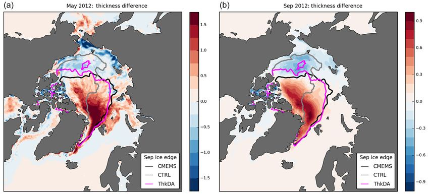
3420                      E. W. Blockley and K. A. Peterson: Improving Met Office seasonal predictions of Arctic sea ice

Arctic (Eicken, 2013). Improved knowledge of sea ice on            tion system (MacLachlan et al., 2014; Peterson et al., 2015),
seasonal timescales allows for better planning which should        which has contributed to the SIO since 2010. The ocean
lead to a reduced level of risk and a reduction in opera-          and sea-ice components of GloSea are initialized each day
tional costs for human activities in the Arctic Ocean. Re-         using the Forecast Ocean Assimilation Model (FOAM) op-
gional changes in Arctic sea-ice cover can also have implica-      erational ocean–sea-ice analysis of Blockley et al. (2014,
tions for lower latitude weather and climate (Koenigk et al.,      2015). FOAM routinely assimilates sea-ice concentration
2016; Balmaseda et al., 2010; Screen, 2013). For example,          (SIC) along with various ocean quantities – satellite and
Koenigk et al. (2016) show that late summer sea-ice cover          in situ sea surface temperature (SST), satellite sea level
can be linked to winter North Atlantic Oscillation (NAO)-like      anomaly (SLA), in situ profiles of temperature and salinity
patterns and blocking in Western Europe. Therefore, more           (T&S) – but, as is common with most operational ocean anal-
accurate Arctic sea-ice predictions can also contribute to im-     ysis systems (Tonani et al., 2015; Martin et al., 2015; Bal-
proved forecasts, and hence longer-term planning, in mid-          maseda et al., 2015; Cummings and Smedstad, 2014), does
latitude regions.                                                  not assimilate sea-ice thickness.
   Interest in seasonal predictions has increased following the       The use of dynamical models for seasonal sea-ice predic-
drastic reduction in Arctic sea-ice extent in the summer of        tion is in its relative infancy. Still, there have been several
2007, which led to a (then) record-low summer minimum              studies that demonstrate skill in retrospective forecasts (or
extent being set. In response to this, in 2008, the Sea Ice        hindcasts) of September-mean Arctic sea ice extent made
Outlook (SIO) was instigated by the Study of Environmen-           from spring (e.g. Sigmond et al., 2013; Wang et al., 2013;
tal Arctic Change (SEARCH) to synthesize seasonal pre-             Chevallier et al., 2013; Msadek et al., 2014; Peterson et al.,
dictions of September Arctic sea-ice extent, made from late        2015). However, none of these were able to match the poten-
spring and early summer, using a variety of modelling, sta-        tial skill found in idealized “perfect model” studies (Gue-
tistical, and heuristic approaches (see Stroeve et al., 2014).     mas et al., 2016; Tietsche et al., 2014; Day et al., 2014;
For seasonal forecasts to be of use to stakeholders, a thor-       Blanchard-Wrigglesworth et al., 2011), where all the ini-
ough understanding of their predictive skill is needed. The        tial conditions, but in particular, the sea-ice thickness, are
community that has been built up around the SIO has en-            known precisely. Furthermore, when applied to a real-time
abled collaborative activities addressing such issues across       forecast, as submitted to SIO, the skill was found to be even
various prediction centres through the inter-comparison and        lower than the hindcast skill (Blanchard-Wrigglesworth et
common evaluation of forecasts (see https://www.arcus.org/         al., 2015), and only marginally better than a linear trend fore-
sipn/sea-ice-outlook, last access: 4 October 2010). There is       cast (Stroeve et al., 2014). Clearly, there is potential for im-
also an interesting scientific problem here to test our ability    provement in the dynamical models if more complete initial
to predict sea ice on seasonal timescales that are considerably    conditions are known, with an even greater need, as demon-
longer than the (typically 1–2 week) limit, beyond which, the      strated by the deteriorated performance of the real-time fore-
chaotic nature of the atmosphere and ocean inhibit traditional     casts, for more accurate real-time initial conditions. None of
deterministic forecasting (Slingo and Palmer, 2011). As the        the systems mentioned above initialize the sea ice using ob-
sea ice thins, variability in ice extent increases (Holland et     served thickness measurements.
al., 2011; Goosse et al., 2009) and so the problem of mak-            Several studies have shown that winter sea-ice thickness
ing seasonal Arctic sea-ice predictions, particularly for the      provides important preconditioning for the evolution of Arc-
September minimum, is one that is getting more challenging         tic sea ice through the summer melt season. Blanchard-
and interesting as the ice cover declines (Holland et al., 2011;   Wrigglesworth and Bitz (2014) found sea-ice thickness
Stroeve et al., 2014).                                             anomalies in general circulation models (GCMs) to have a
   Although global coupled forecasting systems have been           timescale of between 6 and 20 months making their cor-
used successfully for seasonal prediction of mid-latitude          rect representation in model initial conditions of importance
weather and climate for some time now (see, for exam-              for seasonal predictions. Other modelling studies by Hol-
ple, Scaife et al., 2014), their application to Arctic sea-ice     land et al. (2011) and Kauker et al. (2009) have also shown
prediction is much less mature. In particular, forecasts in        that knowledge of winter ice thickness can provide some
the Arctic are hampered by the fact that observations are          predictive capability for summer ice extent. Perfect model
much less abundant and data assimilation techniques less           studies (e.g. Day et al., 2014) have also suggested that cor-
advanced in the polar regions than at lower latitudes (Jung        rect initialization of sea-ice thickness can lead to improved
et al., 2016; Bauer et al., 2016), meaning that the initial        seasonal forecasts. Day et al. (2014) used the HadGEM1.2
conditions used for forecasts in the Arctic are less accu-         climate model to show that memory of winter thickness
rate than for lower latitudes. Despite this, several opera-        conditions can persist well beyond seasonal timescales and
tional forecasting centres regularly contribute to the SIO with    provide predictive capability for up to 2 years. Collow et
sea-ice predictions from fully coupled atmosphere–sea-ice–         al. (2015) found considerable changes in ice concentration
ocean modelling systems. One such system is the Met Of-            forecasts when changing the initial thickness in the cou-
fice’s Global Seasonal (GloSea) coupled ensemble predic-           pled forecast system model version 2 (CFSv2) seasonal pre-

The Cryosphere, 12, 3419–3438, 2018                                                    www.the-cryosphere.net/12/3419/2018/
E. W. Blockley and K. A. Peterson: Improving Met Office seasonal predictions of Arctic sea ice                             3421

diction system. They showed an improvement to seasonal            late-summer (September) sea ice cover will be improved by
forecasts when using thickness fields from the Pan-Arctic         initializing sea ice thickness in early spring (May) using ob-
Ice–Ocean Model Assimilation System (PIOMAS) model of             servations of thick sea ice derived from CS2. In this study,
Zhang and Rothrock (2003). These studies suggest that sea-        we use a simple nudging technique to test this hypothesis,
sonal (> 90 days) predictions of Arctic summer sea ice, made      and evaluate the feasibility of including sea ice thickness
with dynamical models, could be improved by correctly ini-        initialization within the operational GloSea seasonal predic-
tializing sea-ice thickness. However, we note that, although      tion system. We assimilate CS2 sea ice thickness within the
uncertainty in the initial conditions plays a crucial role for    FOAM ocean–sea ice reanalysis and use these analyses as
seasonal predictions of Arctic sea ice, model uncertainty is      initial conditions for an ensemble of seasonal (5-month) cou-
likely to dominate the evolution of seasonal forecast errors      pled forecasts to determine the impact of sea ice thickness
(Blanchard-Wrigglesworth et al., 2017).                           initialization on the skill of GloSea seasonal predictions. We
   Although the assimilation of sea-ice concentration has         show that sea ice thickness initialization leads to a consider-
been included in ocean reanalysis, operational ocean predic-      able improvement in the skill of seasonal predictions of Arc-
tion and seasonal forecasting systems for several years (Stark    tic sea ice extent and ice edge location.
et al., 2008; Peterson et al., 2015), sea ice thickness is not       This paper is structured as follows: Sect. 2 introduces
yet routinely used to initialize these systems (Martin et al.,    the modelling systems and observations used in this study;
2015; Balmaseda et al., 2015; Tonani et al., 2015). However,      Sect. 3 describes the initialization of CS2 thickness within
there have been several recent studies that have sought to im-    the ocean–sea ice reanalysis and the generation of initial con-
prove the representation of Arctic sea-ice thickness in anal-     ditions for seasonal predictions; Sect. 4 provides details of
yses and short-range forecasts using satellite thickness prod-    GloSea coupled seasonal prediction experiments performed
ucts derived from Soil Moisture and Ocean Salinity (SMOS)         using CS2 initialized thickness and shows improved skill
brightness temperatures and/or from CryoSat-2 (hereafter          for seasonal forecasts of Arctic ice cover. Section 5 pro-
CS2) radar freeboard measurements. Such studies have gen-         vides summary discussion and an overview of proposed fu-
erally focused on assimilation of thickness using ensemble        ture work.
techniques into short-range, externally forced, ocean–sea-ice
models in the Topaz system (Xie et al., 2016) or using MIT-
gcm (Yang et al., 2014; Mu et al., 2018). Although these          2     Models and observations used in this study
studies showed considerable improvement to the simulation
of sea-ice thickness, the impact on short-range forecasts of      2.1    Modelling systems
sea-ice concentration or extent was minimal. More recently,
Allard et al. (2018) used direct initialization of CS2-derived    The model systems used in this study are taken from the
sea-ice thickness, using 2 different datasets processed with      Met Office suite of seamless, traceable prediction systems
different algorithms, within a series of reanalyses performed     introduced by Brown et al. (2012) using components of
with the Naval Research Laboratory’s forced ocean–sea ice         the Hadley Centre Global Environment Model version 3
Arctic Cap Nowcast/Forecast System (ACNFS). They show             (HadGEM3) coupled model architecture described by Hewitt
that the analysed sea ice thickness is significantly improved     et al. (2011). All of these HadGEM3-based modelling sys-
when assimilating CS2 thickness compared against in situ          tems simulate the ocean and sea ice conditions using the Nu-
and airborne measurements. They also perform an in-depth          cleus for European Modelling of the Ocean (NEMO) ocean
assessment of the thickness data and analyses, and show a         model (Madec, 2008) coupled to the Los Alamos sea ice
good agreement between the CS2-derived ice thickness and          model (CICE) (Hunke et al., 2015).
observations from in situ and airborne sources.                      Within the Met Office’s unified, seamless framework, sea-
   As noted above, several studies (Yang et al., 2014; Xie et     sonal forecasts are performed using the GloSea coupled pre-
al., 2016; Mu et al., 2018; Allard et al., 2018) have looked at   diction system (MacLachlan et al., 2014; Scaife et al., 2014).
the impact of sea ice thickness initialization on analyses and    GloSea produces two 210-day seasonal forecasts every day,
short-range forecasts produced with externally forced ocean–      which, together with those from previous days, are com-
sea ice models. What has not been investigated is the im-         bined to form a lagged ensemble prediction system. Mean-
pact that assimilation of sea ice thickness may have in longer    while hindcasts, retrospective forecasts performed for pre-
(> 90 days) forecasts made using fully coupled dynamical          vious years using true forecast conditions, are used to es-
models. Here we do so for the first time using the Met Of-        tablish errors in the model climatology for the purposes of
fice GloSea coupled seasonal prediction system. For accu-         bias correction, and to estimate forecast skill. More details
rate seasonal predictions of September sea ice cover, it is im-   on the GloSea seasonal prediction system can be found in
portant to model ice that will persist throughout the summer      MacLachlan et al. (2014). The ocean and sea ice components
season, and so an improved representation of the location         of the GloSea system are initialized each day using analyses
of thick sea ice within the initialization should be advanta-     from the FOAM system described in Blockley et al. (2014,
geous. We hypothesize that GloSea seasonal predictions of         2015). FOAM is an operational ocean–sea ice analysis and

www.the-cryosphere.net/12/3419/2018/                                                   The Cryosphere, 12, 3419–3438, 2018
3422                     E. W. Blockley and K. A. Peterson: Improving Met Office seasonal predictions of Arctic sea ice

forecast system run daily at the Met Office. Satellite and in    (Fetterer et al., 2016; Rayner et al., 2003), measurements of
situ observations of temperature, salinity, sea level anomaly    sea ice thickness are, relatively, much less abundant. How-
and sea ice concentration are assimilated by FOAM each           ever, satellite estimates of winter thickness have been avail-
day using the NEMOVAR 3D-Var First Guess at Appropri-            able for a number of years using radar altimetry (Laxon et al.,
ate Time (FGAT) scheme. Sea ice thickness is not currently       2003), laser altimetry (Kwok and Cunningham, 2008), and,
assimilated in FOAM; new ice is added by the concentration       more recently for thin ice, microwave brightness tempera-
assimilation at a default thickness of 0.5 m. More details of    tures (Kaleschke et al., 2016). Although radar altimeter esti-
the FOAM system can be found in Blockley et al. (2014)           mates of sea ice thickness have been available for many years
and more about the NEMOVAR 3D-Var FGAT scheme used               now, their up-take into operational ocean–sea ice assimila-
therein can be found in Waters et al. (2015).                    tion systems has been minimal. The primary reasons for this
   As well as the abovementioned operational analyses and        are 3-fold: the data were not made available in near-real-time
forecasts, longer reanalyses are performed with the FOAM         for use in operational analysis systems; owing to the orbit
system using surface forcing derived from the ERA-Interim        inclination, these datasets often have a large “pole hole” giv-
atmospheric reanalysis (Dee et al., 2011). Within the GloSea     ing poor coverage in the central Arctic Ocean; there is con-
seasonal prediction system, hindcast experiments initialized     siderable uncertainty associated with these estimates of ice
from these reanalyses are used to bias correct the GloSea        thickness (Ricker et al., 2014). The problems outlined above
seasonal forecasts (see MacLachlan et al., 2014, for more        have been ameliorated somewhat during the last few years by
information). As well as being used for bias correction          the launch of ESA’s CryoSat-2 satellite (CS2), the primary
within GloSea, these ocean reanalyses are utilized more          objective of which is to acquire accurate measurements of
widely within the ocean community (Balmaseda et al., 2015;       sea ice thickness. CS2 has an unusually high inclination or-
Chevallier et al., 2017; Uotila et al., 2018) and have been      bit that provides observational coverage up to 88◦ N, which
used to help answer a number of other scientific questions       has considerably reduced the size of the pole hole (Laxon et
(e.g. by Roberts et al., 2013; Jackson et al., 2015).            al., 2013). CS2 is also fitted with a Synthetic Aperture In-
   Throughout this study we shall use prototype FOAM and         terferometric Radar Altimeter (SIRAL) instrument that has
GloSea systems based on the latest configuration of the          a higher accuracy, and along-track resolution, than was pre-
Met Office coupled modelling system (GC3: Williams et            viously available from the ENVISAT and ERS-1/2 radar al-
al., 2017), which will be used as part of Met Office Hadley      timeters (Guerreiro et al., 2017). The processed data from
Centre’s contribution to phase 6 of the Coupled Model In-        CS2 is also provided in almost near-real-time by the Centre
tercomparison Project (CMIP6). This GC3 coupled model            for Polar Observation and Modelling (CPOM) (Tilling et al.,
version uses the GO6 ocean and GSI8 sea ice component            2016) making its use within operational analysis systems a
configurations described in Storkey et al. (2018) and Ridley     realistic proposition.
et al. (2018), respectively, and uses the extended ORCA025
tripolar grid described therein, with nominal 1/4◦ horizontal    2.2.1   CryoSat-2 thickness observations
resolution, ranging from 8.9 to 15.5 km in the Arctic Ocean
basin, and 75 vertical levels. The sea ice component of the      In this study, we initialize the model using thick ice from
model is based upon CICE vn5.1.2 and uses the standard           CS2, which are accurate for ice thicker than 1 m (Ricker
CICE elastic–viscous–plastic (EVP) rheology for modelling        et al., 2017). We use monthly CS2 winter (October–April)
the sea ice dynamics (Hunke et al., 2015). Growth and melt       thickness estimates produced by CPOM (Tilling et al., 2016),
of the sea ice is calculated using a multi-layer thermodynam-    which start from October 2010 until present (at time of writ-
ics scheme with 4 layers of ice and 1 layer of snow. At each     ing). Sea ice freeboard is inferred from radar altimetry aboard
model grid point, the sub-grid scale ice thickness distribu-     the CS2 satellite and is converted to thickness by assuming
tion is modelled by partitioning the ice into five thickness     that the sea ice floats in hydrostatic equilibrium and by mak-
categories (lower bounds: 0, 0.6, 1.4, 2.4, and 3.6 m), with     ing various assumptions about the snow loading and the rel-
an additional ice-free category for open water areas. The im-    ative densities of the sea ice, the ocean, and the overlying
pact of surface meltwater on the sea ice albedo is explicitly    snow. Details of the methods used to generate the CPOM
represented by the prognostic evolution of melt ponds using      thickness fields can be found in Laxon et al. (2013) and Till-
the topographic formulation. Further details about the sea ice   ing et al. (2015). Several different centres, including CPOM,
component, and the wider coupled model used here, can be         are now producing CS2-derived estimates of sea ice thick-
found in Ridley et al. (2018) and Williams et al. (2017), re-    ness. More details on the differences between these obser-
spectively.                                                      vational estimates can be found in Stroeve et al. (2018) and
                                                                 Allard et al. (2018). Some more general discussion of the
2.2    Observations of sea ice thickness                         uncertainties involved in the calculation of sea ice freeboard
                                                                 and thickness using radar altimetry can be found in Ricker et
Whilst observations of sea ice concentration providing large-    al. (2014).
scale coverage for both poles have been available since 1979

The Cryosphere, 12, 3419–3438, 2018                                                  www.the-cryosphere.net/12/3419/2018/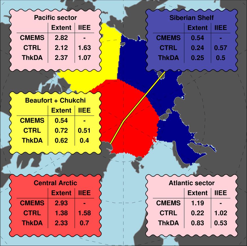
E. W. Blockley and K. A. Peterson: Improving Met Office seasonal predictions of Arctic sea ice                                 3423

   The CPOM thickness data are provided on a 5 km polar            described in http://marine.copernicus.eu/documents/QUID/
stereographic grid having been smoothed with an averaging          CMEMS-GLO-QUID-001-026.pdf, last access: 4 October
window of radius 25 km. We apply a further quality con-            2018). Using this CMEMS reanalysis has the benefit that it
trol (QC) to the data before use. The CS2 thickness retrieval      is performed on the same ORCA025 grid as the ocean–sea
methodology is particularly uncertain for thin ice where the       ice components of the GloSea seasonal forecasting system,
ice freeboard is not much higher than sea level (Ricker et         which makes spatial comparisons easier. This reanalysis has
al., 2014, 2017). To avoid high observational error associ-        also been evaluated thoroughly through the Ocean Reanal-
ated with these thin measurements we impose a minimum              yses Inter-comparison Project (ORA-IP) (see Balmaseda et
thickness threshold of 1 m, a choice that was motivated by         al., 2015; Chevallier et al., 2017; Uotila et al., 2018). To avoid
Fig. 2b of Ricker et al. (2017). Further, to ensure that the ob-   confusion with the FOAM reanalyses performed as part of
servations are as representative of the month as possible we       this study, and described later, we refer to this product as
apply the constraint that at least 10 different altimeter tracks   “CMEMS” hereafter.
are used to determine the monthly mean observation. We also
impose a constraint on the spread of the track observations by     2.3.2   Sea ice concentration datasets used for
keeping monthly observations only when the standard devi-                  assimilation
ation of the contributing individual track observations is less
than 2 m. Finally, we remove any spuriously high observa-          The CMEMS reanalysis, and the reanalyses performed in this
tions by imposing a maximum thickness threshold of 7 m. In         study, were performed using Special Sensor Microwave Im-
total, application of the abovementioned QC rejected roughly       ager/Sounder (SSMI/S) sea ice concentration data provided
21.5 % of the original observations; about 9.4 % of the obser-     by the European Organisation for the Exploitation of Meteo-
vations were removed by the 1m cut-off and just over 12 %          rological Satellites (EUMETSAT) Ocean and Sea Ice Satel-
were rejected by the remaining constraints. An example of          lite Application Facility (OSI-SAF). Sea ice concentration
the thickness observations used in this study can be seen in       is assimilated, together with ocean data sources using the
Fig. 1a, which shows a map of average October–April Arctic         NEMOVAR 3D-Var scheme (see Blockley et al., 2014; Wa-
thickness for 2011–2015 inferred from CS2 estimates after          ters et al., 2015). Prior to October 2009, OSI-SAF’s Global
application of the QC process described above.                     Sea Ice Concentration Climate Data Records (OSI-409, ver-
                                                                   sion 1.1) product was assimilated. When the reanalysis was
2.3     Observations of sea ice extent and concentration           run, in 2014, these data were only available up to the end
                                                                   of 2009 and so the OSI-SAF near-real-time (NRT) product
Within this study, observations of sea ice concentration and       OSI-401a was used from 25 October 2009 onwards. These
extent from several sources are used both for evaluating           two datasets have differences in the processing of low con-
seasonal predictions of Arctic sea ice, and for assimilation       centration ice and near coastlines (see Sect. 4.2 of OSI-SAF,
within the reanalyses used for initialization of these seasonal    2017). However, this does not cause us any concern here be-
predictions.                                                       cause our study is focused on the CS2 era from October 2010
                                                                   onwards.
2.3.1    Sea ice concentration and extent datasets used for
         evaluation                                                3   Initialization of thickness in the ocean–sea ice
                                                                       reanalysis system
Uncertainty associated with sea ice concentration and ex-
tent estimates from satellites is high (Ivanova et al., 2015)      Here we use the latest development version of the FOAM-
and the commonly used sea ice extent metric is non-                GloSea reanalysis system that has been undertaken as part of
linear and dependent on resolution (Notz, 2014). To ac-            the upgrade of GloSea and FOAM to use the latest GC3 ver-
count for this uncertainty we include observational estimates      sion of the Met Office coupled model architecture (Williams
from three different sources: extents calculated from the          et al., 2017). Specifically here the ocean reanalysis system
1◦ gridded Hadley Centre Sea Ice and Sea Surface Tem-              is using the GO6 ocean configuration described in Storkey
perature (HadISST1.2) dataset of Rayner et al. (2003); the         et al. (2018) and the GSI8 sea ice configuration described
National Snow and Ice Data Center (NSIDC) sea ice in-              in Ridley et al. (2018). We take the latest GO6+GSI8 re-
dex of Fetterer et al. (2016); and gridded sea ice concen-         analysis as our control (hereafter CTRL-RA) and modify it
tration fields from the most recent FOAM-GloSea ocean–             to include initialization of sea ice thickness using CS2 ob-
sea ice reanalysis. This reanalysis, performed using ver-          servations (hereafter ThkDA-RA). The CTRL-RA reanalysis
sion 13 of the FOAM system (Blockley et al., 2015), is             was run from 1992 to 2015 but here we only re-run the last
used within the Copernicus Marine Environment Moni-                5 years, from October 2010 to the end of 2015 , to tie in with
toring Service (CMEMS; http://marine.copernicus.eu/, last          availability of CS2 thickness estimates.
access: 4 October 2018) global ocean reanalyses ensem-
ble product (ID: GLOBAL-REANALYSIS-PHY-001-026;

www.the-cryosphere.net/12/3419/2018/                                                     The Cryosphere, 12, 3419–3438, 2018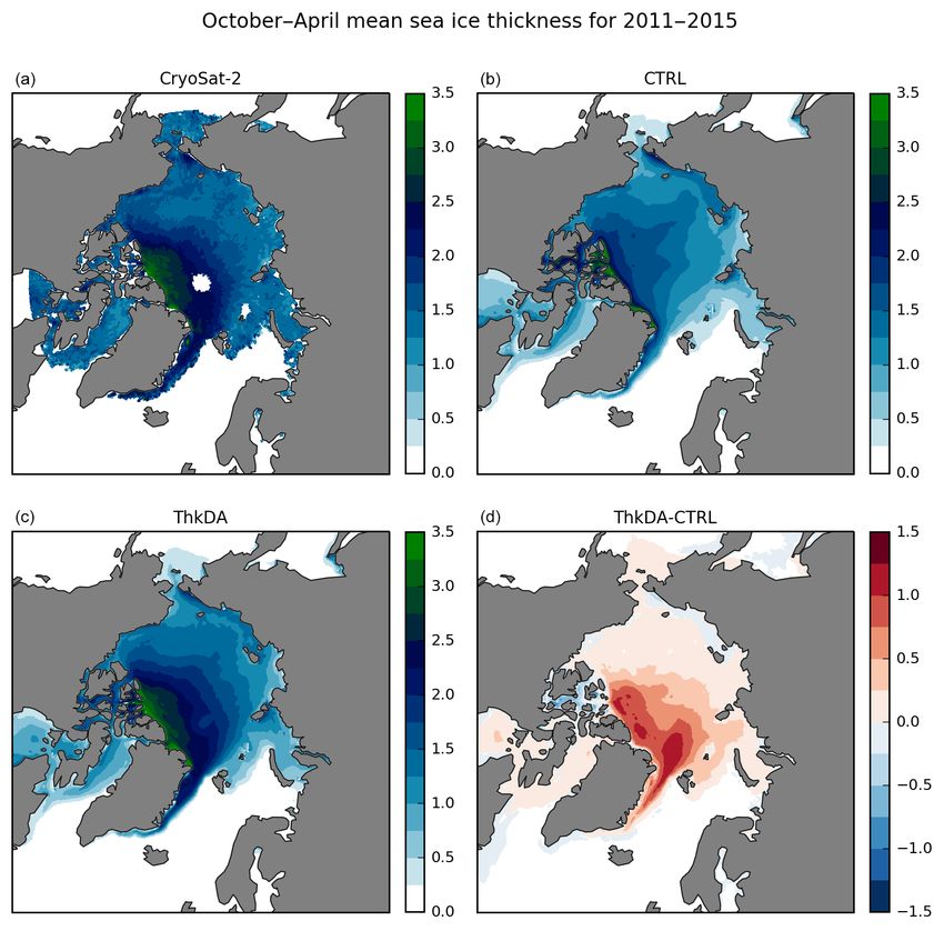
3424                        E. W. Blockley and K. A. Peterson: Improving Met Office seasonal predictions of Arctic sea ice

Table 1. Details of ocean–sea ice reanalysis experiments used in this study.

       Experiment name     Reanalysis run period        Surface forcing    Assimilated variables (3D-Var)   Thickness nudging used
       CTRL-RA             1 Jan 1992–31 Dec 2015       ERA-Interim        SST, SLA, T&S, SIC               None
       ThkDA-RA            1 Oct 2010–31 Dec 2015       ERA-Interim        SST, SLA, T&S, SIC               CPOM CryoSat-2

Figure 1. Mean winter (October to April) Arctic sea ice thickness (m) from October 2010 to April 2015 for (a) CPOM CryoSat-2 mea-
surements, after application of the QC and imposing the 1 m minimum thickness threshold; modelled thickness from (b) the CTRL and
(c) ThkDA reanalyses. Panel (d) shows the difference between the ThkDA and CTRL experiments.

   Within the ThkDA-RA reanalysis, CS2 thickness data are                 dard binning technique. A linear interpolation is performed
assimilated using a basic nudging technique in which thick-               each day to get daily thickness observations from the nearest
ness fields are nudged towards the monthly gridded CS2 ob-                two months. Assimilation increments are created by taking a
servations in a fashion akin to that employed by climato-                 simple difference between these daily CS2 thickness obser-
logical relaxation schemes. All other data used within the                vations and the daily mean model thickness. Where no obser-
control run (i.e. SST, SLA, T&S profiles, and SSMI/S sea-                 vations are present, the increments are set to zero to ensure
ice concentration) are assimilated here too in the same man-              no thickness nudging is performed. We do things this way to
ner as in the standard FOAM system (Blockley et al., 2014,                avoid problems arising with the sparse data and so we can
2015). The sea ice concentration observations assimilated are             keep nudging the model towards CS2 thickness.
the same as used for the CMEMS reanalysis described in                       The increments are applied within the CICE model code
Sect. 2.3.2 above (i.e. OSI-401a). An overview of reanaly-                in a similar fashion to the sea ice concentration assimila-
sis experiments used in this study can be found in Table 1.               tion described in Peterson et al. (2015) and Blockley et
   We use the monthly CPOM measurements introduced in                     al. (2014). Thickness changes are made at each time step
Sect. 2.2 and map them onto the model grid using a stan-                  using the Incremental Analysis Update (IAU) method. A 5-

The Cryosphere, 12, 3419–3438, 2018                                                          www.the-cryosphere.net/12/3419/2018/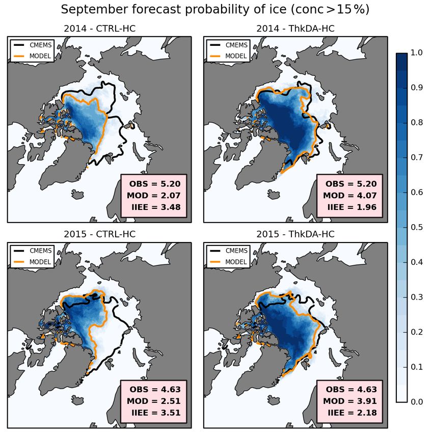
E. W. Blockley and K. A. Peterson: Improving Met Office seasonal predictions of Arctic sea ice                               3425

Figure 2. Reanalysis Arctic sea ice volume from 1 October 2010 to the end of December 2015 from the CTRL-RA (blue) and ThkDA-RA
(red) reanalysis experiments. Sea ice volume from the PIOMAS model (grey dashed) is included as a reference.

day relaxation timescale is used and increments are only ap-         creased the most by the assimilation of CS2 thickness. This
plied where the grid-cell ice concentration is above 40 %.           is perhaps not surprising given that winter is the time when
The CICE sea ice model uses multiple thickness categories            the data are available. However, there is some evidence that
to represent the sub-grid thickness distribution. To apply the       these winter changes also affect the summer volume, which
thickness increments into the multi-category model we chose          is most pronounced in 2014 and, to a lesser extent, 2013
to nudge the grid-box-mean thickness towards observations            and 2015. In all years, the volume time series shows a clear
by making changes across each of the 5 sub-grid categories,          kink on 1 October when the CS2 data comes back online
so long as there is ice present there with concentration above       and begins to be assimilated in the reanalysis, although this
1 %, maintaining the initial distribution of volume between          is much less pronounced in 2014 when the summer thick-
the categories. We note here that this approach is similar           ness was also increased. In Fig. 2, sea ice volume for the
to that employed by Allard et al. (2018), who multiply the           CTRL-RA and ThkDA-RA reanalyses are also compared
ice volume in each category by the grid-box-mean model-              with volume estimates from the PIOMAS model of Zhang
observation thickness difference. However, whilst they use           and Rothrock (2003). The PIOMAS volume is included here
direct initialization, we use the IAU approach to incorporate        purely as a reference because it is well understood and widely
changes into the model in a gradual manner and limit the po-         used for this purpose. The volume in the CTRL-RA run is
tential for sudden shock in the system (Bloom et al., 1996).         much closer to PIOMAS than the ThkDA-RA run. This is ex-
                                                                     pected as PIOMAS has been shown to underestimate thick-
3.1   Impact of CryoSat-2 initialization on reanalysis               ness and volume in the winter compared to the CPOM CS2-
      thickness                                                      derived thickness (Tilling et al., 2015; Laxon et al., 2013),
                                                                     although it has been shown to compare better with laser al-
Figure 1 illustrates the general impact of including CS2 as-         timeter estimates such as ICESat (Schweiger et al., 2011).
similation within the ThkDA-RA reanalysis by showing the                Figure 3a shows the impact of the CS2 thickness initializa-
mean Arctic sea ice thickness for the months when CS2 data           tion on the reanalysis end of winter thickness fields, which
are available (October–April) over the whole ThkDA-RA re-            will be used in this study to initialize GloSea seasonal pre-
analysis (2010–2015). The difference plot in Fig. 1d shows           dictions, with the 5-year mean differences for 1 May at the
that the inclusion of CS2 nudging generally acts to increase         end of winter when CS2 observations cease. At the end of
the thickness of the Arctic sea ice, in particular in the Atlantic   winter it is apparent that inclusion of CS2 thickness nudg-
sector north of Fram Strait, and to the north of Greenland.          ing has increased sea ice thickness across much of the At-
Comparison with the observations in Fig. 1a shows that the           lantic sector of the Arctic (Barents, Kara and Greenland
thickness in ThkDA-RA is much more closely aligned with              Seas). Conversely, ice thickness has been decreased in the
the CS2 data than is the case for CTRL-RA.                           Canadian Arctic Archipelago (CAA) and, to a lesser degree,
   A comparison of sea ice volume for the CTRL-RA and                across much of the Pacific sector (Beaufort, Chukchi and
ThkDA-RA reanalyses in Fig. 2 confirms that the net effect           East Siberian Seas). Thickness is also increased in many of
of CS2 thickness nudging is an increase in sea ice thickness.        the marginal seas outside of the central Arctic such as the
We note that an increase in volume here directly implies an          Bering Sea and Hudson Bay. One notable exception is the
increase in average ice thickness because, as sea ice con-           Labrador Sea and Baffin Bay where the differences form an
centration is tightly constrained by the assimilation of sea         east–west dipole with ice thickness being reduced along the
ice concentration and sea surface temperature, the ice area          Canadian coast but increased on the Greenland side.
between the two reanalysis simulations is virtually identi-             Figure 3b shows the 5-year-mean difference in the reanal-
cal (not shown). Figure 2 shows that winter volume is in-            yses thickness fields at the end of summer (30 September) af-

www.the-cryosphere.net/12/3419/2018/                                                      The Cryosphere, 12, 3419–3438, 2018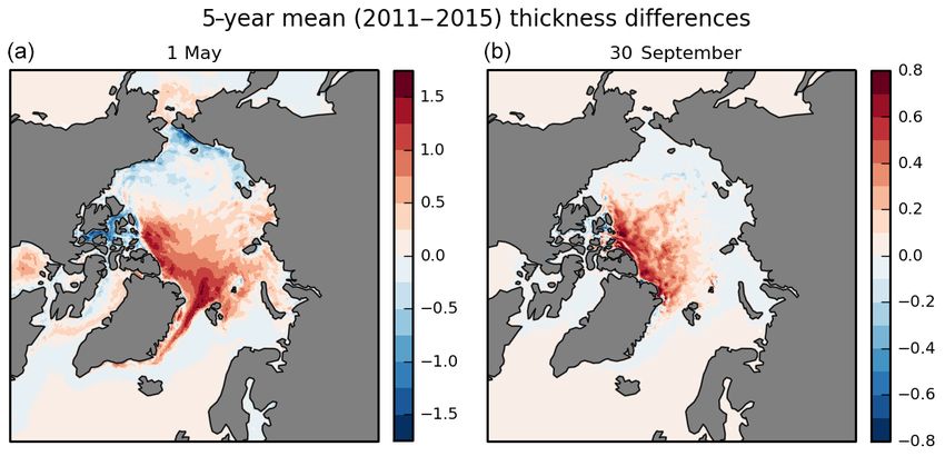
3426                        E. W. Blockley and K. A. Peterson: Improving Met Office seasonal predictions of Arctic sea ice

Figure 3. Mean sea ice thickness difference (m) between ThkDA-RA and CTRL-RA experiments over the full 5-year reanalysis period from
2011 to 2015. Showing differences for (a) the end of winter on 1 May used for the initialization of summer seasonal forecasts, and for (b) the
end of summer on 30 September. The difference is taken as ThkDA–CTRL so red and blue imply that the CS2 nudging have increased and
decreased the thickness, respectively.

ter 5 months of running without thickness assimilation. The                 In summary, we have shown that nudging Arctic sea ice
impact of the CS2 nudging is an increase in sea ice thick-               thickness to CS2 observations within the ThkDA-RA reanal-
ness throughout much of the Arctic save for small patches                ysis has the net effect of increasing sea ice volume. The dif-
in the East Siberian Sea and within the CAA. The pattern                 ferences between the two reanalyses reveal a persistent bias
is broadly consistent with the differences seen at the end of            in the thickness distribution in the model when compared
winter in Fig. 3a. Even after 5 months of running without the            with CS2, whereby sea ice is too thick on the Pacific side and
CS2 thickness nudging, although still assimilating ice con-              not thick enough on the Atlantic side of the Arctic. There is
centration and other ocean quantities, we can see the impact             evidence to suggest that the winter Arctic sea ice thickness
of initializing thickness through the winter. This is good news          and volume is an important precondition for evolution of ice
for the feasibility study because it tells us that the thickness         through the melt season (in agreement with the current litera-
changes are being retained by the model and not being re-                ture) because the effects of winter thickness changes imposed
jected or washed out by the assimilation of other quantities             by the nudging are still evident at the end of the summer. An-
such as ice concentration.                                               other important result to note here is that the assimilation of
   The general picture shown by the 5-year mean in Fig. 3a               thickness worked well and the increments were successfully
is typical of the end of winter thickness differences seen for           retained by the model, which bodes well for inclusion of sea
each of the 5 years 2011–2015 (not shown). Mean sea ice                  ice thickness within the NEMOVAR system in the future.
thickness across the Arctic Ocean basin has been increased
by around 14 % (from 2.00 to 2.27 m). This increase is most
pronounced in the Atlantic sector of the Arctic (30◦ W–                  4    Initialization of thickness in the GloSea coupled
140◦ E), where thickness increased by around 33 % (from                       seasonal prediction system
1.44 to 1.91 m). Although mean thickness in the combined
Beaufort and Chukchi Seas has decreased by 7 % (from 2.32                Seasonal forecasts of sea ice extent are made operationally
to 2.15 m), the net effect over the whole Pacific sector of the          by the GloSea system each day. Hindcast predictions, per-
Arctic (140◦ E–20◦ W) is an increase of 6.6 % (from 2.33                 formed from a discrete predefined set of start dates each year,
to 2.49 m). However, the situation is not so clear-cut for the           are also run within the operational suite each day and used
summer case (Fig. 3b), where thickness increases are much                as part of the bias correction process. These hindcast pre-
more pronounced in 2014 and 2013 (see Fig. 2).                           dictions are initialized using the long GloSea ocean–sea ice
   The impact of the thickness changes on the large-scale                reanalysis (as described in Sect. 3), which is coupled to atmo-
sea ice motion is negligible with monthly mean velocities in             sphere initial conditions interpolated from the ERA-I reanal-
the two experiments being virtually identical throughout the             ysis (Dee et al., 2011). In addition to being used operationally
2011–2015 period (not shown). This is consistent with the                for bias correcting forecasts, seasonal hindcasts such as this
findings of Allard et al. (2018), who show little impact on ice          are performed for testing of model configuration upgrades
drift in their reanalysis comparisons.                                   prior to implementation within the GloSea operational suite.
                                                                         As these hindcasts are used to test the expected skill of a real
                                                                         forecast, they are performed in a fashion that does not use any

The Cryosphere, 12, 3419–3438, 2018                                                            www.the-cryosphere.net/12/3419/2018/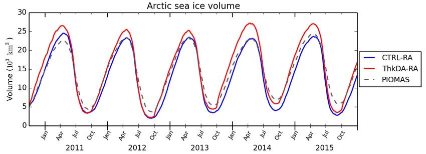
E. W. Blockley and K. A. Peterson: Improving Met Office seasonal predictions of Arctic sea ice 3427
Table 2. Details of GloSea coupled seasonal prediction experiments (or “hindcasts”) used in this study.
Experiment name Prediction lead time Years Ensemble members Atmosphere ICs Ocean–ice ICs
CTRL-HC May–Sep 1992–2015 24 per year∗ ERA-Interim CTRL-RA
ThkDA-HC May–Sep 2011–2015 24 per year∗ ERA-Interim ThkDA-RA
FIXED-IC May–Sep 2011–2014 24 per year∗ ERA-Interim ThkDA-RA:
fixed 2015 for all years
∗ 24 members per year = 3 start dates with 8 stochastic members for each.
subsequent observational data after initialization, so as not ble run with initialized thickness (ThkDA-HC; pink). Predic-
to invalidate that expectation. A recent trial of the new GC3 tions from each of the 24 ensemble members, initialized from
coupled model configuration of Williams et al. (2017) has the 3 April or May start-dates, are depicted by the crosses;
been performed using the GloSea seasonal prediction sys- the ensemble mean is plotted with bold symbols and inter-
tem, which we shall use as our control (denoted CTRL-HC). connecting lines. Although the ThkDA-HC predictions only
The ocean and sea ice for these hindcasts are initialized us- start from 2011 we plot the CTRL-HC throughout the whole
ing the control reanalysis (CTRL-RA) described in Sect. 3 period of the run from 1992 to 2015 to help put the, relatively
and the atmosphere is initialized from the ERA-I reanalysis. short, 5-year time series into context. To assess the accuracy
As the GC3 developments include the implementation of a of the GloSea seasonal predictions, observational and reanal-
new multi-layer model for terrestrial snow (see Walters et al., ysis estimates of Arctic extent, from the CMEMS reanalysis,
2017; Williams et al., 2017), the snow fields were initialized and the HadISST and NSIDC datasets (see Sect. 2.3), are
separately from the atmosphere using a standalone version plotted alongside the model predictions (black or grey). We
of the GC3 land surface component (Joint UK Land Envi- note here that the difference in extent prior to 2010 between
ronment Simulator; JULES) with ERA-I snow precipitation the CMEMS reanalysis and the HadISST and NSIDC data
and data assimilation. sources apparent in Fig. 4a is caused by the switch in OSI-
Here we wish to test the impact of initializing with CS2 SAF data products in October 2009, from OSI-409 version
sea ice thickness on the seasonal predictions of September 1.1 to OSI-401a, described in Sect. 2.3 above. Being prior
sea ice extent. For this purpose, an ensemble of seasonal to the launch of CS2, this change does not have any impact
prediction experiments was configured that was identical to on the results of our study but we include all years avail-
the CTRL-HC experiment except that the ocean and sea ice able from CTRL-HC in Fig. 4 to build a picture of the skill
components were initialized from the ThkDA-RA reanal- of the CTRL-HC predictions made without sea ice thickness
ysis instead of CTRL-RA. Seasonal predictions were per- initialization. Figure 4 illustrates that, throughout the CTRL-
formed from 3 different spring start dates (25 April, 1 May HC experiment, the seasonal predictions of sea ice extent are
and 9 May). For each of these start dates, an ensemble of 8 consistently biased low. The mean extent over the full time
seasonal predictions was initialized from the same analysis series (1992–2015) of 4.20 × 10⁶ km2 is between 1.53 and
fields with spread between the members achieved by using 2.21 × 10⁶ km2 below that for the 3 observational datasets.
stochastic physics (see MacLachlan et al., 2014, for more de- The total extent comparisons in Fig. 4a show that the run
tails). This methodology is identical to that used for CTRL- with initialized winter thickness gives improved predictions
HC and, through a mixture of lagged and perturbed methods, of September sea ice extent. This is particularly true for
provides an ensemble of 24 forecasts of September sea ice 2011 and 2012, for which the ThkDA-HC predictions of to-
each year. These predictions were performed for 2011–2015, tal extent are within 0.12 × 10⁶ km2 of the observed values.
each year that spring analyses are available from the ThkDA- The underestimation of basin-wide extent seen throughout
RA ocean reanalysis. We denote this system of predictions as the CTRL-HC predictions has been reduced; 2011–2015 5-
ThkDA-HC. Details of the GloSea coupled prediction exper- year-mean extent of 3.78 × 10⁶ km2 for ThkDA-HC is much
iments used in this study can be found in Table 2. closer to the observational average of 4.62×10⁶ km2 than the
CTRL-HC value of 2.79 × 10⁶ km2 (Fig. 4a) is to the same
4.1 Improvements to seasonal prediction of Arctic observations.
extent and ice edge location Basin-wide extent is not a very useful metric for assessing
sea ice because, although it provides information about the
amount of ice present, it does not take into account the lo-
Results from the ThkDA-HC experiment show that the CS2
cation of the ice or the position of the ice edge – which are
thickness initialization has considerably improved the skill
more useful for operational users (Notz, 2014). To assess the
of GloSea seasonal predictions of Arctic sea ice cover. Fig-
skill of GloSea seasonal predictions in relation to the spa-
ure 4a shows September-mean Arctic sea ice extent from the
tial distribution of ice and ice edge location, we use the inte-
GloSea control ensemble (CTRL-HC; blue) and the ensem-
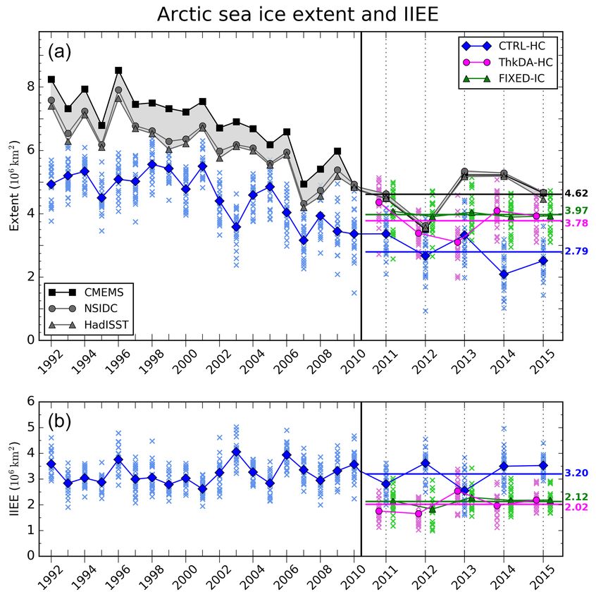
www.the-cryosphere.net/12/3419/2018/ The Cryosphere, 12, 3419–3438, 20183428 E. W. Blockley and K. A. Peterson: Improving Met Office seasonal predictions of Arctic sea ice Figure 4. (a) September-mean Arctic sea ice extent from the CTRL-HC (blue), ThkDA-HC (pink), and FIXED-IC (green) seasonal pre- diction experiments. Observational estimates from the CMEMS reanalysis assimilating OSI-SAF (black squares), NSIDC (grey circles) and HadISST1.2 (grey triangles) are included and the area between them shaded light grey. (b) Integrated ice edge error (IIEE) for seasonal predictions relative to the CMEMS reanalysis product introduced in Sect. 2.3. In both panels, individual ensemble members are represented by coloured crosses and ensemble means by the solid symbols and inter-connecting lines. Horizontal coloured lines depict 2011–2015 mean values. For ease of viewing, the ThkDA-HC (pink) and FIXED-IC (green) experiments are plotted with a small offset relative to the CTRL- HC (blue) experiment, and the CS2 period (2011–2015) is plotted with an increased x axis scale, approximately twice that for the early period 1992–2010, with the transition indicated by a vertical black line. grated ice edge error (IIEE) metric introduced by Goessling length of the full time series (1992–2015) illustrating that, as et al. (2016). This metric is essentially the area integral of for extent, the model without sea ice thickness assimilation all model grid cells where the forecast and observations dis- is consistently biased throughout this 24-year period. agree about whether sea ice is present or not (see Goessling Figure 4b shows that ice-edge error is considerably im- et al., 2016, for more details). Here we use a sea ice concen- proved by the CS2 thickness initialization with the 2011– tration threshold of 15 % to define whether ice is present or 2015 mean IIEE reduced from 3.20×10⁶ km2 for CTRL-HC not in any particular grid cell and compare the GloSea sea- to 2.02 × 10⁶ km2 for ThkDA-HC, a reduction of 37 %. The sonal predictions to the CMEMS reanalysis that assimilated differences in both extent and IIEE shown in Fig. 4 are sig- the OSI-SAF data. The GloSea and CMEMS products are nificant at the 1 % level over the whole 5-year period and for on the same ORCA025 grid and so comparisons between the each of the individual years, except for 2013. In general, the two are easy and not degraded by having to remap the data improvement in the ice edge location and IIEE is more pro- between different grids. Results from the IIEE analysis can nounced than the improvement to the basin-wide extent. This be found in Fig. 4b, which shows IIEE for each ensemble is to be expected given that the CS2 thickness initialization member of the CTRL-HC and ThkDA-HC GloSea seasonal changed the distribution of sea ice thickness in the Arctic as predictions (as in Fig. 4a, but for IIEE not extent). For the well as increasing average thickness. Figure 5 further illus- CTRL-HC experiment, the IIEE is virtually flat across the trates the spatial improvement in sea ice predictions showing The Cryosphere, 12, 3419–3438, 2018 www.the-cryosphere.net/12/3419/2018/
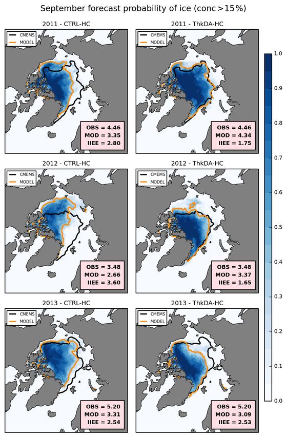
E. W. Blockley and K. A. Peterson: Improving Met Office seasonal predictions of Arctic sea ice                            3429

Figure 5.

the probability of ice across the CTRL-HC and ThkDA-HC          HC. In particular, the ThkDA-HC ensemble-mean ice edges
ensembles for each year (2011–2015), with ensemble-mean         for 2011 and 2012 are very close to those produced by the
and observed ice extent (represented by 15 % concentration      CMEMS reanalysis. A consistent feature of Fig. 5 is that
contours) overlain. Here we calculate the probability of ice,   the ice edge along the Atlantic sector of the Arctic is very
at each grid-cell, as the proportion of ensemble members for    well defined for the ThkDA predictions and is very close to
which the ice concentration is at least 15 %. Consistent with   the CMEMS reanalysis for all years. These improvements
the IIEE results in Fig. 4b, the ice edge location in Fig. 5    are further illustrated in Fig. 6, which shows, for several dif-
for the ThkDA-HC system is much better than for CTRL-           ferent Arctic Ocean regions, the ice extent predicted by the

www.the-cryosphere.net/12/3419/2018/                                                 The Cryosphere, 12, 3419–3438, 2018
3430                       E. W. Blockley and K. A. Peterson: Improving Met Office seasonal predictions of Arctic sea ice

Figure 5. September mean probability of sea ice for the CTRL-HC (left) and ThkDA-HC (right) seasonal predictions for all years from
2011 (top) to 2015 (bottom). Contours of 15 % concentration are overlain to represent the sea ice edge for the ensemble mean (orange) and
CMEMS reanalysis product (black). Probability is defined at each point as the proportion of ensemble members that have at least 15 % ice
concentration. The CMEMS extent, modelled extent and corresponding Integrated Ice Edge Error (IIEE) are included, for each plot, in the
lower-right corner (units: 106 km2 ).

CTRL and ThkDA experiments, along with the extent from                 experiments, for both the analysed spring initial conditions
the CMEMS reanalysis and the corresponding IIEE. The pre-              and the September-mean seasonal predictions, relate to the
dictions made using CS2 initialization (ThkDA) have lower              eventual predictions of ice edge. The thickness dipole from
extent in the Beaufort and Chukchi Seas and higher extent ev-          the CS2 nudging matches up well with the areas of miss-
erywhere else. In all regions, the ThkDA extent predictions            ing ice in the Atlantic sector and the areas of excess ice in
are closer to the CMEMS reanalysis and the corresponding               the Beaufort Sea. This suggests a strong relationship, in this
IIEE is lower. Improvements are most notable in the central            model at least, between wintertime thickness biases and the
Arctic region, and particularly the Atlantic sector.                   evolution of errors in sea ice concentration through the sum-
   The spatial changes in the September-mean sea ice con-              mer.
centration predictions depicted in Fig. 5 match well with the
May mean thickness dipole shown in Fig. 3a. A good illustra-           4.2   Wider impact of Arctic sea ice changes
tion of this is 2012 for which the extent improvement is much
smaller than the IIEE improvement (Fig. 4), which is caused            We now consider how the abovementioned sea ice improve-
by the fact that much of the ice that remains in the CTRL-             ments affect the wider GloSea seasonal September predic-
HC predictions is located in the Beaufort Sea rather than in           tions. With the changes in winter ice thickness, and in the
the Atlantic sector (north of Fram Strait/Svalbard and east of         evolution of Arctic ice coverage through the melt season de-
Greenland). Figure 7 further illustrates this point by showing         scribed above, one would expect to see both fast changes
how thickness differences between the CTRL and ThkDA                   to the local Arctic surface boundary layer (Semmler et al.,
                                                                       2016), as well as longer timescale changes to the wider atmo-

The Cryosphere, 12, 3419–3438, 2018                                                         www.the-cryosphere.net/12/3419/2018/
E. W. Blockley and K. A. Peterson: Improving Met Office seasonal predictions of Arctic sea ice 3431
same distribution. The resulting error difference fields cal-
culated using this method are qualitatively the same as con-
sidering the difference between the RMSE of each ensemble
mean relative to ERA-I (not shown); however, the errors here
will be larger as there will be no cancellation of errors caused
by averaging across ensemble members
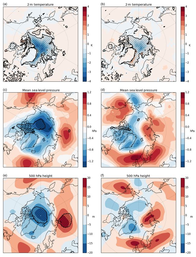
We first focus on the local temperature changes, for which
Fig. 8 shows that, owing to the overall increase in Arctic sea
ice thickness and extent, the ThkDA predictions show a gen-
eral cooling of September T2M, which is significant at the
95 % level over most of the Arctic Ocean. This cooling im-
proves the model error relative to the ERA-I atmospheric re-
analysis over the majority of this area (Fig. 8). The exception
to this is south of the Fram Strait in ice export regions, where
the T2M has become too cool. We hypothesize that this small
increase in error is likely due to the model simulating too
much sea ice transport south through the Fram Strait. Inter-
estingly, this improvement is also seen over perennially ice
Figure 6. Mean September Arctic sea ice extent for 2011–2015
from the CMEMS reanalysis (using OSI-SAF) compared with mod-
covered regions north of Greenland and the Canadian Arc-
elled extent and ice edge error (IIEE) from the CTRL and ThkDA tic Archipelago, where significant improvements in air–sea
seasonal predictions (units: 106 km2 ). Data are shown for 3 re- fluxes would not necessarily be expected. On the Pacific side
gions distinguished by the underlying shading and corresponding of the Arctic Ocean, where T2M in the ThkDA experiment is
box colours: combined Beaufort and Chukchi Seas (yellow), com- higher than for the CTRL experiments, very little improve-
bined Kara, Laptev and East Siberian Seas (Siberian Shelf; dark ment (or degradation) of the T2M is seen.
blue) and the central Arctic (red). Also shown (pink boxes) are cor- We next consider the longer timescale quasi-equilibrium
responding statistics for the Atlantic and Pacific sectors of the Arc- response (Semmler et al., 2016) to the pressure fields (MSLP
tic Ocean, defined by splitting the Arctic Ocean (i.e., the combined and z500). A significant decrease in MSLP and z500 is seen
red, yellow and dark blue areas) along 30◦ W and 140◦ E longitude in the ThkDA experiment over the Arctic Ocean with an
(yellow lines), which roughly follows the Lomonosov Ridge.
accompanying increase over Siberia (for z500, significantly
so), and with small non-significant increases over the North
Atlantic and Pacific (Fig. 8). This reduction leads to a de-
spheric circulation. While much of the recent work on large- crease in error over the Canadian Basin and Greenland, but
scale circulation has focused on changes to winter circulation slightly worse comparison with observations over the Bar-
(Koenigk et al., 2016; Vihma, 2014), studies have shown in- ents Sea and Western Europe. However, these differences
creased Northern European summer (Screen, 2013; Wu et al., in error are generally not significant save for a small patch
2013) and East Asian summer monsoon precipitation (Guo et of improved MSLP over the Canadian Arctic Archipelago
al., 2014) in association with reduced sea ice. (Fig. 8).
Figure 8 shows the difference between the ThkDA and The z500 and MSLP decrease over the Arctic is sugges-
CTRL predictions of September-mean near-surface air tem- tive of an increase in both the Arctic Oscillation (AO) and
perature (T2M), mean sea level pressure (MSLP), and NAO indices. This is consistent with other studies that have
500 hPa geopotential height (z500). Panels (a), (c), and (e) linked lower Arctic sea ice coverage with a tendency for a
show the mean difference, over all ensemble members and more meridional atmospheric jet (Francis and Vavrus, 2012),
all years (2011–2015), between the ThkDA predictions and along with a tendency toward the negative phase of the NAO
the CTRL predictions. Meanwhile panels (b), (d), and (f) (Petoukhov and Semenov, 2010). It is also broadly consistent
show the mean difference in root-mean-square-error (RMSE) with the lower Arctic z500 and wave-train nature of pressure
between the ThkDA predictions and the CTRL predictions. anomalies over Eurasia observed in Wu and Zhang (2013)
Here RMSE is calculated for each ensemble member relative and Screen et al. (2013) for summertime circulation patterns
to the ERA-I atmospheric reanalysis, which are then aver- related to above average sea ice areal coverage. However,
aged over all ensemble members and all years (2011–2015) owing to the small sample of years looked at here, it is doubt-
before differencing. Defining the error with respect to indi- ful we could establish a link with increased predictive skill of
vidual ensemble members in this manner, as opposed to look- the inter-annual variability of the atmospheric mid-latitude
ing at the ensemble mean error, provides a sufficiently large circulation.
distribution of values to allow us to test statistical signifi-
cance, which we do using a Mann–Whitney test with the null
hypothesis that all errors (or differences) are drawn from the
www.the-cryosphere.net/12/3419/2018/ The Cryosphere, 12, 3419–3438, 2018You can also read