APPENDIX B: GLOBAL AND REGIONAL SEA LEVEL RISE: A REVIEW OF THE SCIENCE

APPENDIX B: GLOBAL AND
REGIONAL SEA LEVEL RISE:
A REVIEW OF THE SCIENCE
Sea level rise is increasingly being considered in coastal planning. Decision-makers require robust projections of future
sea level in order to make informed decisions regarding coastal planning and adaptation. Of particular importance are
the upper limit or ‘worst-case scenario’ projections, which are low probability, high impact events. Underestimates of
sea level rise will leave coastal communities and infrastructure vulnerable to potential impacts, while overestimates of
sea level rise will result in unnecessary investments in coastal preparedness. This means it is particularly important to
understand the sources of uncertainty in sea level rise projections. The purpose of this appendix is to provide a readable
summary of the science of sea level rise and some justification for selecting the Kopp et al. (2014) approach that is used
in the main body of this report.

Climate change projections beyond 2100 are relatively limited. As a result, the majority of studies focus on end-of-
century global or regional sea level projections. We adopt the same convention for the current review. It is worth
emphasizing that this choice is arbitrary: the effects of climate on ice sheets and the ocean will continue well beyond
2100, and most studies indicate a continued rise in sea level after that time (Church et al., 2013a).

GLOBAL SEA LEVEL RISE PROJECTIONS
Overview: Process-based, Semi-Empirical Models,
and Expert Elicitation
There are several different approaches for projecting changes in global mean sea level. Process-based models and semi-
empirical models (SEMs) are two of the most frequently used approaches for projecting global sea level rise (SLR). Often
described as the “conventional” approach, process-based models rely on numerical modelling to simulate changes in,
and then sum the individual contributions of sea level rise components: thermal expansion, land-based glaciers, water
storage (reservoirs) and extraction (groundwater pumping), and the Greenland and Antarctic ice sheets.

Process-based models are currently unable to capture some key mechanisms which drive GMSL. Despite improvements
over the process-based models used in the Intergovernmental Panel on Climate Change’s (IPCC) fourth assessment
report (AR4; IPCC 2007), the process-based models used in the fifth assessment report (AR5; Church et al., 2013a) are
still limited in their ability to capture ice-sheet dynamical changes for each greenhouse gas scenario. The IPCC
assessment reports use process-based projections for GMSL. More information on the IPCC and the assessment reports
is provided in the call-out box on “The IPCC, GCMs, GHG Scenarios, Likelihood Terminology.”

Appendix B: Global and Regional Sea Level Rise: A Review of the Science Page 1 of 46

SEMs, in contrast, do not separate out individual components of sea level rise. Instead, these models derive statistical
relationships between sea level and temperature or radiative forcing from the observed historical record (i.e., from a
small network of long tide-gauge records) or longer proxy records1. SEMs make the assumption that the historically
derived relationship between temperature and sea level will continue, unchanged, into the future. This assumption may
fail to capture potentially nonlinear processes that may result in rapid glacier melt or alter the efficiency of ocean heat
uptake. The IPCC’s AR5 notes that because of this “...there is low agreement and no consensus in the scientific
community about the reliability of SEM projections, despite their successful calibration and evaluation against the
observed 20th century sea level record (Church et al., 2013a).”

Despite advancements in SEMs and process-based models, both approaches are currently limited in their ability to
capture the contribution of rapid ice sheet dynamics (e.g., calving) to sea level. As a result, expert elicitations have been
used to characterize uncertainty surrounding GMSL projections. Expert elicitations are used in many different fields
ranging from medicine to natural science, and can be useful when data or models are unable to adequately capture
physical processes or thresholds (Bamber & Aspinall, 2013). Expert elicitations can be divided into two general
categories: “broad” and “deep” elicitations (Horton et al., 2014). Broad elicitations administer short surveys to a large
number of experts, while, deep elicitations administer in-depth surveys to a smaller pool of experts. Recently, expert
elicitations have been used as a tool for assessing expert scientific opinion and quantifying the level of certainty on ice
sheet contribution to future global sea level (Bamber & Aspinall, 2013). Results of expert elicitations related to sea level
rise are discussed in greater detail in the “Upper Limits of Sea Level Rise” section.

Finally, it should be noted that this overview has focused on approaches to estimating global mean sea level rise
resulting from all contributions to sea level. In practice, a combination of process-based, empirical, and expert elicitation
is often used to produce estimates of the individual components of sea level rise.

Individual Sea Level Rise Components
Long-term average sea level change can be divided into four contributing components:

 1) Thermal expansion,

 2) Land-based glaciers and ice caps,

 3) The Greenland ice sheet (GIS) and Antarctic ice sheet (AIS), and

 4) Land water storage.

1 Proxy records or data are frequently used when studying historical climate conditions. Proxy records are preserved physical or natural
 conditions which can be used today to find out more about what climate conditions were like historically (before instrumental
 measurements were implemented). Some examples of proxy data include tree rings, ice cores, and ocean sediments.

Appendix B: Global and Regional Sea Level Rise: A Review of the Science Page 2 of 46

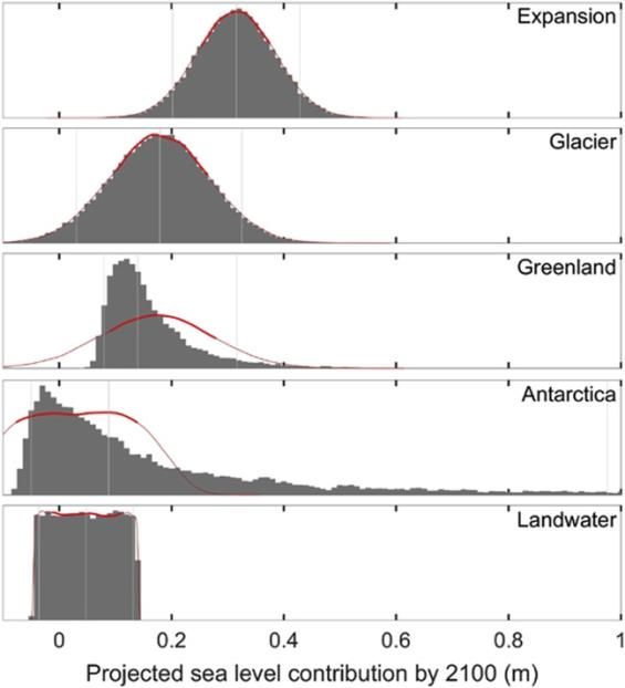
Below we discuss each of the four components of GMSL in greater detail.

Thermal Expansion
Between 1971 and 2010, the ocean absorbed 93% of the energy increase associated with human-induced climate change
(Church et al., 2013a). During that time, the upper ocean (i.e., top ~250 ft) warmed an average rate of 0.2°F per decade
(Rhein et al., 2013). As ocean temperatures increase, the density of seawater decreases and its volume increases,
causing sea level to rise in proportion with the heat content of the ocean (Church et al., 2013a). The IPCC’s AR5 projects
that thermal expansion will contribute a median 0.66 ft (likely range: 0.49 to 0.82 ft) of sea level rise by 2100 for RCP 4.5
relative to 1986-2005, and a median 1.05 ft (likely range: 0.82 to 1.28 ft) for RCP 8.5. Considering all greenhouse gas
scenarios evaluated in the AR5 (SRES A1B, RCP 2.6, RCP 4.5, RCP 6.0, RCP 8.5), thermal expansion accounts for between
30 and 55% of the projected change in end-of-century global sea level (Figure 1). More information on greenhouse gas
scenarios and likelihood terminology is provided in the call-out box on “The IPCC, GCMs, GHG Scenarios, Likelihood
Terminology.”

Appendix B: Global and Regional Sea Level Rise: A Review of the Science Page 3 of 46

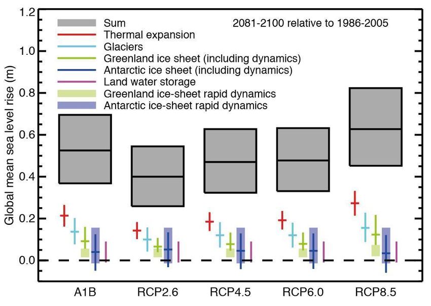
Using a probabilistic approach, Kopp et al. (2014) project changes in global sea level from thermal expansion by
developing a t-distribution where the mean and covariance matches the ensemble of GCM projections from CMIP5.
Before fitting the t-distribution, the authors apply a correction for model drift: models exhibit a large range of sea level
rise rates, even in the late nineteenth century when anthropogenic effects are expected to be minimal. To correct for

 FIGURE 1: Under all scenarios evaluated in the IPCC AR5 thermal expansion is the largest
 contributor to GMSL by the 2090s (2081-2100). This plot shows individual component and
 summed GMSL projections from process-based models for the 2090s relative to 1986-2005 for
 A1B and four RCP scenarios (2.6, 4.5, 6.0, 8.5). Gray boxes show the sum of individual
 components of sea level rise, with the horizontal bar representing the median projection and the
 height of the rectangle representing the likely range (Church et al., 2013a). Reproduced with
 permission.

this, Kopp et al. (2014) applied a linear correction so that the global mean rate of sea level rise matched the
observationally-based estimate of 0.01 ± 0.04 inches/year (95% confidence limits) for the years 1861-1900. This
correction was then applied to the full time series of GMSL for each model, extending through 2200.

Appendix B: Global and Regional Sea Level Rise: A Review of the Science Page 4 of 46

Kopp et al. (2014) project that thermal expansion will contribute a median 0.85 ft (likely range: 0.59 to 1.12 ft) of sea
level rise by 2100 under RCP 4.5 relative to 2000, and a median 1.21 ft (likely range: 0.92 to 1.51 ft) of sea level rise
under RCP 8.5. In addition to developing projections for the likely range, the authors also present their 5-95th percentile
projections for the contribution of thermal expansion to GMSL in 2100: 0.43 to 1.31 ft under RCP 4.5; and 0.72 to 1.71 ft
under RCP 8.5. Additional likelihood ranges for Kopp et al.’s (2014) thermal expansion projections are shown in Table 1.

Kopp et al.’s (2014) likely range is wider than the likely range of AR5 for both RCP 4.5 and 8.5. One explanation proposed
by Kopp et al. (2014) to account for this discrepancy is the correction they employed to account for model drift. In
addition to the drift correction, Kopp et al. (2014) posit that the use of the year 2000 as a baseline versus the AR5’s 1986-
2005 reference could account for some difference between the likely range of two projections.

The National Research Council (NRC) report (2012)2 used the output of GCMs to project the “steric” (which primarily
refers to thermal expansion) contribution to SLR. The NRC (2012) projections show an average sea level rise of 0.79 ft (1-
 range: 0.59 to 0.98 ft) by 2100, relative to 2000, for a moderate (A1B) greenhouse gas scenario (see the call-out box on
“The IPCC, GCMs, GHG Scenarios, Likelihood Terminology” for more information on how previous scenarios relate to the
latest greenhouse gas scenarios).

Thermal expansion numbers from Pfeffer et al. (2008) are included in Table 1 due to their relevance to the discussion on
the upper limits of 21st century sea level rise. Pfeffer’s estimated thermal expansion contribution to sea level rise is 0.98
ft and does not include uncertainty ranges. This estimate is based on the IPCC’s fourth assessment report (AR4; Meehl et
al., 2007).

2 Organized by a committee of scientists, the NRC study evaluated the effect of sea level rise at the global level and the regional level, focusing
 on the coasts of California, Oregon, and Washington for 2030, 2050, and 2100.

Appendix B: Global and Regional Sea Level Rise: A Review of the Science Page 5 of 46

TABLE 1: Comparing thermal expansion projections from IPCC’s AR5 (Church et al., 2013a), Kopp et al. (2014),
 NRC (2012), and Pfeffer et al. (2008). Projections are organized by greenhouse gas scenario (see Box 1,
 below). All projections are for the year 2100. The Pfeffer et al. reference is included because of its relevance
 to the discussion on the upper limits of 21st century sea level rise. Kopp et al. use the less-than symbol (“

Box 1. The IPCC, GCMs, GHG Scenarios, Likelihood Terminology

The IPCC
The Intergovernmental Panel on Climate Change (IPCC) is the leading intergovernmental scientific body that assesses the
current state of knowledge about climate change.

Since its establishment in 1988, the IPCC has released five Assessment Reports (ARs) that provide up-to-date syntheses
of the latest climate science research. The Assessment Reports address the drivers of climate change, provide climate
change projections, and discuss the potential impacts of climate change and options for response. These reports are
typically released every five to seven years, with the most recent Assessment Report (AR5) being released in 2013
(Church et al., 2013a), and the Sixth Assessment Report (AR6) scheduled for publication in 2021.

Global Climate Models
Climate change projections in the IPCC’s fourth and fifth Assessment Reports (AR4 and AR5, respectively) were
developed using Global Climate Models (GCMs) that are driven by future greenhouse gas scenarios. GCMs are a critical
tool used to simulate current climate and to project changes in climate under different greenhouse gas (GHG) scenarios
(Jiang et al., 2012). The World Climate Research Program organizes the Coupled Model Intercomparison Project (CMIP),
which establishes a standardized experimental framework for evaluating and interpreting GCM outputs. The most recent
phases of CMIP are phase 3 (CMIP3) which was used in the fourth assessment report (AR4), and phase 5 (CMIP5) which
was used in AR5 (Church et al., 2013a). CMIP5 included GCMs with higher spatial resolution than CMIP3, and also
generated a larger number of simulations (Sun et al., 2015).

Greenhouse Gas Scenarios
Atmospheric concentrations of greenhouse gases are affected by changes in global population, technological innovation,
economic development, and a host of other factors. Climate projections from both CMIP3 and CMIP5 are produced using
a range of plausible scenarios of future greenhouse gas concentrations. GHG scenarios for AR5 incorporate four different
scenarios, ranging from an extremely low scenario, involving aggressive emissions reductions, to a high “business as
usual” scenario with continued acceleration in greenhouse gas emissions through the 21st century (Table 2). Although
the CMIP5 scenarios were developed using a different methodology and span a wider range of possible 21 st century
emissions, many are similar to GHG scenarios used in CMIP3.

Appendix B: Global and Regional Sea Level Rise: A Review of the Science Page 7 of 46

TABLE 2: Previous greenhouse gas scenarios have close analogues in the new scenarios. Reproduced from
 Mauger et al. 2015. Current scenarios are from IPCC’s AR5 and VanVurren et al. 2011.

 Current Scenario characteristics Comparison to previous Terms used in this
 scenarios scenarios report

 RCP 2.6 An extremely low scenario that reflects No analogue in previous “Very Low”
 aggressive greenhouse gas reduction and scenarios
 sequestration efforts.

 RCP 4.5 A low scenario in which greenhouse gas Very close to B1 by 2100, “Low”
 emissions stabilize by mid-century and but higher emissions at
 fall sharply thereafter. mid-century

 RCP 6.0 A medium scenario in which greenhouse Similar to A1B by 2100, “Moderate”
 gas emissions increase gradually until but closer to B1 at mid-
 stabilizing in the final decades of the 21st century
 century.

 RCP 8.5 A high scenario that assumes continued Nearly identical to A1FI[1] "High”
 increases in greenhouse gas emissions
 until the end of the 21st century.

IPCC’s Likelihood Terminology
There will always be a range among climate projections. Uncertainties stem from a combination of three factors: natural
climate variability, model limitations, and our inability to predict the future of human emissions. In order to
communicate the uncertainties associated with an observed climate trend or projected change in a climate metric, the
IPCC employs calibrated “likelihood” terminology in which certain words or phrases are used to refer to specific
probabilities (Table 3). This likelihood language aims to assist in both the interpretation and communication of
uncertainties in climate science.

Appendix B: Global and Regional Sea Level Rise: A Review of the Science Page 8 of 46

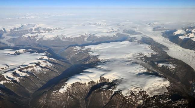
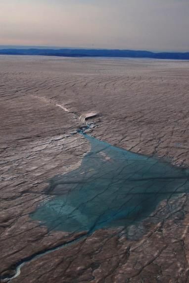
TABLE 3: Calibrated likelihood terminology and
 associated probability.

 Likelihood Scale

 Term Likelihood of the Outcome

 Virtually certain 99-100% probability

 Very likely 90-100% probability

 Likely 66-100% probability

 About as likely as not 33-66% probability

 Unlikely 0-33% probability

 Very unlikely 0-10% probability

 Exceptionally unlikely 0-1% probability

Land-Based Glaciers and Ice Sheets

Glaciers
Both glaciers and ice sheets contribute to sea level rise via changes in their mass balance – the net difference between
accumulation and loss of ice (Figure 2). A positive mass balance indicates that a glacier is expanding and a negative mass
balance indicates glacial retreat.

Surface mass balance is affected by both changes in
precipitation (affecting accumulation) and
temperature (affecting loss via both melt and
vaporization). At the glacier surface, changes are
governed by the balance at the surface (or “surface
mass balance”, hereafter SMB). SMB is measured by
calculating the difference between accumulation and FIGURE 2: Peripheral glaciers and ice caps from the eastern
 section of the Greenland Ice Sheet (visible in the top-right
ablation (the combination of melt and vaporization).
 corner of this photograph). Photo credit: NASA Goddard
In addition to changes in SMB, dynamic discharge – Space Flight Center, used under CC BY 2.0).

Appendix B: Global and Regional Sea Level Rise: A Review of the Science Page 9 of 46

the process by which ice breaks off of a glacier terminus; hereafter referred to as “Dynamical Change” – could be an
important contributor to future sea level rise on shorter time scales (decades to centuries; Church et al., 2013a).
However, the long-term potential contribution of glacial dynamic discharge to SLR is limited by the small overall volume
of global glacier ice, relative to the Greenland and Antarctic ice sheets. In addition, the observations required to project
glacial dynamic contributions to GMSL are unavailable at this time (Church et al., 2013a). As a result, contributions from
glacier dynamics were not included in AR5 projections of GMSL by 2100.

The IPCC’s AR5 projected the SMB changes of glaciers (excluding Antarctica3) using a scheme that was based on the
results of four global glacier models (Slagen & van de Wal, 2011; Marzeion et al., 2012; Giesen & Oerlemans, 2013; Radic
et al., 2014). These models present the glacial contribution to sea level as a function of time for a subset of CMIP3 and
CMIP5 GCMs. Several studies have projected SMB using an empirical approach, in which a statistical relationship is
developed relating temperature, precipitation, and atmospheric transmissivity--a measure of the “clearness” of the
atmosphere that is expressed as a ratio between the solar radiation outside the Earth’s atmosphere and solar radiation
on the land surface--to SMB. This relationship is then used to project changes in SMB in the future (Giesen and
Oerlemans, 2013; Marzieon, 2012; Radic et al., 2014; Slagen and van de Wal, 2011).

The IPCC’s AR5 projects a median sea level contribution of 0.43 ft (likely range: 0.23 to 0.66 ft) by 2100 – for RCP 4.5,
relative to 1986-2005 – for all global glaciers outside of Antarctica. For RCP 8.5 the projected change is 0.59ft (likely
range: 0.33 to 0.85 ft; Table 4). These changes correspond to a 15 to 55% loss of current glacial volume outside of
Antarctica by the year 2100 (Church et al., 2013a).

To project the non-Antarctic glacier and ice cap contribution to GMSL, Kopp et al. (2014) generate a multivariate t-
distribution with the mean and covariance estimated from the process based model results from Marzeion et al. (2012),
who use a statistical relationship between temperature and precipitation and changes in global glacier volume.

Kopp et al. (2014) projected that non-Antarctic glaciers will contribute a median 0.43 ft (likely range: 0.33 to 0.56 ft) of
sea level rise by 2100 under RCP 4.5, relative to 2000, and 0.59 ft (likely range: 0.46 to 0.69 ft) under RCP 8.5 relative to
2000. In addition to developing projections for the likely range, Kopp et al. also present their 5-95th percentile projections
for non-Antarctic glaciers contribution to GMSL in 2100; 0.23 to 0.62 ft under RCP 4.5 relative to 2000; and 0.36 to 0.79 ft
under RCP 8.5 relative to 2000. Additional likelihood ranges for Kopp et al.’s (2014) non-Antarctic glacier projections are
shown in Table 4.

The Kopp et al. (2014) projections have a narrower range than those in IPCC’s AR5. This difference likely originates from
the different glacier models which were selected for each of these studies. Kopp et al. (2014) chose to use the Marzeion

3 Antarctica’s peripheral glaciers were excluded from the global glacier models because the coverage of Climate Research Unit (CRU) datasets
 do not extend to Antarctica (Marzeion et al. 2012), and Antarctic peripheral glacier contribution is extremely uncertain (Slagan et al. 2017).
 The IPCC’s AR5 included projected changes in the mass and surface area of Antarctic peripheral glaciers within the Antarctic SMB estimate.

Appendix B: Global and Regional Sea Level Rise: A Review of the Science Page 10 of 46

et al. (2012) projections because of the ability to assess changes separately for 19 individual regions across the globe,
whereas the IPCC approach considered only the global average.

The National Research Council (NRC) report (2012) extrapolated observational mass balance data (Dyurgerov & Meier,
2005; Cogley, 2009; Dyurgerov, 2010) for glaciers and ice caps using a generalized linear model approach. Data were
assumed to be normally distributed and a weighted least squares approach was used to estimate model parameters
(NRC, 2012). The authors project that glaciers and ice caps will contribute a 0.46 ft (1- : 0.46 to 0.49 ft) of sea level rise
by 2100 under a moderate (A1B) greenhouse gas scenario, relative to 2000 (Table 4; for more on greenhouse gas
scenarios, see the call-out box on “The IPCC, GCMs, GHG Scenarios, Likelihood Terminology.”)

 TABLE 4: Comparing land-based glacial and ice cap projections from IPCC (Church et al., 2013a), Kopp et al.
 (2014), and NRC (2012). Projections are organized by greenhouse gas scenario (see Box 1, above). All
 projections are for the year 2100. Kopp et al. (2014) use the less-than symbol (

Kopp et al., 2014 5-95% range 2000 0.36-0.79 ft

 Kopp et al., 2014 0.5-99.5% range 2000 0.23-0.95 ft

 Kopp et al., 2014 Upper 99.9% 2000

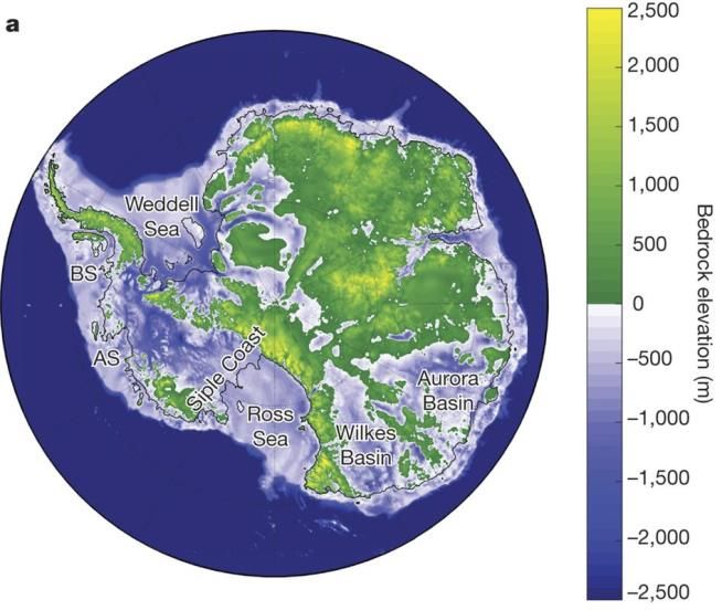
important conduit for meltwater because they are able to form across the entire glacial surface, whereas moulins only
form in the melt zone (Fountain & Walder, 1998). This flow of water through the glacier can reduce the viscosity of the
ice and allow it to move more quickly across the landscape (Phillips et al., 2010).

At the ice sheet margins, increasing subsurface ocean temperatures are a driver of peripheral ice sheet melt on
Antarctica and at a few locations in Greenland. Subsurface ocean waters come into contact with the bottom of floating
ice shelves and the edge of the ice sheet, thus exposing them to possible melt. When these bring warmer waters, they
result in a thinning of the ice shelves and a reduced buttressing effect on the ice sheet’s interior (Pollard et al., 2015;
Deconto & Pollard, 2016).4 The warmer waters also come into contact with the grounded edge of the ice sheet,
potentially causing it to retreat as it melts.

Exposure to warm subsurface ocean waters can only affect marine ice sheets that are grounded on bedrock below sea
 level. Large portions of the West Antarctic Ice Sheet
 (WAIS) lie on bedrock below sea level (Figure 4)
 (DeConto & Pollard 2016). The IPCC’s AR5 indicated
 that majority of the Greenland Ice Sheet (GIS) rests on
 bedrock above sea level (Church et al., 2013a),
 however, recent studies of GIS bedrock topography
 (Morlighem et al., 2014) suggest that there are
 significant ice-covered valleys that extend below sea
 level, indicating that some parts of Greenland are also
 vulnerable to warming ocean waters. This effect is
 particularly significant in basins where the “grounding
 line” – the boundary between where an ice sheet sits
FIGURE 4: Much of the Antarctic Ice Sheet lies on bedrock on bedrock and where floating ice shelves begin –
below sea level. Blue shading indicates bedrock elevations occurs on reverse-slope beds below sea level. The
below sea level and green shading indicated bedrock
 term “reverse-slope beds” refers to situations where
elevations above sea level. The regions below sea level are
susceptible to a positive feedback known as marine ice the ground underneath an ice sheet slopes downward
sheet and ice cliff instabilities. Figure Source: DeConto & towards the interior of the continent, away from the
Pollard 2016. Reproduced with permission. coast. Basins sitting on reverse-sloped beds are
 potentially unstable since a retreat of the grounding
line causes more ice to be exposed to ocean waters (i.e., the ice sheet edge, where it meets the ocean, becomes taller).
This in turn results in greater melt, additional retreat of the grounding line, greater exposure to ocean melt, and so on.
This concept is referred to as “Marine Ice Sheet Instability” (MISI; Figure 5b,c).

4 Circumpolar Deep Water--a warm, saline mass of water beneath the Antarctic surface waters that occurs in the lower reaches of the
 Antarctic Circumpolar Current (Orsi et al., 1995) – has been identified as the driver of melt beneath the floating ice shelves in the Amundsen
 Sea and Bellingshausen Sea portions of the West Antarctic Ice Sheet (Steig et al., 2012; Cook et al., 2016).

Appendix B: Global and Regional Sea Level Rise: A Review of the Science Page 13 of 46

Two studies from 2014 suggest that the MISI positive feedback may already be underway on the WAIS. In a modeling
study, Joughin et al. (2014) found evidence that unstable retreat from MISI is already occurring on the Thwaites Glacier
in West Antarctica (Joughin et al., 2014). Although the Thwaites Glacier’s contribution to sea level rise is expected to be
moderate during the 21st century (0.04 inches/year). Moreover, the collapse of the
Thwaites system will not occur in isolation and will likely have significant destabilization implications for adjacent basins
in West Antarctica (Joughin et al., 2014). A separate study (Park et al., 2013) used satellite observations to show that

Appendix B: Global and Regional Sea Level Rise: A Review of the Science Page 14 of 46

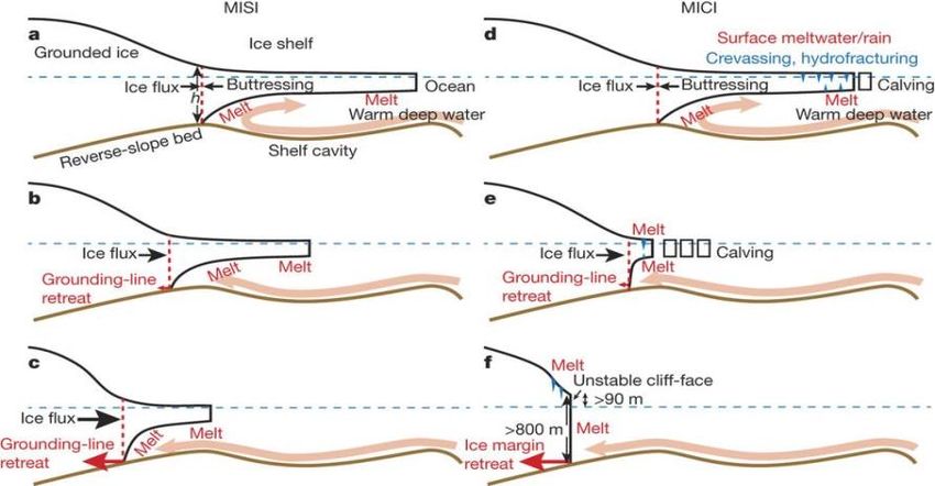
Figure 5. Schematic representation of marine ice sheet instability (MISI) and marine ice cliff instability
 (MICI). The three sequential figures on the left panel (a-c) show progressive ice retreat into a reverse-
 sloped bed driven by oceanic and atmospheric warming. The light pink arrow represents the
 movement of warm, salty water originating from the deep ocean into the shelf cavity. Figure a, shows
 a steady marine-terminating ice-sheet margin, with a floating ice shelf serving to buttress, or restrict
 outlet glacier flow (ice flux). The ice flux of the outlet glacier is heavily dependent on the thickness of
 the grounding-line (i.e., ice flux is faster with a thicker grounding line). b, The infiltration of warm
 ocean water into the shelf cavity increases ice melt on the bottom of the ice shelf, causing thinning.
 As ice shelves thin, their buttressing effect decreases, which causes an increase in ice flux, and
 subsequent grounding line retreat onto a reverse-sloped bed. c, As grounding line thickness increases
 and grounding line retreat into the reverse-sloped bed continues, ice flow across the grounding line
 will continue to increase unabated until the reverse-sloped bed levels out. d, In addition to MISI (a–c),
 the ice sheet model used by DeConto & Pollard (2016) modeled calving events driven by surface
 meltwater and the hydrofracturing of floating ice (e), these crevassing and hydrofracturing events
 shorten the ice shelf length and accelerate grounding-line retreat into deep, reverse-sloped beds. f. In
 some instances oceanic melt and calving may completely remove ice shelves, exposing drastic cliff
 faces at the ice margin which become structurally unstable once they exceed 2,625 ft, leading to
 runaway retreat into reverse-sloped beds. Figure source: Pollard & DeConto, 2016. Reproduced with
 permission.

between 1992 and 2011 the Pine Island Glacier (PIG), adjacent to Thwaites in West Antarctica, retreated by tens of
kilometers. Currently, the grounding line of PIG is sitting on bedrock with a reverse-sloped bed, increasing the likelihood
that irreversible retreat associated with MISI is currently underway for PIG. Favier et al. (2014) find evidence supporting
this hypothesis by using three different ice-flow models to investigate (1) whether the bedrock topography of the WAIS
basin is driving the dynamic response of PIG and (2) if grounding line stabilization is possible on the reverse-sloped bed.

Appendix B: Global and Regional Sea Level Rise: A Review of the Science Page 15 of 46

All three ice-flow models suggest that MISI is occurring in PIG, and two out of three ice-flow models suggest that this
retreat is unlikely to stabilize.

Satellite radar interferometry has been used to document rapid grounding line retreat of the Pine Island, Thwaites,
Smith, and Kohler glaciers in the Amundsen Sea sector of West Antarctica between 1992-2011 (Rignot et al. 2014). The
retreat of these glacial grounding lines occurred on reverse-sloped beds below sea level and is unlikely to stabilize
without a significant increase in ice shelf buttressing, which is considered unlikely. This retreat is expected to continue
over the coming decades and centuries, contributing significantly to sea level rise (Rignot et al., 2014).

Observational data from Jakobshavn Isbræ – Greenland’s fasted flowing glacier – shows that the glacier’s speed has
accelerated rapidly over the past 15 years and that the glacial terminus has retreated into a basin that sits more than
4,265 ft below sea level (Joughin et al., 2014). As with the Thwaites and Pine Island glaciers, the reverse-slope bed
suggests that continued retreat is likely (Joughin et al., 2014).

In addition to MISI, warming subsurface ocean waters can lead to ice shelf undercutting, increased calving events, cliff
failure, and ice margin retreat. This mechanism, which results in structural failure at the grounding line, was initially
introduced by Bassis and Walker (2012) and has more recently been referred to as “Marine Ice Cliff Instability” (MICI;
Figure 5 d-f; Vaughan et al., 2013; Pollard, 2015; DeConto and Pollard, 2016). As the buttressing effect of ice shelves is
lost, grounding line retreat on a reverse-sloped bed can expose cliff faces taller than 295 ft, potentially leading to a
structural failure as ice-cliffs become too tall (Figure 2; right panel; Bassis and Walker, 2011; Pollard et al., 2015; DeConto
and Pollard, 2016).

A recent study (Wise et al., 2017) presented the first observational evidence of the MICI mechanism occurring in Pine
Island Bay in a similar manner to what was discussed in the recent DeConto and Pollard (2016) paper. The study
evaluated iceberg keel-plough marks on the seafloor offshore of the WAIS ice sheet, which provides information on
historic iceberg shape and drift direction. Since they involve scouring the ocean floor, these keel-plough marks can only
occur when ice breaks off the grounded ice sheet – the ice shelves, since they are floating, do not touch the ocean floor.
This suggests that MICI is the primary mechanism responsible for the historic ice-sheet retreat in the Pine Island Bay that
occurred between 12,300-11,200 years ago.

Greenland Ice Sheet (GIS) | Surface Mass Balance
The IPCC’s AR5 projects that changes in the SMB of the Greenland Ice Sheet will contribute a median 0.16 ft (likely range:
0.07 to 0.36 ft) of sea level by 2100 for RCP 4.5, relative to 1986-2005, and a median 0.33 ft (likely range: 0.13 to 0.72 ft)
of sea level by 2100 for RCP 8.5. Projections are based on a published relationship (Fettweis et al. 2013) that relates
surface mass balance to surface temperature. This relationship is derived from simulations of the MAR (Modèle
Atmosphérique Régional; Gallée & Schayes, 1994) regional climate model, forced by three GCMs for RCP 4.5 and RCP 8.5
(van Vuuren et al., 2011; Fettweis et al., 2013). The SMB height feedback is expected to contribute an additional 0 to 15%

Appendix B: Global and Regional Sea Level Rise: A Review of the Science Page 16 of 46

of projected SMB mass loss by 2100 (between 0 to 0.55 inches of sea level rise by 2100 based on the SMB projection for
RCP 8.5).

Greenland Ice Sheet (GIS) | Change in Ice Dynamics
In the IPCC’s AR5, the 21st century sea level contribution from Greenland’s change in ice dynamics were estimated by
fitting a quadratic function of time between the start of the projections (taken to be half the observed rate of loss
between 2005-2010) and the upper and lower limits of estimated SLR contribution by 2100. The upper limit of the
estimated contribution is based primarily on Nick et al. (2013), which focused on a subset of Greenlands’ glaciers. For the
IPCC projections, the Nick et al. (2013) results were scaled up by a factor of ~5 to correspond to changes for the entire
ice sheet (the Nick et al. (2013) study only modeled about one fifth of the Greenland ice sheet; Church et al., 2013a). The
lower limit of these estimates is derived from Nick et al. (2013) and Goelzer et al. (2013). The ice dynamic contribution
time series were generated between these upper and lower extremes, and a constant representing the estimated
contribution between 1996-2005 (0.06 inches) was added to account for the additional change prior to the start of the
projections.

The IPCC’s AR5 projected that dynamic changes in the GIS will contribute a median 0.13 ft (likely range: 0.03 to 0.2 ft) of
sea level by 2100 under RCP 4.5 relative to 1986-2005, and a median 0.16 ft (likely range: 0.07 to 0.30 ft) of sea level by
2100 under RCP 8.5 relative to 1986-2005.

Greenland Ice Sheet Contribution to Global Sea Level |
(Ice Dynamics + SMB)
After combining contributions from SMB and rapid dynamics, the IPCC’s AR5 projected that mass loss from the GIS will
contribute a median 0.3 ft (likely range: 0.20 to 0.52 ft) of sea level rise by 2100 under RCP 4.5 relative to 1986-2005, and
a median 0.49 ft (likely range: 0.30-0.92 ft) under RCP 8.5 relative to 1986-2005 (Table 5). SMB projections were derived
using RCM or downscaled AOGCM simulations.

The IPCC’s analysis does not quantify the interaction between SMB and dynamic ice loss (i.e., thinning of the ice sheet
due to surface melt can reduce the rate of calving). A recent study by Fürst et al. (2015) used an ice flow model that
captures the combined impacts of SMB and dynamic changes, as well as the interactions between the two. Fürst et al.
(2015) project a contribution to sea level between and 0.13-0.23 ft (1-standard deviation range) to sea level by 2100
under RCP 4.5 relative to 2000, and 0.23-0.43 ft (1 standard deviation range) to global sea level by 2100 relative to 2000
under RCP 8.5. These projections are lower than those from the IPCC’s AR5, likely because the interaction between SMB
and ice dynamics is included.

Kopp et al. (2014) used the IPCC AR5 estimates of the median and likely ranges (central 66% of the probability
distribution) of total ice sheet losses, but the expert elicitation of Bamber and Aspinall (2013) to define the shape of the
tails (lower and upper 17 percent of the probability distribution). The resulting projections show GIS contributing a

Appendix B: Global and Regional Sea Level Rise: A Review of the Science Page 17 of 46

median 0.30 ft (likely range: 0.13-0.49 ft) to sea level rise under RCP 4.5, and a median 0.46 ft (likely range: 0.26-0.82 ft)
by 2100 under RCP 8.5, all relative to 1986-2005. Kopp et al. (2014) did not separate out surface mass balance and ice
dynamics for the GIS.

 TABLE 5: Comparing projections of Greenland Ice Sheet contribution to global sea level rise from IPCC AR5,
 Church et al. (2013a), Kopp et al. (2014), Fürst et al. (2015) and NRC (2012). Projections are organized by
 greenhouse gas scenario (see Box 1, above for more information on scenarios). All projections are for the year
 2100. Kopp et al. (2014) use the less-than symbol (

NRC, 2012§ Range of all scenarios 2100, relative to 2000 0.49-1.12 ft

‡ The NRC projections are assessed relative to the year 2000 for a moderate (A1B) greenhouse gas scenario.
§ The range of NRC projections for B1-A1FI.

Antarctic Ice Sheet (AIS) | Surface Mass Balance
IPCC’s AR5 projects that SMB changes to the AIS during the 21st century will be solely due to changes in accumulation.
Previous studies have projected only slight changes in Antarctic surface losses because the surface of the ice sheet is
rarely above freezing and when melt does occur it is often captured by refreezing (Ligtenberg et al., 2013). Accumulation,
however, is projected to increase as a result of greater snowfall, driven primarily by the increased water holding capacity
of a warmer atmosphere. As a result, SMB on the AIS is expected to have a negative contribution to sea level rise over
the 21st century (i.e., increased accumulation at the surface of the ice sheet removes mass from the ocean). Since the
effect is primarily linked to warming, not changes in circulation, the AR5 used surface temperature projections to
estimate a median -0.10 ft (likely range: -0.2 to -0.03 ft) contribution to sea level by 2100 under RCP 4.5 relative to 1986-
2005, and a median -0.16 ft (likely range: -0.3 to -0.07 ft) contribution to sea level by 2100 for RCP 8.5 relative to 1986-
2005 (Church et al., 2013a).

Antarctic Ice Sheet (AIS) | Changes in Ice Dynamics
For changes in ice dynamics, the IPCC’s AR5 assessed the likely range of sea level contributions from Antarctica by fitting
a quadratic function of time between the start of the projections (taken to be the observed rate of loss between 2005-
2010) and the upper and lower limits of estimated SLR contribution by 2100. These limits were based primarily on Little
et al. (2013), who employed a probabilistic framework to estimate the upper and lower bounds of changes in Antarctic
ice loss by 2100. The AR5 projections amount to a median contribution of 0.26 ft (likely range: -0.07 to 0.62 ft) of sea
level by 2100 relative to 1986-2005. The same projection is used for all greenhouse gas scenarios.

Antarctic Ice Sheet Contribution to Global Sea Level
(Ice Dynamics + SMB)
The AIS is the largest potential contributor to GMSL (Church et al. 2013a) and is also the most uncertain (Levermann et
al., 2014). The AR5 projection for the combined changes in SMB and changes in ice sheet dynamics is a median 0.13 ft
(likely range: -0.26 to 0.46 ft) increase in global sea level by 2100 relative to 1986-2005 for RCP 8.5, and a median 0.16 ft
(likely range: -0.16 to 0.49 ft) for RCP 4.5 (Church et al., 2013a; Table 6). The report goes on to say that global sea level
would only substantially exceed the likely range of GMSL by 2100 (likely range: 1.70 to 3.22 ft) if marine-based sectors of
the AIS collapse. As noted above, the authors state that although there is a potential for such a collapse, scientific
understanding is currently insufficient to estimate the probability that it will occur, or the speed at which it will proceed.

Since the release of AR5 significant strides have been made in understanding and modeling the dynamic processes and
resulting sea level contributions of the AIS. For example, Levermann et al. (2014) employed a probabilistic approach for

Appendix B: Global and Regional Sea Level Rise: A Review of the Science Page 19 of 46

estimating Antarctic ice discharge originating from discharge driven by basal ice-shelf melting (melt occurring at the
interface of the ice sheet and the underlying bedrock). Specifically, the authors developed projections from three ice
sheet models from the Sea-Level Response to Ice Sheet Evolution (SeaRISE) project using linear response theory. The
authors projected that dynamic changes to the AIS would contribute a median 0.30 ft (likely range: 0.13 to 0.69 ft; 95%
range: 0.03 to 1.21 ft) to sea level by 2100 under RCP 8.5 relative to 2000 (Table 6). This likely range is similar but slightly
wider than the likely range presented in the IPCC’s AR5.

Ritz et al. (2015) tested a process-based ice-sheet model against a wide range of model assumptions, comparing each
with observed mass loss in the Amundsen sea embayment from 1992-2011. Using the model configurations that best
matched the observations, these were used to estimate the probability distribution of future mass loss for the entire
Antarctic ice sheet. Their results project a contribution of up to 0.98 ft (95% quantile) of SLR by 2100 for the moderate
A1B scenario. The authors also conclude that Antarctic contributions to GMSL of ~3.3 feet or more are physically
impossible. However, recent studies how suggested that contributions that exceed three feet are possible and should be
considered likely (DeConto and Pollard, 2016).

Kopp et al. (2014) used the IPCC’s AR5 estimates of the median and likely ranges (central 66% of the probability
distribution) of total ice sheet losses, but the expert elicitation of Bamber and Aspinall (2013) to define the shape of the
tails (lower and upper 17 percent of the probability distribution). The resulting projections show the Antarctic Ice Sheet
contributing a median 0.16 ft (likely range: -0.16-0.52 ft) to sea level rise under RCP 4.5, and a median 0.13 ft (likely
range: -0.26 to 0.49 ft) by 2100 under RCP 8.5, all relative to 1986-2005 (Table 6). Kopp et al. (2014) did not separate out
surface mass balance and ice dynamics for the AIS.

Existing ice sheet models are not able to reproduce the large changes in sea level that are implied by the geologic
record. Specifically, geologic records indicate that sea levels have varied significantly over the past ~25 million years,
reaching more than ~66 ft above present sea surface heights (with comparable CO2 concentrations to today, Naish et al.,
2009). If these geological data are correct, this indicates that the East Antarctic Ice Sheet (EAIS) has contributed
significantly to past sea levels (~20-30% of the current volume of EAIS). Ice-sheet models have thus far been unable to
show significant retreat of the EAIS, typically estimating changes in global sea level that are about a factor of ten smaller
than the geologic evidence suggests. Pollard et al. (2015) updated an existing three-dimensional model (DeConto et al.,
2012) to incorporate the two mechanisms necessary to cause large ice cliff failure (i.e., Marine Ice Cliff Instability, or
MICI; see discussion above), (1) surface water driven hydrofracturing, and (2) structural failure at the grounding line. To
do this, the authors added simplified representations of these mechanisms based on observations and previous work.
The ice sheet model was run with a simple Pliocene-like ocean warming scenario of +3.6°F (+2°C), which resulted in a
quick collapse of the West AIS, on the order of decades. Over longer periods of time (several hundred to a few thousand
years) significant retreat of the EAIS was also simulated. The +3.6°F (+2°C) ocean warming may be unrealistically high
since it is at the high end of the projections of global average ocean temperatures, and there is evidence that the ocean
waters surrounding Antarctica will warm less rapidly than other parts of the globe (Collins et al., 2013). Although the

Appendix B: Global and Regional Sea Level Rise: A Review of the Science Page 20 of 46

modeling approach is simplified, it is the first time a model has been able to produce changes in sea level that are
consistent with the geologic record. The authors also highlight that the model results suggest that the EAIS may be more
sensitive to warming than previous ice sheet models suggested.

DeConto and Pollard (2016) built off the Pollard et al. (2015) AIS model by improving the representation of calving, the
effects of surface melt water, and the link to oceanic and atmospheric changes. In order to account for the uncertainties
in the new modeling approach, the authors tested a variety of model configurations, comparing each to the
observationally-based estimates of sea level rise during the Pliocene (about 3 million years ago) and the Last Interglacial
(about 100,000 years ago). The model configurations that resulted in a good match were used to develop a set of future
projections for each greenhouse gas scenario. Since there is some uncertainty in the Pliocene estimates of sea level, the
authors provide two sets of future projections. The low-end projections, which assume that Pliocene sea level was 16-49
ft higher than today, project that AIS will result in a sea level rise of 0.85 ft (likely range: -0.07 to 1.77 ft) for RCP 4.5 and
2.10 ft (likely range: 0.49 to 3.71 ft) for RCP 8.5 by the year 2100 relative to 2000. If instead the high-end Pliocene
estimates are used (Pliocene sea level is 33-66 ft higher than today), the authors project a rise of 1.61 ft (likely range:
0.95 to 2.26 ft) for RCP 4.5 and 3.44 ft (likely range: 2.46 to 4.43 ft) for RCP 8.5, again for the year 2100 relative to 2000.
Although this study highlights important mechanisms that may lead to accelerated Antarctic melt, the authors note that
their results are preliminary and “should not be viewed as actual predictions.”

 TABLE 6: Comparing projections of Antarctic Ice Sheet contribution to global sea level rise from IPCC AR5,
 Church et al. (2013a), Kopp et al. (2014), Levermann et al. (2014), Ritz et al. (2015) and NRC (2012).
 Projections are organized by greenhouse gas scenario (see Box 1, above for more information on scenarios).
 All projections are for the year 2100. Kopp et al. (2014) use the less-than symbol (

RCP 8.5

 IPCC’s AR5 66% range 2100, relative 1986-2005 -0.26-0.46 ft

 Kopp et al., 2014 66% range 2100, relative to 2000 -0.26-0.49 ft

 Levermann et al., 66% range 2100, relative to 2000 0.13-0.69 ft
 2014

 Levermann et al., 5-95% range 2100, relative to 2000 0.03-1.21 ft
 2014

 Kopp et al., 2014 5-95% range 2100, relative to 2000 -0.36-1.08 ft

 Kopp et al., 2014 0.5-99.5% range 2100, relative to 2000 -0.46-2.99 ft

 Kopp et al., 2014 99.9% 2100, relative to 2000

The AR5 also used two different methods to evaluate the contribution of water storage in reservoirs. The first method
estimated the rate of impoundment from water reservoirs between 1971-2010 (Lempérière and Lafitte, 2006) (mean:
0.008 inches yr-1; standard deviation: ±0.002 inches yr-1) and assumed this rate would continue through the 21st century
which resulted in an estimated mean: -0.06 ft (standard deviation range: -0.04 to -0.09 ft) by the 2090s (2081-2100),
relative to 1986-2005. The second method assumes the rate of impoundment of water in reservoirs to be zero after 2010
(i.e., no additional net impoundment—suggesting a balance between the construction of reservoir capacity and reduced
storage volume due to sedimentation). When combined, the two methods for projecting the influence of reservoir
storage on sea level range between 0 and -0.10 ft by the 2090s (2081-2100, relative to 1986-2005). After combining the
estimates from groundwater extraction and reservoir storage, the AR5 projects that land water storage will contribute a
median 0.16 ft (likely range: -0.03 to 0.36 ft) of sea level by 2100, relative to 1986-2100, irrespective of which
greenhouse gas scenario is considered (Table 7).

Since the release of AR5, new results from Wada et al. 2016 (the lead author of the groundwater estimates used in
IPCC’s AR5; Wada et al., 2012) suggest that the AR5 may have overestimated the contribution of groundwater extraction
to sea level rise by a factor of three (Wada et al., 2016). The authors state that this overestimation is the result of the
incorrect assumption that almost all extracted groundwater will return to the ocean. Using a coupled climate-
hydrological model (Wada et al. (2012) estimates were based on uncoupled land hydrological models), Wada et al.
(2016) find that only 80% of extracted groundwater returns to the oceans, a significantly lower fraction than what was
assumed in AR5 (nearly 100%). Recent research suggests that extracted groundwater used for irrigation enhances
precipitation downwind of irrigated areas (Wada et al., 2016).

Unlike the IPCC’s AR5, Kopp et al. (2014) estimate the contribution of land water storage to global sea level using a
relationship between population and water storage. Specifically, for changes in reservoir storage, Kopp et al. assume that
reservoir construction is sigmoidal function of population. When evaluating groundwater depletion, the authors fit the
estimates from Wada et al. (2012) and Kinihow et al. (2011) with linear functions of population. The projected rates of
groundwater depletion are driven by the United National Department of Economics and Social Affairs population
projections for the 21st century. Kopp et al. project that land water storage – which they calculate as the net effect of
reservoirs and groundwater extraction – will contribute between 0.10 to 0.23 ft (likely range) to global sea level by 2100,
using the same projections for all greenhouse gas scenarios. In addition to the likely range, the authors also give the 5th
to 95th percentile range of 0.07 to 0.26 ft by 2100, again using the same projection for all greenhouse gas scenarios
(Table 7). Kopp et al. (2014) likely range is narrower than the projected likely range of AR5. In fact, the upper end of the
AR5 likely range (0.36 ft) is in line with the 99.9th percentile estimate of Kopp et al. (2014).

 TABLE 7: Comparing projections of Antarctic Ice Sheet contribution to global sea level rise from IPCC AR5,
 Church et al. (2013a), and Kopp et al. (2014). All projections are for the year 2100. Kopp et al. (2014) use the
 less-than symbol (

Land Water Storage Contribution to Global Sea Level Rise

 Source Range Years Projection

 Irrespective of Greenhouse Gas Scenario

 IPCC’s AR5 66% range 2100, relative 1986-2005 -0.03-0.36 ft

 Kopp et al., 2014 66% range 2100, relative to 2000 0.10-0.23 ft

 Kopp et al., 2014 5-95% range 2100, relative to 2000 0.07-0.26 ft

 Kopp et al., 2014 0.5-99.5% range 2100, relative to 2000 0.0-0.36 ft

 Kopp et al., 2014 99.9% 2100, relative to 2000

Figure 6. Comparing global sea level projections (in feet) among recent studies. Shaded
 backgrounds indicate different percentile ranges: light blue encompasses the central 66
 percentile range; light yellow encompasses the central 90 percentile range; and light green
 encompasses two standard deviations from the mean from the NRC report and the central 99%
 range of Kopp et al. (2014). Dashed lines illustrate upper limit estimates from Kopp et al. (2014)
 Pfeffer et al. (2008), and the Pfeffer calculation that is driven by using Kopp’s 99.9th percentile
 values for thermal expansion and land water storage. Horizontal lines within bars represent
 median projections (Horton et al., 2014 did not provide median projections). Image credit:
 University of Washington Climate Impacts Group.

Kopp et al. (2014) project a likely GMSL range of 2.03 to 3.28 ft by 2100 under RCP 8.5 (relative to 2000), which is
comparable to the likely range from AR5 (likely range: 1.71 to 3.22 ft; relative to 1986-2005). Kopp et al.’s (2014)
projections for 2100 under RCP 4.5, 1.48 to 2.53 ft, are only slightly higher than those presented in the AR5 (likely range:
1.18 to 2.33 ft; RCP 4.5). In addition to developing projections for the likely range, the authors also provide results for
other probability levels, including the 5th and 95th percentiles for GMSL in 2100 (relative to 2000): 1.18 to 3.05 ft for RCP
4.5, and 1.71 to 3.97 ft for RCP 8.5. The 99.9th percentile estimate for GMSL in 2100 is 8.2 ft, relative to 2000, for RCP 8.5.
These high-end projections exceed the 6.56 ft upper limit of sea level estimated by Pfeffer et al. (2008), who used a
kinematic approach to evaluate constraints glaciological outflow rates (this study is discussed in greater detail in the

Appendix B: Global and Regional Sea Level Rise: A Review of the Science Page 25 of 46

“Upper Limits of Sea Level Rise” section, below). However, after incorporating Kopp et al.’s 99.9th percentile values for
thermal expansion and land-based water storage contribution to Pfeffer et al.’s (2008) calculations, the Pfeffer et al.
projection (8.10 ft) is in nearly exact agreement with Kopp et al.’s (2014) 99.9% projection of

and high (RCP 8.5) greenhouse gas scenario. For RCP 2.6, experts reported a median likely range between 1.31-1.97 ft,
and a median very likely range between 0.82-2.30 ft by 2100. For RCP 8.5 experts reported a likely range between 2.30-
3.94 ft, and a very likely range between 1.64-4.92 ft by 2100. The likely estimates from this broad expert elicitation are
higher than the likely range suggested by the AR5 for 2100 and RCP 8.5 (median value: 2.43 ft, likely range: 1.64 to 3.22
ft). Horton et al. also note that 13 of the 90 experts surveyed (~14% of the sample) “estimated a 17% probability of
exceeding 6.56 ft of sea level rise by AD 2100 under” RCP 8.5. The upper tail of the probability distribution is longer than
that of Kopp et al. (2014). As stated by Kopp et al. (2014): “The surveyed experts’ 83rd and 95th percentiles correspond
to our 95th and 99th percentiles, respectively.”

Semi-Empirical Model Approaches
SEMs derive statistical relationships between sea level and temperature from the observed historical record or longer
proxy records. This means that SEM projections are based on the straightforward assumption that the statistical
relationship between temperature or radiative forcing and sea level during the calibration period will continue to apply
as conditions change in the future. Given that many important processes – especially ice dynamic change on Greenland
and Antarctica – are not present in the historical record, the SEM approach of extrapolating those observations forward
could be problematic. In addition, many of the SLR projections generated by SEMs have historically been quite high
relative to process-based approaches. However, recent advancements and modifications of traditional SEM approaches
have reconciled the large gap between SEMs and process-based projections (Kopp et al., 2016; Mengel et al., 2016).

Rahmstorf (2007) was one of the first publications which used a semi-empirical modeling approach to generate SLR
projections for the 21st century. The author projects a likely range of 1.64 to 4.59 ft of sea level rise by 2100 (relative to
1990) based on a wide range of greenhouse gas scenarios (Nakicenovic et al., 2000). These projections are higher and
have a wider range than the likely GMSL range presented in AR5 (1.18-3.22 ft).

Two recent papers – Kopp et al. (2016) and Mengel et al. (2016) – have revisited the SEM approach. Mengel et al. (2016)
developed a novel, hybrid approach for generating sea level rise projections which employs both process-based and
semi-empirical modeling. The authors use past observations to calibrate three separate semi-empirical models, one each
for: (1) thermal expansion, (2) mountain glaciers, and (3) the Greenland and Antarctic ice sheets. Previous SEM
projections were generated by a single model which was calibrated by historical observations of total sea level rise. Using
this hybrid approach Mengel et al. (2016) project a median anthropogenic sea level contribution of 1.74 ft by 2100 for
RCP 4.5 (5th-95th percentile range: 1.21-2.53 ft), and 2.79 ft (5th-95th percentile range: 1.87-4.27 ft) for RCP 8.5. These
projections are similar to those developed for IPCC’s AR5.

Kopp et al. (2016) compiled a new database of relative sea level reconstructions for the Common Era (CE) from 24
locations globally, which were then broadened with records from 66 tide gauges. This database was analyzed with a
spatiotemporal empirical hierarchical model to estimate the common global sea level signal during the CE. The authors
then used this historical CE reconstruction to calibrate a SEM. The authors project a median global sea level rise of 1.67 ft

Appendix B: Global and Regional Sea Level Rise: A Review of the Science Page 27 of 46

(5th-95th percentile range: 1.08-2.79 ft) by 2100 for RCP 4.5, and 2.49 ft (5th-95th percentile range: 1.71-4.30 ft) for RCP
8.5. These newer SEM studies have resolved much of the discrepancy that has previously existed between the
processed-based and SEM projections.

 TABLE 8: Comparing projections of global sea level rise from IPCC AR5, Church et al. (2013a), Kopp et al.,
 (2014), Mengel et al. (2016), Horton et al. (2014), Miller et al. (2013), and NRC (2012). Projections are
 organized by greenhouse gas scenario (see Box 1, above for more information on scenarios). All projections are
 for the year 2100. Kopp et al. (2014) use the less-than symbol (

OTHER

 Jevrejeva et al., 2014 95% 2100 5.91 ft

 Miller et al., 2013* 95% 2100 5.90 ft

 Horton et al., 2014 (expert 5-95% range 2100 0.82-2.30 ft
 elic.) †

 Horton et al., 2014 (expert 66% 2100 1.31-1.97 ft
 elic.) †

 NRC, 2012‡ 2 std. Deviation from 2100, relative to 2000 2.36-3.05 ft
 mean

 NRC, 2012§ Range of all scenarios 2100, relative to 2000 1.64-4.27 ft

* Miller et al. (2013) projections are assessed for a high (A1FI) greenhouse gas scenario.
‡ The NRC projections are assessed relative to the year 2000 for a moderate (A1B) greenhouse gas scenario.
§ The range of NRC projections for B1-A1FI.
† The Horton et al. (2014) projections are assessed for an extremely low (RCP 2.6) greenhouse gas scenario.

Upper Limits of Sea Level Rise
In order to assess potential impacts and effectively plan for sea level rise, many decision-makers require reliable
estimates of the upper limit of possible sea level change. The likely range projections (central 66%) presented in the
IPCC’s AR5 do not include the lower probability, higher risk projections (highest 17% of projections) which may need to
be considered in certain management situations.

Pfeffer et al. (2008) was one of the first publications to develop kinematic constraints on the maximum about of sea level
rise, based on estimated rates of dynamic ice sheet loss. Following the IPCC’s AR4, which excluded dynamically forced
discharge from sea level rise projections (due to insufficient understanding of relevant processes at the time), Pfeffer et
al. (2008) calculated the discharge of marine-terminating outlet glaciers in Greenland and Antarctica required to reach
sea level targets of 6.56 ft and 16.4 ft by 2100. The authors concluded that increases in sea level greater than 6.56 ft are
physically impossible, however, a rise of ~6.56 ft is possible if glacier velocities rapidly increase. As a result of their
analysis, the authors present an ‘improved’ range (from what was presented in AR4) of GMSL by 2100 of between 2.62
and 6.56 ft. One limitation of the Pfeffer et al. (2008) projections is their use of a constant thermal expansion
contribution of 0.98 ft (based off Meehl et al., 2007) across all three scenarios considered. In addition, Pfeffer et al. do
not include a land water storage contribution to SLR in their analysis.

Kopp et al. 2014 use a probabilistic approach to estimate 21st century sea level rise. By using a probabilistic approach,
the authors are able to quantify the extremely low probability, high impact projections. Kopp et al. (2014) interpret their
99.9th percentile projections as an upper limit. For GMSL in 2100, these show a rise of