ESA Climate Change Initiative (CCI+) Essential Climate Variable (ECV) Antarctica_Ice_Sheet_cci+ (AIS_cci+)
←
→
Page content transcription
If your browser does not render page correctly, please read the page content below
Antarctica_Ice_Sheet_cci+ Reference: ST-UL-ESA-AISCCI+-ATBD-001
 Algorithm Theoretical Basis Document (ATBD) Version : 1.0 page
 for AIS CCI+ Phase 1 Date : 9 March 2020 1/48

 ESA Climate Change Initiative (CCI+)
 Essential Climate Variable (ECV)
 Antarctica_Ice_Sheet_cci+ (AIS_cci+)

 Algorithm Theoretical Basis Document (ATBD) for CCI+
 Phase 1

Prime & Science Lead: Andrew Shepherd
 University of Leeds, Leeds, United Kingdom
 a.shepherd@leeds.ac.uk

Technical Officer: Marcus Engdahl
 ESA ESRIN, Frascati, Italy
 Marcus.Engdahl@esa.int

Consortium: DTU Microwaves and Remote Sensing Group (DTU-N)
 DTU Geodynamics Group (DTU-S)
 ENVironmental Earth Observation GmbH (ENVEO)
 Deutsches Zentrum für Luft- und Raumfahrt (DLR) Remote Sensing Technology
 Institute (IMF)
 Science [&] Technology AS (ST)
 Technische Universität Dresden (TUDr)
 University College London (UCL/MSSL)
 University of Leeds, School of Earth and Environment (UL)
Antarctica_Ice_Sheet_cci+ Reference: ST-UL-ESA-AISCCI+-ATBD-001
 Algorithm Theoretical Basis Document (ATBD) Version : 1.0 page
 for AIS CCI+ Phase 1 Date : 9 March 2020 2/48

 Signatures page
Prepared Jan Wuite Date: 6 Mar 2020
by Lead Author, ENVEO

Issued by Daniele Fantin, Date: 6 Mar 2020
 Project Manager, S[&]T

Checked Andrew Shepherd Date: 9 Mar 2020
by
 Science Leader, UL

Approved Marcus Engdahl Date:
by ESA Technical Officer
Antarctica_Ice_Sheet_cci+ Reference: ST-UL-ESA-AISCCI+-ATBD-001
 Algorithm Theoretical Basis Document (ATBD) Version : 1.0 page
 for AIS CCI+ Phase 1 Date : 9 March 2020 3/48

 Table of Contents
Change Log ........................................................................................................... 5
Acronyms and Abbreviations ................................................................................ 6
1 Introduction ................................................................................................... 7
1.1 Purpose and Scope ......................................................................................... 7
1.2 Document Structure ....................................................................................... 7
1.3 Applicable and Reference Documents ................................................................ 7
2 Surface Elevation Change ............................................................................... 8
2.1 Introduction .................................................................................................. 8
2.2 Review of scientific background ........................................................................ 8
2.3 Algorithms................................................................................................... 10
 2.3.1 Plane fit ...............................................................................................................10
 2.3.2 Cross-calibration ...................................................................................................12
2.4 Input data and algorithm output .................................................................... 13
2.5 Accuracy and performance ............................................................................ 14
2.6 Capabilities and known limitations .................................................................. 16
2.7 References .................................................................................................. 16
3 Ice Velocity .................................................................................................. 19
3.1 Introduction ................................................................................................ 19
3.2 Review of scientific background ...................................................................... 20
3.3 Algorithms................................................................................................... 20
 3.3.1 Generation of Groundline Mask ...............................................................................21
 3.3.2 Retrieve Geolocation Grid .......................................................................................22
 3.3.3 Compute Local Incidence Angle ...............................................................................22
 3.3.4 Simulation of differential Tide .................................................................................22
 3.3.5 Simulation of differential Surface pressure ...............................................................23
 3.3.6 Correction of atmospheric and tidal induced iv variations ...........................................24
3.4 Input data and algorithm output .................................................................... 24
 3.4.1 Uncorrected iv-map in SAR geometry at burst level ...................................................24
 3.4.2 Tide Model ...........................................................................................................24
 3.4.3 Mask of Grounded Ice ............................................................................................24
 3.4.4 Reanalysis Data of Surface Pressure ........................................................................25
 3.4.5 Digital Elevation Model...........................................................................................25
3.5 Accuracy and performance ............................................................................ 25
3.6 Capabilities and known limitations .................................................................. 26
3.7 References .................................................................................................. 27
4 Appendix 1 – Round Robin Ice Velocity on Ice Shelves ................................ 28
4.1 Introduction ................................................................................................ 28
4.2 Test Area & Reference Velocity....................................................................... 28
4.3 Round Robin Package & Steps ........................................................................ 29
4.4 Results........................................................................................................ 30
 4.4.1 Tidal Correction Methods ........................................................................................30
 4.4.2 Participant Intercomparison ....................................................................................31
 4.4.3 Reference Intercomparison.....................................................................................34
Antarctica_Ice_Sheet_cci+ Reference: ST-UL-ESA-AISCCI+-ATBD-001
 Algorithm Theoretical Basis Document (ATBD) Version : 1.0 page
 for AIS CCI+ Phase 1 Date : 9 March 2020 4/48

 4.4.4 Tide Model Intercomparison....................................................................................37
 4.4.5 Surface Pressure Reanalysis Dataset Comparison ......................................................39
4.5 Summary & Conclusions ................................................................................ 40
4.6 Feedback Forms ........................................................................................... 41
 4.6.1 Enveo ..................................................................................................................41
 4.6.2 DLR .....................................................................................................................44
 4.6.3 DTU.....................................................................................................................45
4.7 References .................................................................................................. 47
Antarctica_Ice_Sheet_cci+ Reference: ST-UL-ESA-AISCCI+-ATBD-001
 Algorithm Theoretical Basis Document (ATBD) Version : 1.0 page
 for AIS CCI+ Phase 1 Date : 9 March 2020 5/48

 Change Log

Issue Author Affected Section Change Status
1.0 ENVEO All Document Creation
Antarctica_Ice_Sheet_cci+ Reference: ST-UL-ESA-AISCCI+-ATBD-001
 Algorithm Theoretical Basis Document (ATBD) Version : 1.0 page
 for AIS CCI+ Phase 1 Date : 9 March 2020 6/48

Acronyms and Abbreviations

 Acronyms Explanation
 AIS Antarctic Ice Sheet
 ATBD Algorithm Theoretical Basis Document
 CCI Climate Change Initiative
 DEM Digital Elevation Model
 DInSAR Differential SAR Interferometry
 DLR Deutsche Zentrum für Luft- und Raumfahrt
 DTU Danmarks Tekniske Universitet
 ENVEO Environmental Earth Observation
 ERS European Remote Sensing satellite
 GG Geolocation Grid
 GLL Grounding Line Location
 GMB Gravimetric Mass Balance
 GPS Global Positioning System
 IBE Inverted Barometric Effec
 InSAR Interferometric synthetic-aperture radar
 IV Ice Velocity
 IVonIS Ice Velocity on Ice Shelves
 IW Interferometric Wideswath
 LRM Low Resolution Mode
 MIDAS Impact of Melt on Ice Shelf Dynamics And Stability
 REAPER Reprocessing of Altimeter Products for ERS
 REMA Reference Elevation Model of Antarctica
 RMSE Root-Mean-Square Error
 RR Round Robin
 S&T Science and Technology AS
 SAR Synthetic Aperture Radar
 SARIn Synthetic Aperture Radar Interferometry
 SEC Surface Elevation Change
 SLC Single Look Complex
 SNR Signal to Noise Ratio
 SPD Surface Pressure Difference
 TCOG Threshold offset Centre Of Gravity
 TUDr Technische Universität Dresden
 UCL University College London
 UL University of Leeds
Antarctica_Ice_Sheet_cci+ Reference: ST-UL-ESA-AISCCI+-ATBD-001
 Algorithm Theoretical Basis Document (ATBD) Version : 1.0 page
 for AIS CCI+ Phase 1 Date : 9 March 2020 7/48

1 Introduction
1.1 Purpose and Scope
This document contains the Algorithm Theoretical Basis for the Antarctic Ice Sheet cci (AIS_cci) project for
CCI+ Phase 1, in accordance to contract and SoW [AD1 and AD2]. The ATBD describes the scientific
background and principle of the algorithms, their expected or known accuracy and performance, input and
output data, as well as capabilities and limitations.
The ATBD for the Antarctic Ice Sheet cci project [RD1] is used as a basis for this work. It describes the
algorithms used to generate the ECV parameters ‘Surface Elevation Change (SEC)’, ‘Ice Velocity (IV)’,
‘Grounding Line Location (GLL)’ and ‘Gravimetric Mass Balance (GMB)’. The current document is a
supplement to this, and the aim is to review and provide an update regarding improvements to existing
algorithms for SEC and IV, proposed for CCI+.

1.2 Document Structure
This document is structured into an introductory chapter followed by 2 chapters focussed on the retrieval
algorithms for the CCI+ parameters:
 • Surface Elevation Change (SEC)
 • Ice Velocity (IV)
In Appendix 1 the results for the Round Robin on IV on Ice Shelves (IVonIS) are presented.

1.3 Applicable and Reference Documents
 Table 1.1: List of Applicable Documents

 Issue/
No Doc. Id Doc. Title Date Revision/
 Version
 ESA/Contract No.
 CCI+ PHASE 1 - NEW R&D ON CCI ECVS, for
AD1 4000126813/19/I-NB, and its 2019.09.30
 Antarctica_Ice Sheet_cci
 Appendix 2
 ESA-CCI-EOPS-PRGM-SOW-18- Climate Change Initiative Extension (CCI+)
 Issue 1
AD2 0118 Phase 1, New R&D on CCI ECVs 2018.05.31
 Revision 6
 Appendix 2 to contract. Statement of Work

 Table 1.2: List of Reference Documents

 Issue/
No Doc. Id Doc. Title Date Revision/
 Version
 ATBD for the Antarctic Ice Sheet CCI project
RD1 ST-UL-ESA-AISCCI-ATBD-001_v1.0 2017.11.01 3.0
 of ESA's Climate Change Initiative

Note: If not provided, the reference applies to the latest released Issue/Revision/Version
Antarctica_Ice_Sheet_cci+ Reference: ST-UL-ESA-AISCCI+-ATBD-001
 Algorithm Theoretical Basis Document (ATBD) Version : 1.0 page
 for AIS CCI+ Phase 1 Date : 9 March 2020 8/48

2 Surface Elevation Change
2.1 Introduction
Satellite altimetry provides estimates of ice sheet elevation changes through repeated measurements of
ice sheet surface elevations. The technique has been employed to study both Greenland (Johanessen et
al., 2005; Zwally et al., 2005; Zwally et al., 2011; Sørensen et al., 2011; Khvorostovsky 2012) and
Antarctica (Wingham et al., 1998; Davis et al., 2005; Zwally et al., 2005), and has the distinct advantage
of being able to resolve the detailed pattern of mass imbalance, with frequent (up to monthly) temporal
sampling. Radar altimetry, in particular, provides the longest continuous observational record of all
geodetic techniques (Wingham et al., 2009).
Altimeters using microwave frequencies are commonly referred to as radar altimetry. At these
wavelengths the signal can penetrate cloud cover, making the measurements possible in all weather
conditions. In addition, the use of microwaves enables measurements to be made independently from
sunlight conditions. The satellites with altimeters on board are placed in repeat orbits (covering a region of
up to 1 km on either side of a nominal ground track) enabling systematic monitoring of the Earth.
Furthermore, satellite altimetry radars have been in continuous operation since 1991 and new missions
are scheduled for the next decade. There is therefore the availability of long time series and as a
consequence the possibility to monitor seasonal to inter-annual variations during the lifetime of these
satellites.
The specific objectives of this chapter are:
 • to provide the theoretical basis of the algorithms that will be used to generate elevation changes
 maps from radar altimeter data;
 • to assess the accuracy of these products; and
 • to evaluate the range of applicability and the limitations of the derived data.

2.2 Review of scientific background
Radar altimeters provide a measure of the time, t d, of a radio signal to travel from the emitting
instrument, reach a target surface, and return/scatter back. The distance from the reflecting target to the
radar is given by (Elachi, 1988):

 = Equation 2.1

where c is the speed of light. The accuracy with which the distance is measured is given by

 = Equation 2.2

where B specifies the signal bandwidth. The operating principle of an altimeter is shown in Figure 2.1 (a).
Surface elevation h is calculated as the difference between the satellite altitude, a, and the measured
range, r:
 = − Equation 2.3

h is relative to the reference ellipsoid used for determining satellite altitude (see Figure 2.1 a). In addition
to measuring range, the altimeter records a sample of the pulse echo return and estimates other
parameters, including the magnitude of the return.
The side view representation in Figure 2.1 (b) shows the propagation of a single pulse along the beam of
the antenna towards a horizontal and planar surface. The curved lines represent the pulse propagating and
the temporal width between the curves is constant and equal to ф, the duration of the pulse length. A
different visualization of the propagation (looking down on the scattering surface from the instrument
position) is provided in Figure 2.1 b) (plane view). When the spherical wavefront first hits the surface at
the instant time t0, the footprint is a point. The area illuminated by the pulse increases to a circular area
until the trailing edge of the wavefront reaches the surface, at the instant time t1. The pulse-limited
Antarctica_Ice_Sheet_cci+ Reference: ST-UL-ESA-AISCCI+-ATBD-001
 Algorithm Theoretical Basis Document (ATBD) Version : 1.0 page
 for AIS CCI+ Phase 1 Date : 9 March 2020 9/48

footprint is the maximum circular area defined as the radius of the leading edge of the pulse when the
trailing edge of the pulse first hits the surface. As the pulse propagates, the circle transforms into rings of
equal area (Fu and Cazenave, 2001). The figure shows also a typical return waveform. The power received
begins to increase from the time when the wavefront hits the surface, t0, and continues to increase for the
duration of the pulse. The waveform presents a linear leading edge corresponding to this initial interaction.
At the times greater than the pulse duration, the area intercepted by the pulse remains constant with
time. But, instead of remaining constant, the power of the reflected pulse actually decreases gradually
with time according to the illumination pattern of the antenna. The mid-point of the leading edge
corresponds to the range to the mean surface within the pulse-limited footprint.
Information about surface roughness is obtained from waveform analysis. When a pulse scatters from a
surface, the returned echo has a shape reflecting the (statistical) properties of the surface. In the case of
the ocean, where the surface is homogeneous, the height statistics are the main factors in determining the
pulse shape. In the case of terrain, the surface composition varies across the antenna footprint and its
statistical properties need to be taken into account. For a perfectly smooth surface, the echo is a mirror
image of the incident pulse. If the surface has some roughness, some return occurs in the backscatter
direction at slight off-vertical angles as the pulse footprint spreads on the surface. This results in a slight
spread in time of the echo. If the surface is very rough, some of the energy is scattered when the radio
pulse intercepts the peaks of the surface and more energy is scattered as the pulse intercepts areas at
various heights of the surface. This leads to a larger multi-path spread of energy which results in
noticeable rise in the echo leading edge. The rise is used to measure the surface roughness.
The propagation of the pulse with time, as described above, assumes the forming of the returns is by
scattering from the surface only. However, it has been shown that ice sheet returns consist of a
combination of surface and sub-surface volume scattering due to penetration of part of the radar signal
through the snow surface (Ridley and Partington, 1988). Volume scattering mainly results from the
presence of in-homogeneities in the host medium, like ice grains, air bubbles, and ice inclusions, whose
size, shape, density, dielectric constant, and orientation affect the scattering. They cause a redistribution
of the energy of the transmitted wave into other directions and results in a loss in the transmitted wave
(Ulaby et el., 1982). Signal penetration is largest in the dry snow zone of the ice sheets and can exceed 5
m (Davis and Poznyak, 1993; Legresy and Remy, 1998).

 (a)
Antarctica_Ice_Sheet_cci+ Reference: ST-UL-ESA-AISCCI+-ATBD-001
 Algorithm Theoretical Basis Document (ATBD) Version : 1.0 page
 for AIS CCI+ Phase 1 Date : 9 March 2020 10/48

 (b)
Figure 2.1: (a) Altimeter measurement principle; (b): The interaction of a radar altimeter pulse with a
horizontal and planar surface, from its initial intersection (t0), through the intersection of the descending
edge of the wavefront with the surface (t1), to the stage where the pulse begins to be attenuated by the
antenna beam (t2). The return is from surface only (Ridley and Partington, 1988).

Over ice sheet surfaces, the on-board tracker is generally unable to keep the leading edge of the
waveform centred on the tracking point of the waveform window, and waveform retracking is to be applied
to determine this offset. Several methods were developed for retracking ice sheet radar altimeter data
(e.g. Bamber, 1994; Davis, 1997; Zwally and Brenner, 2001; Legresy et al., 2005). Retracking algorithms
are based on defining the point where the waveform exceeds a certain percentage of the maximum power
(threshold retrackers) or on functional fits to model waveform shape. All retrackers have their advantages
and disadvantages, and selection of the retracker will affect taking of topography and volume scattering
into account. Functional-fit retrackers more accurately produce individual elevation estimates, while
threshold retrackers could be preferred for elevation change studies because they give more repeatable
elevations.

2.3 Algorithms
The AIS CCI project performed extensive evaluation of several methods for deriving surface elevation
change timeseries. These are documented in the AIS CCI ATBD (RD1). Only the algorithms that were used
and will continue to be used in the CCI+ project, are described below.

2.3.1 Plane fit
In an ideal case, ground-tracks or spot tracks for altimeter satellites in repeat-track orbits (like Envisat
2003-10, and ICESat) would repeat exactly so that elevations along the track at one time could be directly
compared to elevations along the same track obtained at a different time. However, differences in the
altimeter pointing angle and orbital perturbations will cause across-track differences, which should
therefore be compensated for within the repeat track analysis. The unmeasured topography between near
repeat-tracks also needs to be considered when comparing elevations from different tracks. Due to these
considerations, instead of differencing individual tracks, the plane-fit method is used to model the surface
change in individual geographical grid cells, using data from many tracks, both ascending and descending,
simultaneously.
Recently, it has been found advisable for the algorithm to take more factors into account, as there may
exist a correlation between backscatter power and surface elevation. Further, there may exist anisotropy
in the measurements, i.e. a bias between measurements made during ascending passes and those made
during descending passes. Terms to estimate the latter can be included in the surface model (McMillan et
al. 2014). Elevation effects due to backscatter are removed by two extra steps that follow the surface
Antarctica_Ice_Sheet_cci+ Reference: ST-UL-ESA-AISCCI+-ATBD-001
 Algorithm Theoretical Basis Document (ATBD) Version : 1.0 page
 for AIS CCI+ Phase 1 Date : 9 March 2020 11/48

modelling. Once the surface modelling step calculates the surface components of the modelled elevations,
they are removed from the measured elevations to leave the temporal change and residual elements. A
second modelling step determines the anisotropy of the backscatter component of the elevations, allowing
removal of that component too. Finally, a linear fit correlates backscatter with elevation and is used to
calculate a correction value applicable to a given time. The linear fit may only use data within a certain
time period.
The plane fit algorithm (McMillan, et al., 2014) is an adaption of the along track method which can be
applied to satellites which operate in both short 27-35 day orbit repeat periods (such as the main
operational periods of Envisat, ERS-1,2 and Sentinel-3A,B) and long 369 day repeat periods where
measurements do not exactly repeat within monthly time scales such as CryoSat-2. This method can also
be used with orbit locations relocated to the true echo location such as with CryoSat SARin mode. Figure
2.2 shows how the layout of data points in an example grid cell varies with sensor and orbit pattern and
how the measurements are gridded using along track and plane fit methods.

Figure 2.2: Example 5km by 5km grid cell on Filchner Ronne Ice Shelf, data points taken within an 18
month period. Locations slope-corrected. Measured elevations on left, timestamps on right.
Antarctica_Ice_Sheet_cci+ Reference: ST-UL-ESA-AISCCI+-ATBD-001
 Algorithm Theoretical Basis Document (ATBD) Version : 1.0 page
 for AIS CCI+ Phase 1 Date : 9 March 2020 12/48

The plane fit method grids both ascending and descending measurements in a regular polar stereographic
grid instead of gridding separately along track. It derives a SEC estimate at the centre of each grid cell by
applying a surface model to the measurements within that cell and has been shown in the CCI round robin
experiments to perform as well or better than other along track methods for all missions (except Envisat’s
drifting phase from Oct 2010- Apr 2012, where special techniques are required for all methods) and hence
was the primary along track method chosen for the Antarctic CCI. Another advantage of the plane fit
method is that SEC results are produced on the same grid as the SEC output product and hence do not
require re-gridding which can introduce an additional error and reduce accuracy.
Elevation changes are computed for each mission, for each geographical grid cell. Data falling within grid
cells are only used to compute elevation changes if they contain 15 or more individual measurements.
First a surface model is fitted to the cell data, using a Levenberg-Marquardt least squares fitting method.
The model equation is

 ( , , ) = + + + + + + + Equation 2.4

where is height, is the polar stereographic easting coordinate, is the polar stereographic northing
coordinate, ℎ is the satellite heading (set as binary), and is the time of the elevation measurement in
years. Measured heights more than two standard deviations from the modelled height are discarded, and
this procedure is repeated until either no outliers or fewer than fifteen data points remained (in which case
the results in the grid cell were not used).
A second model is then fitted to the slope- and satellite heading-corrected elevation anomalies emerging
from each mission plane fit solution to remove residual, short-period fluctuations correlated with changes
in backscattered power that are arise in radar altimeter measurements over continental ice sheets
(Wingham et al., 1998). This model is applied in a separate step to ensure that it does not interfere with
the spatial and temporal elevation fit. It is again determined using a Levenberg-Marquardt least squares,
with an equation of the form

 = + + Equation 2.5

where is the backscatter power, is the time of the measurement in years, and ℎ is the satellite heading.
A time series of backscatter power is reconstructed using this model fit and the anomalies, and 5-year
trends in ⁄ were computed centred on the mid-point of each mission by matching the power and
elevation anomaly time-series. These periods are chosen due to their relative stability in terms of orbit
manoeuvres, outages and on-board changes. The fitting procedure is again iterated to remove outliers
more than two standard deviations from the modelled value, either until there were none or more than
three iterations had occurred (in which case the results were not used). As Sentinel-3A and B are recent
missions, the power correction can only use two years of their data instead of five.
Finally the measurements are aggregated into 140-day epochs in each satellite mission. In each grid cell,
the average residual height within each epoch is calculated using a resistant mean by discarding data
more than two standard deviations from the median and compensating for the truncation with an
approximation formula. The missions are then cross-calibrated to produce the final timeseries.

2.3.2 Cross-calibration
To produce continuous, multi-mission time-series of height change, biases have to be accounted for
between missions. In all cases, the objective is to align ERS-2, Envisat, CryoSat-2 and Sentinel-3
timeseries with ERS-1. First, a model is defined for the shape of each time-series taking the form of a
seasonal cycle imposed on a linear gradient. The model equation is
 = + + ( + ) Equation 2.6

where is the height change and is the average time at each epoch in the series, in years. For each
mission, the model coefficients are solved for using a Levenberg-Marquardt least-squares fit applied to
sections of data that overlap as far as possible. In most cases these are centred on the mid-times between
Antarctica_Ice_Sheet_cci+ Reference: ST-UL-ESA-AISCCI+-ATBD-001
 Algorithm Theoretical Basis Document (ATBD) Version : 1.0 page
 for AIS CCI+ Phase 1 Date : 9 March 2020 13/48

one mission’s end and the next mission’s start dates, but since CryoSat-2 and Sentinel-3A are both
simultaneously operative a period near the start of Sentinel-3A’s mission is used. The lengths of each
section vary due to the duration of the mission overlap and range from 1 to 3.5 years. For each
overlapping pair of missions, the bias is then calculated as the median value of the difference between
modelled height anomalies over a common, 2-year period, (e.g. figure 2.3, taken from Shepherd et al,
2019).

Figure 2.3: Example elevation trends computed from single mission time series (left) and the multi-mission
ensemble (right) computed after adjusting for the bias arising at mission overlap periods (shown in red).

The biasing method can be applied to elevation changes within individual grid cells (pixel cross-
calibration), and to averages computed over larger regions of interest (termed basin cross-calibration),
including areas of ice dynamical imbalance, drainage basins, and ice sheets. The certainties of the bias
corrections improve as the area of interest increases due to the volumes of data included in the model fits.

2.4 Input data and algorithm output
The raw elevation data are from radar altimeters mounted on satellites, ERS 1 and 2, Envisat, CryoSat-2
and Sentinel-3. These satellites have provided continuous coverage of the Antarctic ice sheets since May
1992. ERS-1 and ERS-2 data are surfaces flagged as continental ice, when the satellite was in ice tracking
mode, from ‘Reprocessing of altimeter products for ERS’ (REAPER) level 2 data files. Envisat data are
Antarctica_Ice_Sheet_cci+ Reference: ST-UL-ESA-AISCCI+-ATBD-001
 Algorithm Theoretical Basis Document (ATBD) Version : 1.0 page
 for AIS CCI+ Phase 1 Date : 9 March 2020 14/48

surfaces flagged as continental ice, when the satellite was in 320 Mhz tracking mode, from level 2 radar
altimeter geophysical data record v2.1 data files. For all ERS-1, ERS-2, Envisat, Sentinel-3 and CryoSat-2
low resolution model (LRM) data, the altimeter waveforms were processed using a Threshold offset Centre
Of Gravity (TCOG) retracker. CryoSat-2 data are surfaces flagged as land/ice from baseline C level 2 low
rate mode and synthetic aperture radar interferometry mode data files. Sentinel-3 data is flagged as
continental_ice_snow and is overwhelmingly from SAR mode. In each case, the measurements used were
time, slope-corrected geographic location, slope- and geophysically-corrected height, backscatter power
and orbit heading (ascending or descending). The geophysical corrections used were the dry tropospheric
correction, the wet tropospheric correction, the ionospheric correction, the solid Earth tide and the ocean
loading tide. All data files except for Envisat’s included the geophysical corrections in their height
measurements, while for Envisat they were supplied separately and applied during data ingestion. Due to
an error in some Envisat data files, a better dry tropospheric correction was obtained from an auxiliary set
of point target response files. An external model (Iijima et al., 1999) is used to adjust Envisat data for
propagation of the radar signal through the ionosphere after the secondary S-band altimeter failed in
2008. A correction is also applied to all missions’ elevation measurements to account for the effects of
post-glacial rebound, using the IJ05_R2 model (Ivins et al., 2013).
A generalised scheme for ingestion of from each altimeter is shown in Figure 2.4. The gridded outputs
from each altimeter are then cross-calibrated to produce a single, similarly-gridded, output dataset.

 Input waveform
 Ice mask
 data

 Geophysical correction

 Retracking

 Slope correction

 Gridding

 Surface model iteration

 Backscatter/elevation
 correlation correction

 Gridded SEC output

 Figure 2.4. Schematic of the plane fit SEC processing line.

2.5 Accuracy and performance

For any given satellite mission, the uncertainty is estimated at each epoch of an elevation change (dz)
time series as a combination of systematic and time-varying sources of error. Systematic errors are
defined as those that may impact the long-term trend in elevation and are estimated from the standard
error of the rate of surface elevation change (dz/dt) that is derived from each respective time series.
Sources of systematic error may include spatially coherent changes in elevation that are not represented
by the functional form of the surface model, such as short-lived accumulation events or changes driven by
snowpack characteristics that are not accounted for by the empirical backscatter model (equation 2.5). It
is unlikely that the assumed topography (plane, curved, digital elevation model (DEM), etc.) will perfectly
represent the actual topography, and this introduces errors in the derived surface elevation change (SEC).
In general, a simple topography applies better to the central, flat areas of the Antarctic ice sheet than the
coastal areas characterized by a more complex topography. Therefore, the error is generally larger in
Antarctica_Ice_Sheet_cci+ Reference: ST-UL-ESA-AISCCI+-ATBD-001
 Algorithm Theoretical Basis Document (ATBD) Version : 1.0 page
 for AIS CCI+ Phase 1 Date : 9 March 2020 15/48

areas with steeper surface slopes. Furthermore, the uncertainty on each individual elevation estimate is
also slope dependent (Brenner et al., 2007).

For each time series, the systematic uncertainty is cumulatively summed at each epoch, so that the
contribution from this component grows linearly with time. Additional, time varying uncertainty may arise
due to errors that affect individual epochs and impinge on the ability to determine the regionally averaged
elevation anomaly at that particular time. This term is influenced by factors such as measurement
precision and non-uniform spatial sampling, and its influence is quantified based upon the dispersion of
contributing measurements at each individual epoch. Specifically, for every epoch within any given time
series, the regional average of the standard error of dz measurements within all contributing pixels is
computed. In contrast to the systematic term, it is assumed that the time varying component is be
temporally uncorrelated, and so at any given epoch all preceding epoch uncertainties are added, in
quadrature.

One source of uncertainty which is not reflected by the modelling error estimate is the fact that radar
signal penetrates into the snow, and that the penetration depth varies in both space and time, being a
function of snow properties. Therefore, it is uncertain exactly how the radar derived SEC relates to the
physical snow surface elevation change.

To estimate the cross-calibration uncertainty, the standard deviation of the differences between the
modelled elevations from each successive pair of satellite missions is computed. This essentially measures
the precision with which the two missions can be aligned, based upon the variance of the respective
modelled elevations within the defined overlap period. The biasing uncertainty is set to zero for the first
mission in the time series (ERS-1), as by definition no multi-mission adjustment is required, and then
increases at each subsequent inter-mission boundary. Specifically, at each epoch the biasing uncertainties
arising from all preceding inter-mission overlap periods are summed in quadrature. The total multi-mission
uncertainty at each epoch is then computed by summing the single mission uncertainty (described above)
and the biasing uncertainty in quadrature. Finally, the uncertainty on the multi-mission rate of elevation
change is computed by dividing the total uncertainty accumulated at the end of the time series by the
duration of the record, to ensure that all components of the uncertainty budget are taken into account
within the resulting trend estimate.

Finally, the systematic and time-varying contributions are summed in quadrature, to determine an
estimate of the overall elevation change uncertainty at each epoch.

In the preceding AIS CCI project, agreement between elevation change estimates obtained by the various
along-track methods discussed and the crossover analysis demonstrated good performance capabilities of
these methods. In another study (Horwath et al., 2012), elevation changes derived from the Envisat over
the Antarctic Ice Sheet were compared with results of gravity changes from GRACE. In contrast to Thomas
et al. (2008), the comparison showed a good agreement between linear trends and inter-annual variations
that reflect surface mass balance changes. Although temporal changes of the surface properties are more
pronounced in Greenland than in Antarctica, this result confirms the ability of radar altimetry to provide
reasonable elevation change estimates.

In Antarctica the largest areas of known mass imbalance are over the continental glacial margins, and
particularly of West Antarctica and the Antarctic Peninsula, mountainous areas of high slope and rough
terrain. These are relatively poorly sampled by the tracking capabilities and orbital pattern of traditional
pulse limited altimeter missions. However, CryoSat-2 with its interferometric SAR mode and improved
spatial sampling of its orbit allows a dense survey of these regions. Comparison of elevation changes
derived from CryoSat data using the plane fit method against results derived from airborne laser altimetry
over the Amundsen Sea Sector of West Antarctica (McMillan, et al., 2014) where rates of ice thickness
change are varied and large show that CryoSat measurements are in close agreement with these airborne
observations. After adjusting for bias introduced by the airborne sampling pattern, the mean difference
(31 cm yr−1) is smaller than the expected elevation fluctuation due to snowfall variability.
Antarctica_Ice_Sheet_cci+ Reference: ST-UL-ESA-AISCCI+-ATBD-001
 Algorithm Theoretical Basis Document (ATBD) Version : 1.0 page
 for AIS CCI+ Phase 1 Date : 9 March 2020 16/48

2.6 Capabilities and known limitations

The main advantages of the along track methods are an increased quantity and spatial distribution of
elevation change measurements in comparison to the crossover method, again see the preceding AIS CCI
project ATBD. They increase the SNR of the analysis and the spatial resolution of the measurements. The
gridding allows the capture of local scale phenomena much better than the sparse crossover points. One
disadvantage when using radar altimetry over ice sheets is that the radar-tracked surface changes with
time; the penetration depth of the radar depends on the surface state. The measured height is then
variable according to surface state variations or other volume echo intensity variations (linked to
temperature changes impacting the medium’s absorption). A disadvantage of the plane fitting method is
that the potential elevation change signal between the two repeat tracks is present in the reference plane.

The elevation-change timeseries survey the majority of the continental ice sheet area falling within the
satellite orbital limits, but some places are omitted where gaps arise between the satellite ground tracks,
where the altimeters fail to track rugged terrain, and where the mission cross calibration locally fails. This
region includes some ice marginal areas due to the northwards broadening of ground track spacing. The
largest single area of data omission is the region south of the satellite orbital limits, 88°S for CryoSat-2
and 81.5°S for the other missions.

2.7 References

Bamber, J.L. (1994). Ice sheet altimeter processing scheme, Int. J. Remote Sensing 15, 4, 925-938.

Brenner, A.C., J.P. DiMarzio, and H.J. Zwally, (2007). Precision and accuracy of satellite radar and laser
altimeter data over the continental ice sheets, IEEE Trans. Geosci. Remote Sens. 45, 2, 321–331.

Cornford et al (2013), Adaptive mesh, finite volume modelling of marine ice sheets, Journal of
Computational Physics, 232(1):529-549.

Davis, C.H. and A.C. Ferguson (2004). Elevation change of the Antarctic ice sheet, 1995-2000, from ERS-2
satellite radar altimetry, IEEE Trans. Geosci. Remote Sens. 42, 11, 2437–2445.

Davis, C.H. and V.I. Poznyak (1993). The depth of penetration in Antarctic Firn at 10 Ghz, IEEE Trans.
Geosci. Remote Sens. 31, 5, 1107-1111.

Davis, C.H. (1997). A robust threshold retracking algorithm for measuring ice sheet surface elevation
change from satellite radar altimeters, IEEE Trans. Geosci. Remote Sens, 35, 4, 974 – 979.

Davis, C.H., Y. Li, J.R. McConnell, M.M. Frey and E. Hanna (2005). Snowfall-driven growth in East Antarctic
ice sheet mitigates recent sea-level rise, Science 308, 5730, 1898–1901.

Elachi, C. (1988). Spaceborne Radar Remote Sensing: Applications and Techniques, IEEE Press, New York.

ESA Climate Change Initiative, Essential Climate Variable, Antarctic Ice Sheet, Algorithm Theoretical Basis
Document (2017) ST-UL-ESA-CCIAIS-ATBD-001v3

Ferguson, A.C., C.H. Davis and J.E. Cavanaugh (2004) An autoregressive model for analysis of ice sheet
elevation change time series, IEEE Trans. Geosci. Remote Sens. 42, 11, 2426–2436.

Fu, L.L. and A. Cazenave (2001). Satellite Altimetry and Earth Sciences: A Handbook of Techniques and
Applications. International Geophysics Series Vol. 69, Academic Press, San Diego, 457 pp.
Antarctica_Ice_Sheet_cci+ Reference: ST-UL-ESA-AISCCI+-ATBD-001
 Algorithm Theoretical Basis Document (ATBD) Version : 1.0 page
 for AIS CCI+ Phase 1 Date : 9 March 2020 17/48

Ewert, H, Groh, A and Dietrich, R. (2012). Volume and mass changes of the Greenland ce sheet inferred
from ICESat and GRACE, Journal of Geodynamics, 59-61.

Horwath, M., B. Legresy, F. Remy, F. Blarel, and J. Lemoine (2012). Consistent patterns of Antarctic ice
sheet interannual variations from ENVISAT radar altimetry and GRACE satellite gravimetry, Geophys. J.
Int. 189, 863–876.

Howat, I. M., B.E. Smith, I. Joughin, and T.A. Scambos (2008). Rates of Southeast Greenland ice volume
loss from combined ICESat and ASTER observations, Geophys. Res. Lett. 35, L17505.

Johannessen, O.M., K. Khvorostovsky, M.W. Miles and L.P. Bobylev (2005). Recent ice-sheet growth in the
interior of Greenland, Science 310, 5750, 1013–1016.

Khvorostovsky, K. (2011). Merging and analysis of elevation time series over Greenland ice sheet from
satellite radar altimetry, IEEE Trans. Geosc. Remote Sens. 50, 1, 23-36.

Legrésy B. and F. Rémy (1998). Using the temporal variability of satellite radar altimetric observations to
map surface properties of the Antarctic ice sheet, J. Glaciol. 44, 147, 197–206..

Legrésy, B., F. Papa, F. Rémy, G. Vinay, M. Van den Bosh and O.Z. Zanife (2005). ENVISAT radar
altimeter measurements over continental surfaces and ice caps using the ICE-2 retracking algorithm,
Remote Sensing of Environment 95, 150−163.

Li, Y. and C.H. Davis (2006). Improved methods for analysis of decadal elevation change time series over
Antarctica, IEEE Trans. Geosc. Remote Sens. 44, 10, 2687–2697.

McMillan, M., A. Shepherd, A. Sundal, K. Briggs, A. Muir, A. Ridout, A. Hogg and D. Wingham (2014).
Increased ice losses from Antarctica detected by CryoSat-2, Geophys. Res. Lett. 41, 11, 3899-3905.

Moholdt, G., J.O. Hagen, T. Eiken and T.V. Schuler (2010a). Geometric changes and mass balance of the
Austfonna ice cap, Svalbard, The Cryosphere 4, 21−34.

Moholdt, G., C. Nuth, J.O. Hagen and J. Kohler (2010b). Recent elevation changes of Svalbard glaciers
derived from ICESat laser altimetry, Remote Sensing of Environment 114, 2756–2767.

Daniele Fantin, et al., (2015). Algorithm Theoretical Basis Document (ATBD) for CCI+ Phase 1 for the ice
sheets CCI project of ESA's Climate Change Initiative, version 1.0

Pritchard, H. D., R.J. Arthern, D.G. Vaughan and L.A. Edwards (2009). Extensive dynamic thinning on the
margins of the Greenland and Antarctic ice sheets, Nature 461, 971–975.

REAPER REA-UG-PHB-7003 Product Handbook Issue: 2.2 Date: 12/05/2014

Ridley, J. K. and K. C. Partington (1998). A model of satellite radar altimeter return from ice sheets, Int. J.
Remote Sensing 9, 4, 601424.

Shepherd et al (2019), Trends in Antarcic Ice Sheet Elevation and Mass, GRL 46 (14) 8174-8183

Slobbe, D.C., R.C. Lindenbergh and P. Ditmar (2008). Estimation of volume change rates of Greenland's
ice sheet from ICESat data using overlapping footprints, Remote Sensing of Environment 112,
4204−4213.
Antarctica_Ice_Sheet_cci+ Reference: ST-UL-ESA-AISCCI+-ATBD-001
 Algorithm Theoretical Basis Document (ATBD) Version : 1.0 page
 for AIS CCI+ Phase 1 Date : 9 March 2020 18/48

Sørensen, L.S., S.B. Simonsen, K. Nielsen, P. Lucas-Picher, G. Spada, G. Adalgeirsdottir, R. Forsberg and
C.S. Hvidberg, (2011). Mass balance of the Greenland ice sheet (2003–2008) from ICESat data – the
impact of interpolation, sampling and firn density, The Cryosphere 5, 173–186.

Thomas, R.H., C.H. Davis, E. Frederick, W. Krabill, Y. Li, S. Manizade and C. Martin (2008). A comparison
of Greenland ice sheet volume changes derived from altimetry measurements, J. Glaciol. 54, 185, 203–
212.

Ulaby, F. T., R.K. Moore and A.K. Fung (1982). Microwave remote sensing: active and passive, Addison-
Wesley Publishing Company, London.

Whitehouse, P. (2009). . 2009;105, http://www.skb.se/upload/publications/pdf/TR-09-11.pdf.

Wingham, D.J., A.L. Ridout, R. Scharroo, R.J. Arthern and C.K. Shum (1998). Antarctic elevation change
from 1992 to 1996, Science 282, 5388, 456–458.

Wingham, D.J., D.W. Wallis and A. Shepherd. (2009). Spatial and temporal evolution of Pine Island Glacier
thinning, 1995-2006, Geophys. Res. Lett. 36,

Zlotnicki, V., L.L. Fu and W. Patzert. (1989) Seasonal Variability in Global Sea Level Observed with Geosat
Altimetry, J. Geophys. Res. 94, C12, 17959-17969,

Zwally, H.J. and A.C. Brenner (2001). Ice sheet dynamics and mass balance, In: Fu, L.L. and A. Cazanave
(eds.) Satellite altimetry and earth sciences, New York, Academic Press Inc., 351–369.

Zwally,H. J.,R. A. BindschadlerA,. C. Brenner,T. V. Martin,and R. H. Thomas. (1983). Surface elevation
contours of Greenland and Antarcticice sheets,J. Geophys.Res., Vol 88, No. C3, pages 1589-1596

Zwally, H.J. (1989). Growth of Greenland ice sheet: interpretation, Science 246, 4937, 1589–1591.

Zwally, H.J., J. Li, A.C. Brenner, M. Beckley, H.G. Cornejo, J. DiMarzio, M.B. Giovinetto, T. Neumann, J.
Robbins, J.L. Saba, D. Yi and W. Wang. (2011) Greenland ice sheet mass balance: distribution of
increased mass loss with climate warming; 2003- 07 versus 1992–2002, J. Glaciol. 57, 201, 88–102.

Zwally, H.J., M.B. Giovinetto, J. Li, H.G. Cornejo, M.A. Beckley, A.C. Brenner, J.L. Saba & D. Yi (2005)
Mass changes of the Greenland and Antarctic ice sheets and shelves and contributions to sea-level rise:
1992–2002, J. Glaciol. 51, 175, 509–527.
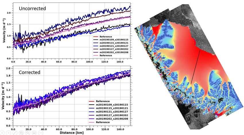
Antarctica_Ice_Sheet_cci+ Reference: ST-UL-ESA-AISCCI+-ATBD-001
 Algorithm Theoretical Basis Document (ATBD) Version : 1.0 page
 for AIS CCI+ Phase 1 Date : 9 March 2020 19/48

3 Ice Velocity
3.1 Introduction
SAR based ice velocity measurements are sensitive to vertical displacements of the reflecting surface due
to the nature of the side looking acquisition geometry (Figure 3.1). If observed from the same point in
orbit, a vertically displaced object , will be detected closer or further away from the sensor since only
the distance in slant range can be detected. The magnitude of the observed slant range displacement
depends additionally on the local incidence angle .

Figure 3.1: Imaging geometry of side looking spaceborne SAR. A vertical displacement of a Point , is
imaged at different slant range position ( ) depending on its elevation.

For floating ice, the major contribution to vertical displacement are:
 • Tides
 Under most ice shelfs surrounding Antarctica the typical peak-to-peak tidal ranges are ~ 1-2 m. At
 spring tides this values can increase to 2-4 m and occasionally can exceed 6 m (Padman et al.,
 2002).
 • Inverted Barometric Effect (IBE)
 During a passage of an energetic polar low a surface pressure change of ~40 hPa results in vertical
 displacement of ~40 cm of sea surface height (Padman et al., 2003). This value is generally
 smaller than the daily mean tide level of ~2 m but larger than the typical tide model error which is
 in the order of 10 cm. Therefore IBE is the second largest contribution to the changing sea surface
 height (Padman et al., 2003).
The presented processing line models these vertical displacements and compensates for the contribution
to the ice velocity. The impact of the tides and IBE is clearly visible in the spread of the ice velocities at
Demorest Glacier, Larsen-C, from Oct. 2015 – Oct. 2017 (Figure 3.2).
The tool is designed to be extendable to newer tide models and reanalysis data/ data sources.
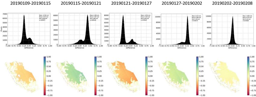
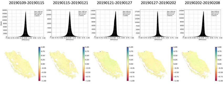
Antarctica_Ice_Sheet_cci+ Reference: ST-UL-ESA-AISCCI+-ATBD-001
 Algorithm Theoretical Basis Document (ATBD) Version : 1.0 page
 for AIS CCI+ Phase 1 Date : 9 March 2020 20/48

Figure 3.2 Sentinel-1 velocity profiles along Demorest Glacier, Larsen-C, from Oct. 2015 – Oct. 2017 clearly
showing the effect of the vertical displacement of the iceshelf, due to tides and atmospheric pressure.

3.2 Review of scientific background
Add justification and importance of tidal correction for ice velocity estimation.
(McMillan et al., 2011) compared three tide models (TPXO7.1, CATS2008a_opt and FES2004) in the
Amundsen Sea with satellite based InSAR measurements from ERS-1/2 and compensated for the tidal
displacement. The selected models perform comparably well with an RMSE of ~9 cm. The further inclusion
of an atmospheric model improved the tide model predictions by 6~%. It was concluded that the applied
correction can compensate for a velocity error of ~22 m/yr in the ground range component of the ice
velocity field. In a similar approach (Wild, Marsh and Rack, 2019) validated satellite based DInSAR
measurements from TerraSAR-X against GPS data collected on Darwin Glacier, draining from the
Transantarctic Mountains to the Ross Sea. The DInSAR measurements were used to improve the tide
model (TPXO7.1) output by up to 39% from 10.8 to 6.7 cm RMSE against GPS at locations where the ice is
in its local hydrostatic equilibrium. For the IBE was accounted.
IBE corrections are justified for atmospheric pressure variations occurring with a frequency of 0.03 to
0.5 cycle per day (Padman et al., 2003) and reduce the standard deviation of the ice-shelf surface
elevation from ~ 9 cm to ~3 cm.
At the transition zones from grounded to floating ice tidal displacement profiles derived from GPS at
Ruthford Ice Stream and Ronne Ice Shelf (Vaughan, 1995) indicated that the flexure can be modelled by
an elastic beam model with a single value for the elastic modulus (0.88±0.35 GPa).

3.3 Algorithms
The processing chain to correct for tide and atmospheric pressure induced ice velocity variations is
illustrated in Figure 3.3. Input to the algorithm are the uncorrected iv-maps in SAR geometry on burst
level, a digital elevation model covering the area of interest, a binary mask identifying the grounded ice as
well as tide models and atmospheric reanalysis datasets. First the tidal difference between the acquisition
dates of the image pair forming the iv-map is modelled, as well as the surface pressure difference. These
model outputs are transformed into SAR geometry. In the second step the elastic beam model (Vaughan,
1995) is applied to the binary mask. Finally, the IV-correction is computed using the geometric relations of
the acquisition geometry depicted in Figure 3.1.
Details on each step performed are described in the following subsections.
Antarctica_Ice_Sheet_cci+ Reference: ST-UL-ESA-AISCCI+-ATBD-001
 Algorithm Theoretical Basis Document (ATBD) Version : 1.0 page
 for AIS CCI+ Phase 1 Date : 9 March 2020 21/48

Figure 3.3 High level processing for compensating ice velocity variations induced by tides and inverse
barometric effect

Note: In the equations bold symbols refer to data arrays in SAR -geometry and vectors ⃗ are marked by
an arrow. Quantities are represented in SI units or derived SI units.

3.3.1 Generation of Groundline Mask
To correct ice velocities of the floating ice and ensure a smooth transition to the grounded ice a proximity
weighted mask is created, following (Vaughan, 1995):

 = ( ) ∙ [ − − ( + )] Equation 3.1

 − ² Equation 3.2
 =
 ³
Where
 • ( ) is the tidal displacement of the ice surface from its mean position here set to 1 m
 • spatial wave number [m-1] incorporating the spatial frequency of the flexure and its decay
 length,
 • is the distance orthogonal to the grounding line in meter
 • is the density of the sea water 1030 kg/m3
 • the gravitational acceleration 9.81 m/s²,
 • is Youngs’s modulus, set to 0.88 GPa,
 • is Poissons’s ratio set to 0.3 and
 • the thickness of the ice shelf approximated with 500 m.
Antarctica_Ice_Sheet_cci+ Reference: ST-UL-ESA-AISCCI+-ATBD-001
 Algorithm Theoretical Basis Document (ATBD) Version : 1.0 page
 for AIS CCI+ Phase 1 Date : 9 March 2020 22/48

The mask reflects the deformation response to tidal forcing. It scales from 0 inland and grounded ice to
1 on open water and floating ice and reaches a maximum value of 1.043 at a distance ~4500 m off the
grounding line (Figure 3.4) with the above stated parameters.
This mask is created once for entire Antarctica in geographic coordinates.

 Figure 3.4: Vertical displacement response of a 500m thick ice shelf to tidal forcing.

3.3.2 Retrieve Geolocation Grid
In order to employ the tide model and IBE corrections the area covered by the SAR image must be
recovered from the slant and azimuth timestamps. This procedure, the forward geocoding, involves a DEM
to extract the latitude longitude geolocation grid (GG) covered by the SAR scene (Small and Schubert,
2019).
This step is performed each SAR iv map.

3.3.3 Compute Local Incidence Angle
The local incidence angle is derived by computing the dot product between unit vector of the line of
sight vector
 ⃗⃗⃗ and the normal vector
 ⃗⃗⃗ to the point of interest in the DEM identified by the GG.

 ⃗⃗ )
 ⃗⃗ ⋅
 = ( Equation 3.3

This step is performed each SAR iv map.

3.3.4 Simulation of differential Tide
To model tides the Python module pyTMD (available at: https://github.com/tsutterley/pyTMD) and tide
OSU (Oregon State University, USA) tide models files (available at https://www.tpxo.net) are utilized.
The GG containing the geographic location of every SAR pixel is passed together with the acquisition
timestamp to the Python module pyTMD toolbox where the tide for the master and the slave acquisition
date is simulated. The tidal prediction is based on Laplace's tidal equations and evaluated with the
following harmonic constituents:
Antarctica_Ice_Sheet_cci+ Reference: ST-UL-ESA-AISCCI+-ATBD-001
 Algorithm Theoretical Basis Document (ATBD) Version : 1.0 page
 for AIS CCI+ Phase 1 Date : 9 March 2020 23/48

 Table 3.1 Selected tidal constituents applied in the Tidal Prediction Software

 Semi-diurnal Symbol
 Principal lunar semidiurnal M2
 Principal solar semidiurnal S2
 Larger lunar elliptic semidiurnal N2
 Lunisolar semidiurnal K2
 Diurnal Symbol
 Lunar diurnal K1
 Lunar diurnal O1
 Solar diurnal P1
 Larger lunar elliptic diurnal Q1
 Long period Symbol
 Lunisolar fortnightly Mf
 Lunar monthly Mm
 Short period (nonlinear) Symbol
 Shallow water overtides of principal lunar M4
 Shallow water quarter diurnal MS4
 Shallow water quarter diurnal MN4

The tidal maps contain the tidal elevations computed with the constituent of Table 3.1 with respect to
the mean sea level (MSL) at a given time. The tidal difference at a position ⃗⃗
 ⃗⃗ (latitude, longitude) is
given by:

 = ( , ⃗
 ⃗⃗) − ( , ⃗
 ⃗⃗) Equation 3.4

Where 0 reflects the acquisition time of the master scene and 1 the acquisition time of the slave scene
forming the image pair for iv retrieval.
This step is performed each SAR iv map.

3.3.5 Simulation of differential Surface pressure

Between two SAR acquisitions and the atmospheric pressure exerted on the ocean surface varies
causing the local sea surface topography to deform which is known as the inverted barometric effect. A
change in 10 hPa in surface air pressure, results in a change of 10 cm at sea level (Equation 3.5). This
vertical displacement causes a range distance change.

 = − − [ / ] Equation 3.5

In order to compensate for the IBE the surface pressure is retrieved from ERA5 Reanalysis dataset. It
contains surface pressure data reanalysed 4-times daily. The surface pressure ( , ⃗⃗
 ⃗⃗) for the acquisition

dates and are linearly interpolated between the adjacent dataset layer at position ⃗⃗
 ⃗⃗ provided in the
GG. For the further processing the surface pressure difference is formed with Equation 3.6.
Antarctica_Ice_Sheet_cci+ Reference: ST-UL-ESA-AISCCI+-ATBD-001
 Algorithm Theoretical Basis Document (ATBD) Version : 1.0 page
 for AIS CCI+ Phase 1 Date : 9 March 2020 24/48

 = ( , ) − ( , ) Equation 3.6

This step is performed each SAR iv map.

3.3.6 Correction of atmospheric and tidal induced iv variations
To the uncorrected ice velocity map a correction term accounting for the tides and the IBE is
added. From vertical tidal displacement (Equation 3.4) the vertical displacement attributed to IBE is
added according to Equation 3.5 and Equation 3.6. The displacement is projected into SAR geometry by
multiplying the product by the cosine of the incidence angle and further dividing it by the slant range
pixel spacing . Applying the mask to the product ensures a smooth transition in ice velocity from
grounded to floating ice. In the last step the displacement is normalized with the time lag between the two
acquisitions to arrive at the ice velocity correction term.

 ( + ) ( )
 = + ( ) Equation 3.7
 ( − )

This step is performed each SAR iv map.

3.4 Input data and algorithm output
The following input data sets are required to run the tidal correction algorithm:
 • Uncorrected iv-map in SAR geometry at burst level
 • Tide Model
 • Mask of grounded ice
 • Reanalysis data of surface pressure
 • Digital Elevation Model (DEM)

3.4.1 Uncorrected iv-map in SAR geometry at burst level
The software takes uncorrected iv maps in SAR geometry on burst level as an input with the ice velocities
given in meters per day. The availability of the state vector information azimuth and slant range timing is
essential to the processing.

3.4.2 Tide Model
The tide model CATS2008: Circum-Antarctic Tidal Simulation version 2008 (CATS2008; Erofeeva et al.,
2019) is a regional ocean tide model. It has a resolution of 4 km within the bounds West: -180, East: 180,
South: -90, North: -40.231. The polar stereographic grid is centred at 71 degrees S, 70 degrees W. The
provided constituents are: M2, S2, N2, K2, K1, O1, P1, Q1, Mf and Mm.
The coastline is based on the MODIS Mosaic of Antarctica (Scambos et al., 2007) feature identification
files, adjusted to match ICESat-derived grounding lines for the Ross and Filchner-Ronne ice shelves and
Interferometric Synthetic Aperture Radar (InSAR) grounding lines.
Satellite altimetry data was used to best-fit the Laplace Tidal Equations in the least squares sense and
obtain the model (Data access: https://www.usap-dc.org/view/dataset/601235).
As CATS2008 has the most accurate grounding line position it was selected for this project.

3.4.3 Mask of Grounded Ice
The basis for the mask ensuring a smooth transition in the ice velocity field is derived from MEaSUREs
Grounding Line dataset (Mouginot, 2017). It comprises grounding line locations between 1992 and 2015
distributed as ESRI shapefiles (Data access: https://nsidc.org/data/nsidc-0709).
You can also read


