Diverging future surface mass balance between the Antarctic ice shelves and grounded ice sheet
←
→
Page content transcription
If your browser does not render page correctly, please read the page content below
The Cryosphere, 15, 1215–1236, 2021
https://doi.org/10.5194/tc-15-1215-2021
© Author(s) 2021. This work is distributed under
the Creative Commons Attribution 4.0 License.

Diverging future surface mass balance between the Antarctic ice
shelves and grounded ice sheet
Christoph Kittel1 , Charles Amory1,2 , Cécile Agosta3 , Nicolas C. Jourdain2 , Stefan Hofer4 , Alison Delhasse1 ,
Sébastien Doutreloup1 , Pierre-Vincent Huot5 , Charlotte Lang1,6 , Thierry Fichefet5 , and Xavier Fettweis1
1 Laboratory of Climatology, Department of Geography, SPHERES research unit, University of Liège, Liège, Belgium
2 Institut
         des Géosciences de l’Environnement (IGE), Univ. Grenoble Alpes/CNRS/IRD/G-INP, Grenoble, France
3 Laboratoire des Sciences du Climat et de l’Environnement, LSCE-IPSL, CEA-CNRS-UVSQ,

Université Paris-Saclay, Gif-sur-Yvette, France
4 Department of Geosciences, University of Oslo, Oslo, Norway
5 Earth and Climate, Earth and Life Institute, Catholic University of Louvain, Louvain-la-Neuve, Belgium
6 National Centre for Atmospheric Science, University of Reading, Reading, United Kingdom

Correspondence: Christoph Kittel (ckittel@uliege.be)

Received: 5 October 2020 – Discussion started: 14 October 2020
Revised: 25 January 2021 – Accepted: 26 January 2021 – Published: 5 March 2021

Abstract. The future surface mass balance (SMB) will influ-       lower mitigation to sea level rise than in ssp585. Over the ice
ence the ice dynamics and the contribution of the Antarctic       shelves, the strong run-off increase associated with higher
ice sheet (AIS) to the sea level rise. Most of recent Antarc-     temperature is projected to decrease the SMB (more strongly
tic SMB projections were based on the fifth phase of the          in CMIP6-ssp585 compared to CMIP5-RCP8.5). Ice shelves
Coupled Model Intercomparison Project (CMIP5). However,           are however predicted to have a close-to-present-equilibrium
new CMIP6 results have revealed a +1.3 ◦ C higher mean            stable SMB under CMIP6 ssp126 and ssp245 scenarios. Fu-
Antarctic near-surface temperature than in CMIP5 at the end       ture uncertainties are mainly due to the sensitivity to anthro-
of the 21st century, enabling estimations of future SMB in        pogenic forcing and the timing of the projected warming.
warmer climates. Here, we investigate the AIS sensitivity to      While ice shelves should remain at a close-to-equilibrium
different warmings with an ensemble of four simulations per-      stable SMB under the Paris Agreement, MAR projects strong
formed with the polar regional climate model Modèle At-           SMB decrease for an Antarctic near-surface warming above
mosphérique Régional (MAR) forced by two CMIP5 and                +2.5 ◦ C compared to 1981–2010 mean temperature, limiting
two CMIP6 models over 1981–2100. Statistical extrapola-           the warming range before potential irreversible damages on
tion enables us to expand our results to the whole CMIP5          the ice shelves. Finally, our results reveal the existence of a
and CMIP6 ensembles. Our results highlight a contrasting          potential threshold (+7.5 ◦ C) that leads to a lower grounded-
effect on the future grounded ice sheet and the ice shelves.      SMB increase. This however has to be confirmed in follow-
The SMB over grounded ice is projected to increase as             ing studies using more extreme or longer future scenarios.
a response to stronger snowfall, only partly offset by en-
hanced meltwater run-off. This leads to a cumulated sea-
level-rise mitigation (i.e. an increase in surface mass) of the
grounded Antarctic surface by 5.1 ± 1.9 cm sea level equiva-      1   Introduction
lent (SLE) in CMIP5-RCP8.5 (Relative Concentration Path-
way 8.5) and 6.3 ± 2.0 cm SLE in CMIP6-ssp585 (Shared             The surface mass balance (SMB) of the Antarctic ice sheet
Socioeconomic Pathways 585). Additionally, the CMIP6              (AIS) is the result of accumulation through snowfall and ab-
low-emission ssp126 and intermediate-emission ssp245 sce-         lation through surface erosion, sublimation, and run-off. Pos-
narios project a stabilized surface mass gain, resulting in a     itive (negative) SMB values reflect a mass gain (loss) at the
                                                                  surface of the ice sheet. The AIS currently loses mass mainly

Published by Copernicus Publications on behalf of the European Geosciences Union.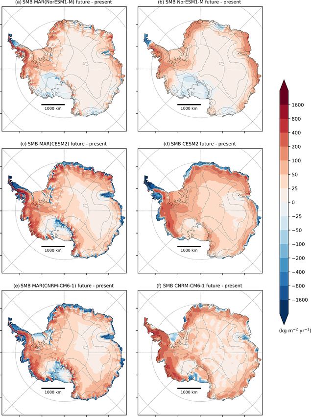
1216                                                       C. Kittel et al.: Future Antarctic surface mass balance using MAR

by ice discharge and basal melting. The difference between          crease (Ligtenberg et al., 2014; Donat-Magnin et al., 2021),
SMB and ice discharge determines the sea-level-rise con-            suggesting an increased risk of hydrofracturing and collapse
tribution of the AIS. Due to the large amount of grounded           (Kuipers Munneke et al., 2014).
ice, the AIS is the largest potential contributor among the            The most recent projections of the Antarctic SMB are
cryosphere (58 m sea level equivalent (SLE); Fretwell et al.,       based on global climate models and earth system models
2013; Morlighem et al., 2020). Although not directly con-           (ESMs) of the fifth phase of the Coupled Model Intercompar-
tributing to sea level variations, relatively flat and large ice    ison Project (CMIP5) (Taylor et al., 2012), whereas new cli-
shelves, i.e. the floating extensions of the ice sheet, never-      mate projections are now available through CMIP6 (O’Neill
theless influence the ice dynamics by restraining the ice over      et al., 2016). Under the highest-emission scenario, projec-
the grounded continent that flows under the force of gravity        tions for the AIS annual mean near-surface temperature in
toward the ocean. This buttressing effect first limits glacier-     2100 are +1.3 ◦ C higher in CMIP6 models than in CMIP5
flow acceleration and then controls ice discharge (e.g. Rignot      models (Fig. 1). However, using these climate model outputs
et al., 2004; Dupont and Alley, 2005; Gudmundsson, 2013;            directly to study the evolution of the SMB often involves sev-
Fürst et al., 2016).                                                eral compromises: (i) their resolution remains too coarse to
   Since the 2000s, the Antarctic ice sheet has been losing         correctly represent the steep margins of the ice sheet or the
mass at an accelerating rate mainly due to an increased ice         peripheral ice shelves (Seroussi et al., 2020), and (ii) they
discharge in the West AIS (Shepherd et al., 2018), itself           do not account properly for important physical processes of
caused by the acceleration of outlet glaciers in response to        polar regions, in particular those related to the stable bound-
basal (ocean) melt thinning the ice shelves and reducing their      ary layer and snow metamorphism, snowmelt, albedo feed-
buttressing effect (Paolo et al., 2015; Gardner et al., 2018;       backs, and refreezing in the snowpack (Lenaerts et al., 2016;
Rignot et al., 2019). Stronger basal melting of ice shelves         Favier et al., 2017). This partly explains why the SMB de-
is further projected to drive future Antarctic mass loss (Hol-      rived from ESMs has often been roughly approximated as
land et al., 2019; Seroussi et al., 2020). Despite stable sur-      precipitation minus evaporation even for projections (e.g.
face melt rates since 1979 (Kuipers Munneke et al., 2012),          Palerme et al., 2017; Favier et al., 2017; Gorte et al., 2019;
atmospheric conditions through intense melt events can lead         Seroussi et al., 2020) or included a run-off computed from
to meltwater ponding at the surface of ice shelves, increas-        non-polar-oriented models (Golledge et al., 2015; Nowicki
ing their potential for hydrofracturing (Scambos et al., 2000;      et al., 2020; Garbe et al., 2020), although a few exceptions
van den Broeke, 2005). The resulting ice shelf collapses over       exist (e.g. Lenaerts et al., 2016; Sellar et al., 2019).
the Antarctic Peninsula then caused enhanced ice discharge             Dynamical downscaling of ESMs (hereafter designating
(Scambos et al., 2004, 2014), highlighting the important role       both global climate models and new-generation earth system
of atmosphere–surface interactions in the AIS stability, likely     models without any consideration of the model sophistica-
to become even more important in the context of global              tion to represent the carbon cycle or cloud–aerosol interac-
warming.                                                            tions) with polar-oriented regional climate models (RCMs)
   With increasing temperatures, more surface mass gain is          offers an alternative not only to address the issue of coarse
expected over the AIS as a result of an increase in pre-            spatial resolution but also more importantly to more robustly
cipitation (Palerme et al., 2017; Gorte et al., 2019). Frieler      evaluate changes in mass and energy fluxes at the ice sheet
et al. (2015) suggested an increase in accumulation linked to       surface (e.g. Fyke et al., 2018; Lenaerts et al., 2019; Fet-
air temperature of ∼ 6 % per degree Celsius, which is con-          tweis et al., 2020). This is why we propose here to use
firmed by SMB reconstructions from ice cores over the 20th          the polar-oriented RCM Modèle Atmosphérique Régional
century (Medley et al., 2018; Medley and Thomas, 2019)              (MAR), widely used over the AIS (e.g. Kittel et al., 2018;
but not retrieved in recent (too short) SMB reconstructions         Agosta et al., 2019; Wille et al., 2019), to downscale an en-
(Van Wessem et al., 2018; Agosta et al., 2019; Mottram et al.,      semble of four different ESMs from the CMIP5 and CMIP6
2020) due to the internal climate variability determining pre-      exercises, selected to cover a wide range of near-surface
cipitation pattern (Previdi and Polvani, 2016). For moder-          warming (+3.2 to +8.5 ◦ C over the Antarctic ice sheet dur-
ate warming, increase in snowfall is likely to outpace in-          ing the 21st century and then statistically extrapolate our re-
creased losses through ablation and especially run-off, mak-        sults to the full CMIP5 and CMIP6 ensembles. This study
ing the Antarctic SMB the only future mitigating contributor        therefore aims to (1) quantify the surface response of the
to sea level rise (Krinner et al., 2007; Agosta et al., 2013;       AIS to warmer climates and more specifically the different
Ligtenberg et al., 2013; Lenaerts et al., 2016; Garbe et al.,       responses of the grounded ice and ice shelves using both
2020). Melt increase under the high-emissions pathway by            new scenarios and an adapted representation of polar pro-
2100 is however projected to be large enough to enhance             cesses; (2) discuss the evolution of individual SMB compo-
ice shelf collapses (Trusel et al., 2015; Donat-Magnin et al.,      nents, including future run-off ablation, that can significantly
2021). The future of ice shelves experiencing more snow-            compensate for mass gained through snowfall; and (3) as-
fall, which can enable the snowpack to absorb more liquid           sess the future contribution (and related uncertainties) of the
water, is still uncertain even if the firn air content should de-   grounded Antarctic SMB to sea level rise and the future state

The Cryosphere, 15, 1215–1236, 2021                                                    https://doi.org/10.5194/tc-15-1215-2021
C. Kittel et al.: Future Antarctic surface mass balance using MAR                                                                 1217

Figure 1. Time series of the 90–60◦ S annual near-surface temperature anomaly (◦ C) compared to the present reference period (1981–2010)
from the ERA5 reanalysis and ESMs using the extreme high-emission scenarios the Relative Concentration Pathway 8.5 (RCP8.5) and
Shared Socioeconomic Pathways 585 (ssp585) after their historical period (2004 for CMIP5 and 2014 for CMIP6). The thick blue and red
lines represent the mean annual warming from 28 CMIP5 and 34 CMIP6 ESMs. Thinner orange and blue lines are for ESMs selected as
boundary conditions for our regional climate model MAR: CNRM-CM6-1 and CESM2 (CMIP6, ssp585) and NorESM1-M and ACCESS1-3
(CMIP5, RCP8.5). The dashed black line is the ERA5 reanalysis (1960–2020) (Hersbach et al., 2020).

of the peripheral ice shelves using all the CMIP5 and new             and/or ice. SISVAT solves the surface energy budget using
CMIP6 models with different emissions scenarios by extrap-            excess in energy to melt the snow. Each snow and/or firn
olating RCM-derived SMB projections.                                  layer has a maximum water retention of 5 %, while the re-
                                                                      maining liquid water – coming from rainfall or surface melt-
                                                                      water – can freely percolate downward as long as the un-
2     Methods                                                         derlying snow density does not reach a close-off density of
                                                                      830 kg m−3 . Remaining liquid water beyond the snowpack
2.1    The regional atmospheric model MAR                             saturation is converted into surface run-off, meaning that in
                                                                      the absence of a water-routing hydrologic scheme, all surface
MAR is a polar-oriented regional climate model frequently             water that could potentially form melt ponds is considered to
used to study the Antarctic (e.g. Amory et al., 2015; Kittel          be run-off, i.e. is lost by the ice sheet. Snow and/or ice surface
et al., 2018; Agosta et al., 2019) and Greenland (e.g. Fet-           albedo varies as a function of the optical properties of snow,
tweis et al., 2017; Hofer et al., 2017; Delhasse et al., 2019)        the presence of bare ice or liquid water, the snow depth over
ice sheet climates. MAR is a hydrostatic model relying on the         ice, and clouds (Tedesco et al., 2016), with a maximum value
primitive equations described in Gallée and Schayes (1994).           of 0.94 for fresh snow and a minimum value of 0.55 for bare
The model includes a cloud microphysics module solving                ice over Antarctica.
conservation equations for five water species: snow parti-               In this study, we used the latest MAR version (3.11), in this
cles, cloud ice crystals, rain drops, cloud droplets, and spe-        paper referred to as MAR. The latest updates in MAR im-
cific humidity (Gallée, 1995). Airborne particles can be ad-          prove the cloud lifetime, the model stability, and its compu-
vected vertically from one atmospheric layer to another and           tational efficiency and reduce the dependency on the model
notably contribute through sublimation to the heat and mois-          time step. Several other improvements have also been made
ture budget of the atmosphere (Agosta et al., 2019). The              in MAR relative to the previous model versions used over
radiative transfer scheme is adapted from European Centre             Antarctica (Agosta et al., 2019) and are detailed below.
for Medium-Range Weather Forecasts (ECMWF) ERA-40
reanalysis (Morcrette, 2002). The transfer of mass and en-
ergy between the surface and the atmosphere is simulated in             a. Inclusion of rock outcrops in the ice sheet mask, en-
the 1-D surface scheme SISVAT (Soil Ice Snow Vegetation                    abling potential feedbacks between low-albedo exposed
Atmosphere Transfer; De Ridder and Gallée, 1998) mod-                      rocks (0.17 in MAR) and enhanced snow melting (e.g.
ule, which consists of soil and vegetation (De Ridder and                  Kingslake et al., 2017) around pixels partially com-
Schayes, 1997), snow (Gallée and Duynkerke, 1997; Gallée                   posed of rocks: this also resulted in the ice mask be-
et al., 2001), and ice (Lefebre et al., 2003) sub-modules. The             ing enlarged at the margins while reducing the ice sheet
latter two are originally based on the snow model CROCUS                   area. SISVAT computes the different exchanges for the
(Brun et al., 1992). The dynamical snow and ice compo-                     rock surface separately from the snow-,firn, and/or ice-
nents represent snow properties and metamorphism across 30                 covered part and then weight-aggregates them accord-
snow, firn, and/or ice layers, resolving the first 20 m of snow            ing to the proportion of each sub-grid cell.

https://doi.org/10.5194/tc-15-1215-2021                                                      The Cryosphere, 15, 1215–1236, 2021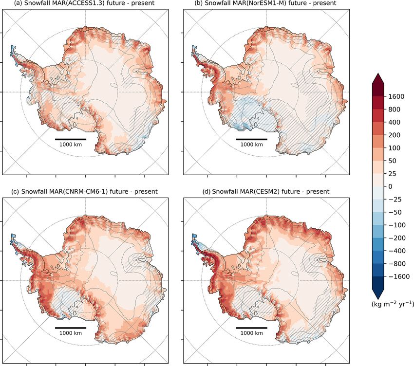
1218                                                        C. Kittel et al.: Future Antarctic surface mass balance using MAR

  b. Addition of a vertical atmospheric level (from 23 to 24)        +8.5 W m−2 by 2100 but differ in how the anthropogenic
     for a CPU-allocation reason (better parallelization along       forcing is split between individual drivers of global warming
     the vertical axis): note that MAR near-surface results          (O’Neill et al., 2016).
     are not sensitive to the additions of more atmospheric             The selection of ESMs that were dynamically downscaled
     levels (Amory et al., 2020).                                    by MAR was based on their ability to (i) represent the cur-
                                                                     rent climate (air temperature and humidity, sea surface condi-
  c. Modification of the fresh falling snow density, now             tions, and large-scale circulation) around the AIS and (ii) di-
     computed as a function of the 10 m wind speed ws10              versify the projected changes during the 21st century. These
     (m s−1 ) only:                                                  criteria ensure on the one hand, that the ESM biases will not
                                                                     have a prejudicial effect on the projections since the present
     ρs = 200 + 32 ws10 ,                                     (1)    state determines future biases (Agosta et al., 2015; Krinner
                                                                     and Flanner, 2018) and on the other hand that we assess the
     with minimum and maximum values fixed to 300 and
                                                                     AIS response to a wide range of projected temperature in-
     400 kg m−3 in accordance with observations (Table S2
                                                                     creases for a better quantification of the future uncertainties
     in Agosta et al., 2019) and the new developments into
                                                                     for a same scenario. We therefore firstly ranked ESMs by
     the drifting-snow scheme (Amory et al., 2020).
                                                                     comparing them to the ECMWF reanalysis ERA5 (Hersbach
   The Antarctic topography and ice and rock fraction are            et al., 2020) over the recent “historical” period (1980–2004)
computed from the 1 km resolution digital elevation model            following the method defined in Agosta et al. (2015) and
Bedmap2 (Fretwell et al., 2013). The ice mask is fixed and           Barthel et al. (2020) for CMIP5, extended here to CMIP6 and
cannot evolve, meaning that changes in ice extent follow-            applied only to the Antarctic atmosphere. The method firstly
ing for instance an ice shelf collapse are not represented.          computes the root mean square error (RMSE) compared to
The same is true for surface elevation, which is assumed to          ERA5 for several climate variables (mean air temperature at
remain constant in the absence of ice dynamics and evolv-            850 hPa, annual precipitable water, annual sea level pressure,
ing topography. Therefore, feedbacks between the ice sheet           summer sea surface temperature, and winter sea ice extent
geometry and the atmosphere are not taken into account in            over 1980–2004) that are supposed to determine the SMB
our simulations. Finally, as the drifting-snow scheme (Amory         (Agosta et al., 2015). The score of each ESM is then ob-
et al., 2020) was still under development when we performed          tained by averaging its RMSEs that were previously normal-
our simulations, it was not activated in this study.                 ized with regards to the multi-model median and interquartile
                                                                     range. This enables the combination of several metrics using
2.1.1   Selection of ESMs                                            the same weight for each of the metrics. Once the models
                                                                     were ranked on the basis of their score against ERA5, the fi-
Large-scale forcing models were chosen among the CMIP5               nal selection was made to diversify the changes expected at
and CMIP6 ESMs. CMIP6 models rely on an improved and                 the end of the century and the availability of 6-hourly outputs
more sophisticated representation of the global climate sys-         in the CMIP5 and CMIP6 database at the end of 2019, when
tem than CMIP5. They incorporate better coupling between             we started our experiments.
the different components of the earth system and improved               We selected two models from the CMIP5 ensemble, AC-
present and better-constrained future concentration scenarios        CESS1.3 and NorESM-M, and two from CMIP6, CNRM-
of long-lived greenhouse gases and aerosols (Eyring et al.,          CM6-1 and CESM2. The Antarctic (90–60◦ S) near-surface
2016; O’Neill et al., 2016). Additionally, most CMIP6 ESMs           warming they produce for RCP8.5 (CMIP5) and ssp585
are also run at a higher spatial resolution. First analyses of the   (CMIP6) is shown in Fig. 1. Figure 1 also illustrates that
CMIP6 results revealed higher equilibrium climate sensitiv-          ESMs correctly reproduce the mean warming since 1960.
ity in this new generation of models (Mauritsen et al., 2019;        ACCESS1.3 (Bi et al., 2013; Dix et al., 2013) is the model
Voldoire et al., 2019; Zelinka et al., 2020; Meehl et al., 2020;     that best represents the present Antarctic climate compared to
Wyser et al., 2020), suggesting warmer future climates while         ERA-Interim (Agosta et al., 2015), and it is also among the
based on similar future scenarios in terms of global radia-          best models when compared to ERA5 (Agosta et al., 2021).
tive forcing. However, this higher climate sensitivity is po-        This ESM has a near-surface Antarctic warming close to the
tentially not supported by palaeo-climate records (Zhu et al.,       CMIP6 multi-model mean (+5 ◦ C). NorESM1-M (Bentsen
2020). We therefore also included models from the CMIP5              et al., 2013; Iversen et al., 2013) projects a weaker Antarctic
dataset, some of which show a good comparison with re-               atmospheric warming (+3.2 ◦ C; Fig. 1) but a stronger ocean
analyses over the current Antarctic climate (Agosta et al.,          warming (Barthel et al., 2020). CNRM-CM6-1 (Voldoire
2015; Palerme et al., 2017). We only chose the scenarios of          et al., 2019) correctly represents the present Antarctic cli-
the largest greenhouse gas emissions from CMIP5 (RCP8.5)             mate and was among the first models available in the CMIP6
and its updated version in CMIP6 (ssp585) in order to obtain         database. This model also enables the assessment of the AIS
stronger warming signals and then SMB sensitivities. These           response to an extreme Antarctic warming (+8.5 ◦ C) since it
two scenarios have an equivalent global radiative forcing of         is the warmest model over the AIS among the CMIP5 and

The Cryosphere, 15, 1215–1236, 2021                                                     https://doi.org/10.5194/tc-15-1215-2021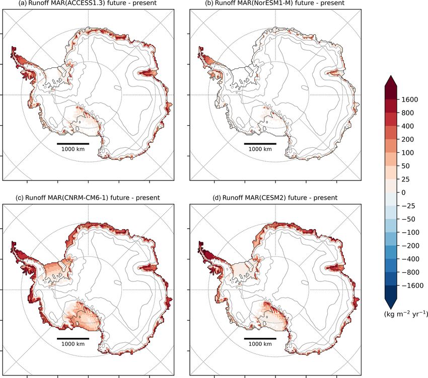
C. Kittel et al.: Future Antarctic surface mass balance using MAR                                                            1219

CMIP6 databases at the end of the 21st century. CESM2              rent climate, but raw values over the grounded ice sheet and
(Danabasoglu et al., 2020) has a lower score than half of the      ice shelves are available in the Supplement (Table S3).
CMIP5 and CMIP6 models compared to ERA5 (Agosta et
al., 2021). Despite its modest ranking, it was chosen due to its
relatively detailed representation of polar oriented processes,    3   Evaluation of MAR(ESM) simulations of the present
early availability, and the frequent use of this model and its
earlier version to study the AIS (e.g. Lenaerts et al., 2016;      Present biases might have a significant influence on the pro-
Fyke et al., 2017; Medley et al., 2018; Nowicki et al., 2020).     jection results and remain in the future (Fettweis et al., 2013;
Its projected warming (+7.7 ◦ C) is close to the mean warm-        Agosta et al., 2015; Krinner and Flanner, 2018; Fettweis
ing projected by CNRM-CM6-1. From this perspective, se-            et al., 2020), highlighting the need for a thorough evaluation
lecting both CESM2 and CNRM-CM6-1 does not maximize                over the present climate. Since ESMs only simulate meteo-
the warming range covered and prevents our selected ESM            rological conditions representative of a certain climate, eval-
ensemble from being representative of the mean CMIP5 and           uating MAR ESM-forced simulations cannot be done using
CMIP6 warming. Yet, it enables us to assess the AIS re-            the observations directly. We then compared these simula-
sponse (and uncertainties) related to the strong warming that      tions to the averaged MAR(ERA5), hereafter considered as a
is only projected by a few ESMs.                                   reference and evaluated in Sect. S1.
                                                                      MAR(ACCESS1.3) is the experiment that best compares
                                                                   with the reference MAR(ERA5) over the present climate.
2.1.2   Experiments
                                                                   It displays the lowest integrated-SMB anomaly (Table S2)
                                                                   and spatial RMSE and bias (Fig. 2). MAR(ACCESS1.3) un-
MAR is forced by 6-hourly large-scale forcing fields at its        derestimates SMB over Wilkes Land, Queen Mary Land,
atmospheric lateral boundaries (pressure, wind, specific hu-       and the Amundsen sector, while it overestimates SMB over
midity, and temperature), at its sea surface (sea ice concen-      Queen Maud Land and the lee side of the Antarctic Penin-
tration and sea surface temperature), and at the top of the        sula. These negative anomalies are associated with the small
troposphere (wind and temperature). We forced MAR with             underestimation of the summer and winter precipitable wa-
the selected ESMs over 1976–2100 (Sect. 2.1.1), and the            ter in ACCESS1.3 (Agosta et al., 2015). This experiment also
first 5 years (1976–1980) were discarded as spin-up. The           reveals mostly non-significant temperature biases in summer
simulations are called MAR(ACCESS1.3), MAR(CESM2),                 (Fig. S3), except for a small negative bias over Ross and
MAR(CNRM-CM6-1), and MAR(NorESM1-M) hereafter.                     Rhone ice shelves, yielding very similar integrated melt val-
We used the same intermediate spatial resolution (35 km)           ues.
as in Agosta et al. (2019) and Mottram et al. (2020) as a             MAR(NorESM1-M) presents mostly non-significant
computation time compromise to run the model with mul-             anomalies compared to MAR(ERA5) but overestimates
tiple forcings over the 20th and the 21st centuries. In or-        the mean integrated annual SMB as a consequence of an
der to assess the quality of the downscaling over the present      overestimation of the snowfall and, to a lesser extent, a
climate, we also forced MARv3.11 by the ERA5 reanaly-              lower surface ablation (Table S2). Higher snowfall values
sis (MAR(ERA5) hereafter). This comparison between MAR             are modelled over Marie Byrd Land, the peninsula, and
forced by the different ESMs as well as an evaluation of           the Brunt Ice Shelf, while lower values compensate this
MAR(ERA5) is available as a Supplement. It shows that              overestimation over Queen Mary Land, Wilkes Land, and
MAR(ERA5) performs similarly to MARv3.10 forced by                 the Amery Ice Shelf (Fig. S4), which are strongly linked
ERA-Interim, which was among the best simulations in               with the humidity anomalies in the forcing ESM (Agosta
terms of both present Antarctic near-surface climate and           et al., 2015). NorESM1-M being too cold (with lower
SMB in the recent evaluation conducted by Mottram et al.           free-atmosphere summer and ocean temperatures as well as
(2020). We refer to Supplement S1 for more details about the       higher sea ice concentration), MAR(NorESM1-M) displays
comparison and evaluation of MARv3.11 in terms of near-            a negative temperature anomaly up to 3 ◦ C over the plateau
surface climate, melt, and SMB.                                    despite reducing the negative anomaly over half of the
   In this study, we have chosen to define the reference pe-       Antarctic ice sheet to non-significant differences in summer
riod of the present climate as 1981–2010. This 30-year refer-      (Fig. S3). This however leads to reduced surface melting
ence period coincides with the availability of reanalyses and      (−72 Gt yr−1 ).
is a compromise between the end of the historical scenar-             MAR(CNRM-CM6-1) simulates nearly the same inte-
ios, which last until 2004 for CMIP5 and 2014 for CMIP6.           grated snowfall amount as MAR(ERA5) but has a higher
Furthermore, Mottram et al. (2020) showed that this period         SMB RMSE due to a less accurate spatial representation of
is characterized by a relatively stable SMB over Antarctica.       the precipitation. This results from an overestimation of the
Projected SMB and component values are given compared              precipitable water combined with a higher mean sea level
to their respective mean values over current climate to re-        pressure in CNRM-CM6-1, potentially reducing cyclonic ac-
move the dependence of the potential linear biases over cur-       tivity. MAR(CNRM-CM6-1) underestimates the SMB over

https://doi.org/10.5194/tc-15-1215-2021                                                 The Cryosphere, 15, 1215–1236, 2021
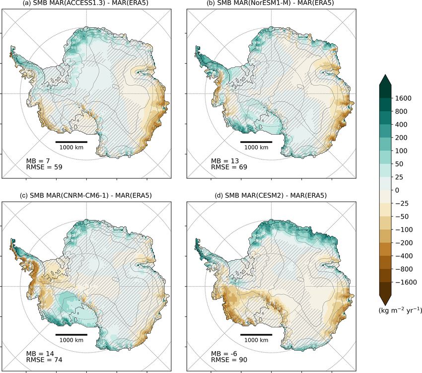
1220                                                          C. Kittel et al.: Future Antarctic surface mass balance using MAR

Figure 2. Comparison between the annual mean SMB simulated by MAR forced by ACCESS1.3 (a), NorESM1-M (b), CNRM-CM6-1
(c), and CESM2 (d) and the annual mean SMB simulated by MAR(ERA5) (kg m−2 yr−1 ) over 1981–2010. Locations where anomalies are
smaller than the (natural) interannual variability in the present climate (interannual standard deviation) are hatched. Mean bias (MB) and root
mean square error (RMSE) compared to MAR (ERA5) are also indicated (units: kg m−2 yr−1 ).

Ellsworth Land and the windward side of the peninsula but                 in the SMB over the historical period. MAR(ACCESS1.3)
overestimates it over Marie Byrd Land, Queen Maud Land,                   has the best representation of the Antarctic SMB over
and Victoria Land (Fig. 2). Agosta et al. (2021) revealed                 the current climate (mean bias: −3 Gt yr−1 ; spatial RMSE:
a strong negative temperature anomaly surrounding the ice                 59 kg m−2 yr−1 ), while MAR(CESM2) is the least accurate
sheet, yielding a lower temperature in MAR(CNRM-CM6-1)                    (mean bias: −26 Gt yr−1 ; spatial RMSE: 90 kg m−2 yr−1 ).
compared to MAR(ERA5) over the plateau. However, these                    The results of our experiments over the current climate are
differences are non-significant over the margins, the Ronne               consistent with the ranking of the ESMs given by Agosta
Ice Shelf excepted (Fig. S3).                                             et al. (2015), Barthel et al. (2020), and Agosta et al. (2021).
   As it simulates lower snowfall amounts than                            This highlights the importance of selecting ESMs that cor-
MAR(ERA5), MAR(CESM2) slightly underestimates                             rectly represent the historical climate (in particular the free
the mean integrated SMB. However, MAR(CESM2) rep-                         atmosphere and the general circulation) around Antarctica as
resents a stronger accumulation over the area between the                 they induce biases in the downscaled near-surface climate in-
peninsula, Queen Maud Land, and Enderby Land (Fig. 2).                    dependently of the capacity of the RCM to improve ESM
This results from the significant overestimation of the                   results. It is also important to note that the spatial and inte-
precipitable water and the sea level pressure in CESM2                    grated anomalies are close to (or even lower than) the spread
over this area. In contrast, MAR(CESM2) simulates a                       between several RCMs, all forced by ERA-Interim (Mottram
lower accumulation over Wilkes Land and the Amundsen                      et al., 2020). This suggests a good ability of the different sim-
sector. CESM2 is colder than ERA5, but the difference is                  ulations to closely reproduce the SMB over the present cli-
reduced in summer (Agosta et al., 2021), leading to mostly                mate and gives some confidence in the results of the future
non-significant temperature anomalies in summer (Fig. S3).                projections.
   In general, the SMB downscaled by MAR forced by the
four ESMs is close to MAR(ERA5). The anomalies of the
annual mean SMB are lower than the interannual variability

The Cryosphere, 15, 1215–1236, 2021                                                            https://doi.org/10.5194/tc-15-1215-2021
C. Kittel et al.: Future Antarctic surface mass balance using MAR 1221
4 Results end of the 21st century. Finally, only MAR(CNRM-CM6-1)
suggests an SMB decrease beyond 2095.
Our projections of the Antarctic SMB show a trend to- The grounded-SMB trend is mainly dominated by an in-
wards surface mass gains by the end of the 21st cen- crease in snowfall (Fig. 5b). Increased air moisture content
tury (Fig. S5). MAR simulations forced by the high- associated with higher air temperatures leads to a widespread
emission scenarios ssp585 and RCP8.5 suggest a gener- increase in snowfall over the AIS, explaining most of the
ally higher Antarctic SMB (including ice shelves) dur- positive SMB anomalies. This increase is stronger where
ing 2071–2100 than for 1981–2010, with positive anoma- air masses saturate as they adiabatically cool when rising
lies between +257 Gt yr−1 for MAR(CNRM-CM6-1) and with the topography (Agosta et al., 2013; Ligtenberg et al.,
+505 Gt yr−1 for MAR(CESM2). The projections reveal a 2013). Figure 4 shows that the largest increase occurs in
spread of 248 Gt yr−1 , i.e. almost a factor of 2 between the West Antarctica, where the accumulation by snowfall is al-
lowest and the highest increase in SMB. Such a high ampli- ready the highest in the present climate. Although more
tude highlights the importance of using multiple models for snowfall can be expected over most of the AIS in a warmer
a better assessment of the uncertainties when discussing the climate (Palerme et al., 2017), some parts of the Antarctic
future state of the Antarctic SMB throughout the 21st cen- grounded ice sheet show negative anomalies. This decrease
tury. in snowfall affects areas such as inland of Marie Byrd, where
the SMB consequently decreases. This strong snowfall in-
4.1 Regional changes crease over the peripheral slopes associated afterwards with
an inland reduction could result from enhanced condensa-
tion over the marginal slopes, reducing moisture intrusion
Using Antarctic-integrated values however hides two distinct
and snowfall formation inland (Kittel et al., 2018). Although
signals. The diverging trajectories of SMB over grounded
this effect may be present in our projections, Fig. S7b also
versus floating ice (Fig. 3) suggest contrasting processes
reveals a deepening of the Amundsen Sea Low, enhanc-
at play. In the rest of this paper, we therefore discuss the
ing moisture advection towards the Antarctic peninsula in
ice shelves and the grounded ice sheet separately. This dis- MAR(NorESM1-M). This deepening projected by NorESM-
tinction is also justified by the direct equivalent between M especially occurs in winter (Raphael et al., 2016) and re-
grounded-ice mass change and mean sea level variations,
sults from rising greenhouse gas emissions (Hosking et al.,
whereas ice shelves do not directly contribute to sea level
2016; Raphael et al., 2016).
variations even if their surface processes (such as hydrofrac-
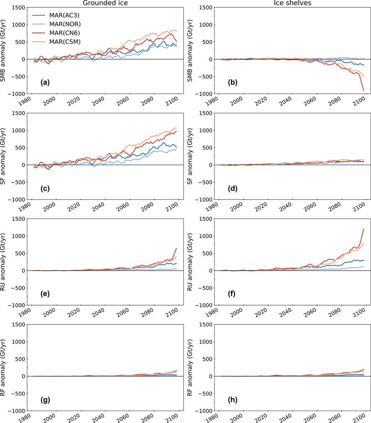
Snowfall increase in response to higher air temperatures
turing) are of crucial importance for the ice sheet dynamics
also competes with a subsequent increase in run-off over the
and therefore the Antarctic mass balance evolution. The lo- grounded ice margins (Fig. 5e). Although run-off amounts
cations mentioned hereafter are illustrated in Fig. S6. are negligible in the present climate, and the increase in run-
off is lower than the increase in snowfall, the future run-off
4.1.1 Grounded ice sheet contribution could compensate up to 34 % of the snowfall in-
crease in MAR(CNRM-CM6-1) over 2071–2100, question-
The grounded Antarctic SMB is projected to increase ing the use of precipitation–evaporation to compute SMB in
by +349 Gt yr−1 (MAR(NorESM1-M)) to +751 Gt yr−1 earlier studies (e.g. Palerme et al., 2017; Favier et al., 2017;
(MAR(CESM2)) from 1981–2010 to 2071–2100 (Table 1). Gorte et al., 2019). Other surface mass flux components such
Our simulations suggest large (up to more than twice the as rainfall (Fig. 5g), deposition, and sublimation are not pro-
present – natural – interannual variability) positive SMB jected to contribute significantly to SMB changes.
anomalies in West Antarctica (Marie Byrd and Ellsworth From 1981 to 2100, our results suggest a grounded cumu-
Land) and over the mountainous regions of the Antarctic lative contribution of −3.7, −5.8, −8.1, and −10.6 cm
Peninsula (Fig. 3). The situation in East Antarctica is more SLE for MAR(NorESM1-M), MAR(ACCESS1.3),
contrasted. The increase is significant (i.e. larger than the in- MAR(CNRM-CM6-1), and MAR(CESM2), respectively.
terannual variability over 1981–2010) in Queen Mary Land Given that all these projections are obtained from similar
and high-elevation plateaus, while George V Land, Adélie anthropogenic forcings, this demonstrates the necessity of
Land, and Wilkes Land are projected to have a weak increase using several ESMs to evaluate the Antarctic contribution to
in SMB for all the simulations, except MAR(CNRM-CM6- the sea level rise in high-emission scenarios at the end of the
1), which suggests a strong increase there. 21st century.
From 2015 onwards, the grounded SMB increases in all
our MAR simulations (Fig. 5a). Large differences between 4.1.2 Ice shelves
projections appear around 2040–2050, when MAR(CESM2)
and MAR(CNRM-CM6-1) suggest the strongest increase af- The SMB evolution over the ice shelves shows more un-
ter 2050 and 2065, respectively, while MAR(NorESM1-M) certainties depending on the forcing ESM. It remains close
and MAR(ACCESS1.3) show a substantial increase at the to the present-day values in MAR(NorESM1-M), while
https://doi.org/10.5194/tc-15-1215-2021 The Cryosphere, 15, 1215–1236, 2021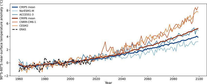
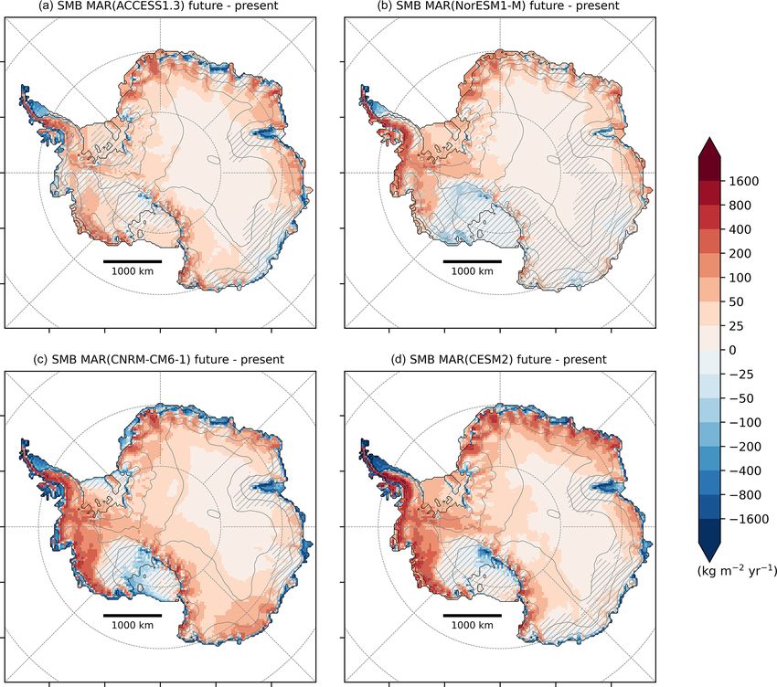
1222                                                      C. Kittel et al.: Future Antarctic surface mass balance using MAR

Figure 3. SMB changes (kg m−2 yr−1 ) between 2071–2100 and 1981–2010 as modelled by MAR forced by ACCESS1-3 (a), NorESM1-
M (b), CNRM-CM6-1 (c), and CESM2 (d). Locations where future changes are smaller than the (natural) interannual variability over the
present climate (interannual standard deviation) are hatched.

Figure 4. Snowfall changes (kg m−2 yr−1 ) between 2071–2100 and 1981–2010 as modelled by MAR forced by ACCESS1-3 (a), NorESM1-
M (b), CNRM-CM6-1 (c), and CESM2 (d) using ssp585 and RCP8.5. Locations where changes are smaller than the (natural) interannual
variability in the present climate (interannual standard deviation) are hatched.

The Cryosphere, 15, 1215–1236, 2021                                                     https://doi.org/10.5194/tc-15-1215-2021
C. Kittel et al.: Future Antarctic surface mass balance using MAR                                                                     1223

Figure 5. Time series of the integrated annual SMB (a, b), snowfall (SF) (c, d), run-off (RU) (e, f), and rainfall (RF) (g, h) anomalies
(Gt yr−1 ) over the Antarctic grounded ice (a, c, e, g) and the Antarctic ice shelves (b, d, f, h) from 1980 to 2100 simulated by MAR forced
by RCP8.5 or ssp585 scenarios from ACCESS1-3 (blue), NorESM1-M (light blue), CNRM-CM6-1 (red), and CESM2 (orange) compared
to the 1981–2010 reference period. A running average of 5 years was applied to the original time series for better readability. Sublimation
and surface melt changes are shown in Fig. S8.

it strongly decreases after 2075 in the other simulations               and negative in MAR(CNRM-CM6-1) and MAR(NorESM1-
(Fig. 5b). All the MAR simulations agree on a significant               M). The Ross Ice Shelf illustrates the large uncertainties re-
SMB decrease over the ice shelves on the lee (eastern) side of          lated to the different model forcings on the future SMB over
the northern Antarctic Peninsula and near Amery’s ground-               the Antarctic ice shelves until 2100.
ing line (Fig. 3). With the exception of MAR(NorESM1-                      MAR suggests an increase in snowfall over ice shelves
M), our projections also suggest a strong SMB decrease                  (between +83 and +139 Gt yr−1 ) regardless of the forc-
over the ice shelves on the windward side of the northern               ing ESM but also a significant increase in rainfall (+18 to
peninsula and over a majority of the ice shelves in Wilkes              108 Gt yr−1 ) (Table 1). The increase in snowfall over the
Land and in Queen Maud Land. Only MAR(CNRM-CM6-                         ice shelves is however weaker than the increase over the
1) reveals widespread negative SMB anomalies over all the               grounded margins, suggesting a stronger saturation of air
small Antarctic peripheral ice shelves. The Ronne–Filchner              masses when lifted over the ice sheet slope (Fig. 4). Over
Ice Shelf is expected to have an increase in SMB, even in               the period 2071–2100, rainfall anomalies can be as large as
MAR(CNRM-CM6-1), except in the vicinity of the ocean.                   snowfall anomalies on the ice shelves or even outpace the
Our simulations suggest diverging responses over the Ross               increase in snowfall in MAR(CNRM-CM6-1), where snow-
Ice Shelf, positive in MAR(ACCESS1.3) and MAR(CESM2)                    fall is projected to decrease at the very end of the century

https://doi.org/10.5194/tc-15-1215-2021                                                        The Cryosphere, 15, 1215–1236, 2021
1224 C. Kittel et al.: Future Antarctic surface mass balance using MAR
(Fig. 5h). The warmer air also induces a conversion of snow- anomalies over 90–60◦ S from the forcing ESM. Figure 7
fall into rainfall over the Antarctic Peninsula, where the to- reveals more consistent projections between all our exper-
tal precipitation is projected to increase despite an increasing iments. Note that associating annual MAR anomalies with
fraction falling as rain. Snowfall also decreases over the Ross ESM temperature anomalies in the free atmosphere (700 or
Ice Shelf in MAR(NorESM1-M) due to a pronounced inten- 850 hPa) does not change the comparison (not shown).
sification of the Amundsen Sea Low system bringing more Precipitation increases following the Clausius–Clapeyron
moisture towards the peninsula and less over the Ross Ice relation, a weak exponential form that can be approximated
Shelf (Fig. S7b), which reduces SMB over this area. as a (nearly) linear relationship for moderate warming over
Higher air temperature also causes a significant increase the AIS (Agosta et al., 2013; Frieler et al., 2015; Palerme
in surface melt. Repeated years of intense melting, combined et al., 2017). The grounded (Fig. S10a) increase is dominated
with increased rainfall, reduce the firn air content and weaken by snowfall anomalies (Fig. 7a) with a weak contribution of
the snowpack capacity to retain liquid water. This results in rainfall (Fig. 7c). Over the ice shelves, snowfall is no longer
large run-off production rates over the ice shelves, except increasing for strong warmings above +7.5 ◦ C. As the total
over the Ronne–Filchner due to its more southern position, as increase in precipitation also remains approximately linear
displayed in Fig. 6. MAR(NorESM1-M) suggests the lowest (Fig. S10b), an increasing proportion of the potential addi-
increase in run-off (+18 Gt yr−1 ), which is 1 order of magni- tional precipitation falls as rain instead of snow for higher
tude lower than for MAR(CNRM-CM6-1) (+558 Gt yr−1 ). temperatures over the ice shelves. Under increasing warm-
The amount of run-off projected at the end of the cen- ing, more locations will experience rainfall, melting, and run-
tury explains the large changes in SMB over the ice shelves off. We therefore link rainfall (Fig. 7c, d) and run-off (Fig. 7e,
(Fig. 5f). The projected SMB decrease in MAR(CNRM- f) anomalies with near-surface temperature anomalies using
CM6-1) over the Ross Ice Shelf results from the larger in- a quadratic relation reflecting positive feedbacks (Fettweis
crease in run-off than in snowfall, while the decrease in SMB et al., 2013). Our results suggest that the increase in rain-
in the MAR(NorESM1-M) experiment is only attributed to fall will be stronger than the snowfall increase over the ice
reduced snowfall accumulation. Finally, the sharp run-off in- shelves for warming above +7.5 ◦ C. The integrated increase
crease in MAR(CNRM-CM6-1) starting in 2090 reflects a in run-off is stronger over ice shelves than over the grounded
widespread run-off over nearly all the ice shelves (Fig. 6). ice, despite lower floating areas. This is mainly explained
by the low surface elevation of the ice shelves. Other stud-
4.2 Links with the ESM near-surface temperature ies (e.g. Kuipers Munneke et al., 2014; Trusel et al., 2015;
Donat-Magnin et al., 2021) also linked an exponential in-
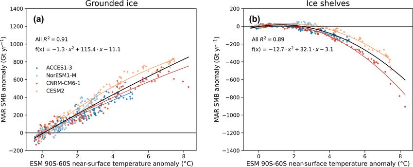
Our projections of the 21st-century evolution of the Antarc- crease in melting with air temperature over the AIS.
tic SMB yield a large spread in SMB for both the Antarc- Although the dominant signal explaining grounded-SMB
tic grounded ice and ice shelves. This spread can mostly be variations is the snowfall increase, the trend suggest a slow-
attributed to different warming rates in the forcing ESM as ing or even a lower grounded-SMB increase for warm-
they show a broad range of warming rates despite a similar ings higher than +7.5 ◦ C (Fig. 8). This results from a
radiative forcing due to anthropogenic emissions (Fig. 1). strong increase in the grounded-ice-sheet run-off. How-
We identify the 30-year periods (different for each ESM) ever, this grounded-SMB threshold is only supported by
characterized by an Antarctic (90–60◦ S) annual near-surface MAR(CNRM-CM6-1). Since this warming magnitude is not
climate about +2.5 ◦ C warmer on average than the cli- reached across all our other projections and as CNRM-CM6-
mate over the historical period (1981–2010) to compare 1 is the warmest model in the entire CMIP5 and CMIP6
SMB anomalies resulting from an equivalent warming. This database, it would require longer projections to confirm the
+2.5 ◦ C warming corresponds to the strongest 30-year- confidence of this threshold.
averaged near-surface warming common to all our selected Over the ice shelves, a near-surface temperature increase
ESMs. The period selected for each ESM is listed in Ta- by more than +2 ◦ C results in run-off anomalies larger
ble S4. Mean SMB anomalies projected by MAR during than precipitation anomalies, hence leading to negative SMB
these periods reveal a very similar spatial pattern between all anomalies (Fig. 8). While ice shelf collapses could already
our experiments. A +2.5 ◦ C warming yields a mostly non- occur due to hydrofracturing caused by enhanced surface
significant increase in SMB over the grounded ice sheet and melt, additional warming beyond this threshold will result
a weak (negative) change over the surrounding ice shelves in less surface accumulation or even ice shelf thinning for
(Fig. S9). This comparison at equivalent warming but differ- the warmings that result in an SMB decrease stronger than
ent 30-year periods shows that the spread in the future SMB 478 Gt yr−1 (i.e. the present SMB simulated by MAR(ERA5)
is mainly due to the timing and magnitude of the warming over the ice shelves). This might induce marine-ice-cliff in-
projected by the ESMs. stability and/or enhance positive feedbacks between ice dy-
To remove the uncertainty associated with the differ- namics and new damage, weakening the ice shelves (Lher-
ent warming rates, we associate the future annual anoma- mitte et al., 2020).
lies modelled by MAR to annual near-surface temperature
The Cryosphere, 15, 1215–1236, 2021 https://doi.org/10.5194/tc-15-1215-2021C. Kittel et al.: Future Antarctic surface mass balance using MAR 1225
Figure 6. Changes in run-off production (kg m−2 yr−1 ) between 2071–2100 and 1981–2010 as modelled by MAR forced by ACCESS1-3
(a), NorESM1-M (b), CNRM-CM6-1 (c), and CESM2 (d). Locations where changes are smaller than the (natural) interannual variability in
the present climate (interannual standard deviation) are hatched.
Table 1. Integrated anomalies (Gt yr−1 ) of SMB, snowfall, rainfall, run-off, net sublimation (defined as surface sublimation minus surface
deposition), and melt for the grounded ice sheet and the ice shelves over 2071–2100 compared to the present (1981–2010) from RCP8.5 and
ssp585 simulations. All the anomalies are larger than the present interannual variability (i.e. standard deviation) of the same simulation and
are therefore considered to be significant.
SMB Snowfall Rainfall Run-off Net sublimation Melt
Grounded ice (11.94 × 10⁶ km2 )
MAR(ACCESS1.3) +382 ± 75 +501 ± 96 +36 ± 5 +151 ± 44 +4 ± 3 +277 ± 69
MAR(NorESM1-M) +349 ± 61 +367 ± 64 +18 ± 5 +32 ± 11 +4 ± 3 +79 ± 25
MAR(CNRM-CM6-1) +598 ± 67 +753 ± 120 +85 ± 29 +260 ± 124 −20 ± 12 +490 ± 17
MAR(CESM2) +751 ± 60 +880 ± 111 +75 ± 24 +221 ± 89 −17 ± 8 +395 ± 135
Ice shelves (1.77 × 10⁶ km2 )
MAR(ACCESS1.3) −98 ± +44 +94 ± 17 +41 ± 9 +229 ± 62 +4 ± 1 +416 ± 93
MAR(NorESM1-M) +30 ± 14 +83 ± 14 18 ± 15 +69 ± 23 +3 ± 1 +182 ± 51
MAR(CNRM-CM6-1) −335 ± 190 +109 ± 12 +108 ± 34 +558 ± 227 −6 ± 4 +781 ± 220
MAR(CESM2) −240 ± 127 +139 ± 8 +90 ± 28 +476 ± 162 −7 ± 3 +703 ± 179
https://doi.org/10.5194/tc-15-1215-2021 The Cryosphere, 15, 1215–1236, 20211226 C. Kittel et al.: Future Antarctic surface mass balance using MAR
Figure 7. MAR snowfall (a, b), rainfall (c, d), and run-off (e, h) anomalies (Gt yr−1 ) over the grounded ice (a, c, e) and ice shelves (b,
d, h) compared to the annual near-surface temperature anomaly from the forcing ESM between 90–60◦ S (◦ C). The black regression was
computed using all the MAR ESM anomalies, while individual regressions are also represented (coloured lines). The regression equation
and determination coefficient are mentioned for each scatter plot.
5 Discussion (Eq. 2) and ice shelves (Eq. 3) using ESM near-surface tem-
perature anomalies:
5.1 Statistical projections for the CMIP5 and CMIP6
1SMBgrd ≈ −1.3 1TAS290−60 S
ensemble
+ 115.4 1TAS90−60 S − 11.1, (2)
Anomalies in Antarctic SMB and its driving components 1SMBshf ≈ −12.7 1TAS290−60 S
(precipitation and run-off) are strongly explained by near- + 32.1 1TAS90−60 S − 3.1, (3)
surface ESM temperature anomalies between 90–60◦ S, as
discussed above (see Sect. 4.2). We therefore propose to where 1SMBgrd , 1SMBshf , and 1TAS90−60 S represent the
reconstruct the SMB for both the Antarctic grounded ice SMB anomalies over the grounded ice and ice shelves (in
The Cryosphere, 15, 1215–1236, 2021 https://doi.org/10.5194/tc-15-1215-2021C. Kittel et al.: Future Antarctic surface mass balance using MAR 1227
Figure 8. MAR SMB anomaly over the grounded ice (a) and ice shelves (b) compared to the annual near-surface temperature anomaly
from the forcing ESM between 90–60◦ S (◦ C). The black regression was computed using all the MAR ESM anomalies, while individual
regressions are also represented (coloured lines).
Gt yr−1 ) and the ESM 90–60◦ S near-surface temperature librium climate sensitivity of several CMIP6 models largely
anomaly (in ◦ C) compared to their respective mean value explains the differences between the CMIP5 and CMIP6
over 1981–2010. A more detailed description of the ability results. Both the CMIP6-ssp126 and CMIP6-ssp245 sce-
of this regression to represent SMB anomalies is presented narios yield a stable SMB (increased over the grounded
in the Supplement (Fig. S11). Since CNRM-CM6-1 has the ice and close to steady-state to slightly negative over the
strongest Antarctic near-surface warming among all CMIP5 ice shelves) after 2050. In cumulative terms, our CMIP6
and CMIP6 models, we can use this regression to predict the reconstructions of summed anomalies over the 21st cen-
future SMB in 2100 without any extrapolation outside the tury indicate Antarctic grounded-surface contributions of
warming range of our projections. However, this implies sev- −3.0 ± 1.4 cm SLE for CMIP6-ssp126 and −4.2 ± 1.6 cm
eral hypotheses, such as the absence of strong atmospheric- SLE for CMIP6-ssp245, i.e. a lower sea-level-rise mitigation
circulation changes (influencing humidity advection) or a than for CMPIP6-ssp585. As described in Sect. 4, a high tem-
fixed ice surface (topography). perature increase induces higher precipitation rates but also
Using Eqs. (2) and (3), we reconstructed the annual higher run-off over the grounded ice sheet. Figure S12 re-
Antarctic SMB for all the CMIP5 (RCP8.5) and CMIP6 veals large spreads in both integrated snowfall and run-off
(ssp126, ssp245, ssp585) models for which the annual near- changes. However, as run-off increase partly compensates
surface temperature is available until 2100. The projected snowfall increase, the spread in SMB change is strongly re-
SMB anomalies remain similar until 2040–2050 in all the duced compared to the individual components. Note that the
reconstructions. They then start to diverge and lead to a dif- uncertainties associated with mean reconstituted anomalies
ference of −1.2 cm SLE (−6.3 ± 2.0 cm SLE in CMIP6- are only based on the intermodel variability over both the
ssp585 vs. −5.1 ± 1.9 cm SLE in CMIP5-RCP8.5, summed grounded ice sheet and the ice shelves, but the uncertainties
over the period 1981–2100). From the period 2045–2050, the would have been larger if the biases of MAR (in current cli-
SMB on the ice shelves starts decreasing in CMIP5-RCP8.5 mate) and our regressions (Eqs. 2 and 3) were taken into ac-
models and even more in CMIP6-ssp585 models, with a count.
multi-model-mean difference of 65 Gt yr−1 over 2071–2100.
A few models nonetheless suggest a steady-state ice shelf 5.2 Comparison with the ISMIP6-derived SMB
SMB in both the CMIP5 and CMIP6 ensembles. It should
also be noted that the CMIP6-ssp585 spread is much larger Due to time constraints and computational demands faced
than in CMIP5-RCP8.5 as it ranges from strong negative by the Ice Sheet Model Intercomparison Project (ISMIP6;
anomalies (−600 Gt yr−1 , i.e. lower than present ice shelf Nowicki et al., 2016), future Antarctic projections for forc-
SMB) to steady-state or even slightly positive anomalies on ing ice sheet models were derived directly from ESMs, while
the ice shelves. The CMIP6-ssp585 ensemble-mean value over the Greenland ice sheet MAR was used to downscale
in 2100 is also nearly outside the spread range of CMIP5- ESM projections (Nowicki et al., 2020). However, using
RCP8.5 models highlighting the average stronger SMB de- ESMs to study the evolution of the SMB often involves sev-
crease in CMIP6-ssp585. Similarly to what is projected for eral compromises related to their coarse resolution and their
the Greenland ice sheet (Hofer et al., 2020), the higher equi- low sophistication to represent important physical processes
of polar regions. Some studies have argued that RCMs add
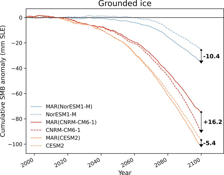
https://doi.org/10.5194/tc-15-1215-2021 The Cryosphere, 15, 1215–1236, 20211228 C. Kittel et al.: Future Antarctic surface mass balance using MAR Figure 9. Reconstructed SMB anomaly (Gt yr−1 ) using CMIP5-RCP8.5 (blue) and CMIP6-ssp585 models (red) over the Antarctic grounded ice (a) and ice shelves (b). Projections are shown using the multi-model mean (solid lines) and the 5 % to 95 % range, corresponding to a standard deviation of ±1.64, across the distribution of individual models (shading). Figure 10. Reconstructed SMB anomaly (Gt yr−1 ) for the CMIP6 models using the ssp126 (blue), ssp245 (green), and ssp585 (red) scenarios over the Antarctic grounded ice (a) and ice shelves (b). Projections are shown using the multi-model mean (solid lines) and the 5 % to 95 % range, corresponding to a deviation of ±1.64, across the distribution of individual models (shading). uncertainties in the downscaling product (Nowicki et al., ample, CNRM-CM6-1 projects a strong near-surface Antarc- 2016), but the significant SMB biases in ESMs in the cur- tic warming (Fig. 1 in this paper and Fig. 1a in Nowicki et al., rent climate (e.g. Krinner et al., 2007; Agosta et al., 2015; 2020), but the related run-off increase is particularly weak Lenaerts et al., 2017b; Palerme et al., 2017; Krinner and (Fig. S13), leading to only very slightly negative anoma- Flanner, 2018) might be a larger source of uncertainties than lies in contrast to MAR(CNRM-CM6-1), which simulates the downscaling itself. Therefore, we compare our MAR widespread negatives anomalies around nearly all the periph- projections forced by NorESM1-M (RCP8.5), CESM2, and eral ice shelves, consistent with a stronger warming (Fig. 7). CNRM-CM6-1 (ssp585) to the ISMIP6-derived SMB used to As highlighted by Fettweis et al. (2020), this suggests that predict the future Antarctic sea level contribution (Seroussi the physics of the models and/or the biases over the cur- et al., 2020) by interpolating the 32 km SMB fields built by rent climate (in particular for the melt) could strongly influ- ISMIP6 on the 35 km MAR grid. ence the projected near-surface changes for identical changes Figure 11 compares future SMB changes (2081–2100 ver- in the free atmosphere. These MAR and ESM differences sus 1995–2014, i.e. the ISMIP6 reference period) projected also highlight the importance of correctly representing the by MAR and the respective forcing ESMs. While the MAR current climate and the need of additional projections rely- projections are relatively insensitive to the forcing ESM for ing on more models, including both RCMs and ESMs. As the same warming (see Sect. 4.2), the comparison between the integrated differences summed over 1995–2100 can be MAR and the forcing ESM reveals large differences inde- larger or as large as the differences between CMIP5-RCP8.5 pendent of the differences due to the higher resolution used and CMIP6-ssp585 or between CMIP6-ssp126 and CMIP6- in MAR that enables high-elevation positive anomalies to be ssp245 (Fig. 12), this also raises the question of the sensitiv- distinguished from low-elevation negative anomalies. For ex- ity to the forcing of ISMIP6 projections, where the SMB is The Cryosphere, 15, 1215–1236, 2021 https://doi.org/10.5194/tc-15-1215-2021
C. Kittel et al.: Future Antarctic surface mass balance using MAR                                                            1229

Figure 11. Comparison between SMB anomalies between 2081–2100 and 1995–2014 (kg m−2 yr−1 ) projected by MAR forced by
NorESM1-M (a), CESM2 (c), CNRM-CM6-1 (e), and the ISMIP6-SMB, directly derived from NorESM1-M (b), CESM2 (d), and CNRM-
CM6-1 (f).

used as an input for performing projections of the total AIS   sub-surface lakes, farther away than the place of its produc-
mass balance (Seroussi et al., 2020).                          tion. The current view suggests that enhanced melt will be
                                                               stored in crevasses or ponds that weaken ice shelves, poten-
5.3   Limitations                                              tially leading to their collapses by hydrofracturing (Scambos
                                                               et al., 2000; Vieli et al., 2007; Pattyn et al., 2018). However,
Our projections suggest a significant ablation by run-off      in some conditions, streams and rivers can transfer surface
as the firn would not absorb all the additional liquid wa-     meltwater laterally and export it into the ocean (Kingslake
ter, whereas almost all surface meltwater refreezes in the     et al., 2017; Pattyn et al., 2018; Dell et al., 2020; Arthur et al.,
snowpack. MAR does not include a liquid-water routing          2020), which might eventually reduce the risk of hydrofrac-
scheme that could either create liquid water flowing over      turing (Bell et al., 2017). Lake formation and meltwater run-
the ice surface or accumulate melted water into surface or     off therefore represent a large uncertainty about the future of

https://doi.org/10.5194/tc-15-1215-2021                                               The Cryosphere, 15, 1215–1236, 2021
You can also read