Development and validation of a numerical wave tank based on the Harmonic Polynomial Cell and Immersed Boundary methods to model nonlinear ...
←
→
Page content transcription
If your browser does not render page correctly, please read the page content below
Development and validation of a numerical wave tank based
on the Harmonic Polynomial Cell and Immersed Boundary
methods to model nonlinear wave-structure interaction
Fabien Robaux1 and Michel Benoit1,2
arXiv:2009.08937v2 [physics.flu-dyn] 26 Aug 2021
1
robaux@irphe.univ-mrs.fr, Aix Marseille Univ, CNRS, Centrale Marseille, Institut de
Recherche sur les Phénomènes Hors-Equilibre (IRPHE), Marseille, France
2
benoit@irphe.univ-mrs.fr, Centrale Marseille, Marseille, France
August 27, 2021
Accepted manuscript for publication, Robaux and Benoit (2021), Journal of Computational Physics,
ISSN 0021-9991.
Abstract
A fully nonlinear potential Numerical Wave Tank (NWT) is developed in two dimensions,
using a combination of the Harmonic Polynomial Cell (HPC) method for solving the Laplace
problem on the wave potential and the Immersed Boundary Method (IBM) for capturing the free
surface motion. This NWT can consider fixed, submerged or wall-sided surface piercing, bodies.
To compute the flow around the body and associated pressure field, a novel multi overlapping
grid method is implemented. Each grid having its own free surface, a two-way communication is
ensured between the problem in the body vicinity and the larger scale wave propagation problem.
Pressure field and nonlinear loads on the structure are computed by solving a boundary value
problem on the time derivative of the potential. The stability and convergence properties of the
solver are studied basing on extensive tests with standing waves of large to extreme wave steepness,
up to H/λ = 0.2 (H is the crest-to-trough wave height and λ the wavelength). Ranges of optimal
time and spatial discretizations are determined and high-order convergence properties are verified,
first without using any filter. For cases with either high level of nonlinearity or long simulation
duration, the use of mild Savitzky-Golay filters is shown to extend the range of applicability of
the model. Then, the NWT is tested against two wave flume experiments, analyzing forces on
bodies in various wave conditions. First, nonlinear components of the vertical force acting on a
small horizontal circular cylinder with low submergence below the mean water level are shown to
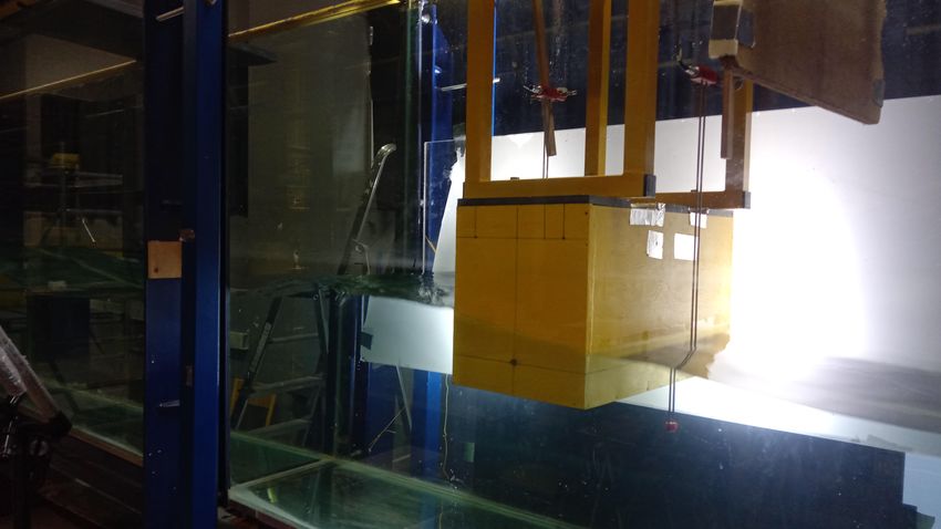
be accurately simulated up to the third order in wave steepness. The second case is a dedicated
experiment with a floating barge of rectangular cross-section. This very challenging case (body
with sharp corners in large waves) allows to examine the behavior of the model in situations at
and beyond the limits of its formal application domain. Though effects associated with viscosity
and flow separation manifest experimentally, the NWT proves able to capture the main features
of the wave-structure interaction and associated loads.
keywords: Fully nonlinear waves, Numerical Wave Tank , Harmonic Polynomial Cell, Boundary
Value Problem, Immersed Boundary Method, Immersed overlapping grids
1
1    Introduction and scope of the study
To model the propagation of oceanic and coastal water waves of high steepness and their interaction
with offshore structures fast and accurate numerical models are needed by scientists and engineers.
Questions related to an accurate estimation of wave loads and structure dynamics in moderate to
severe sea state conditions are of utmost importance for optimizing the design of such structures at
sea and, for instance, assessing their behavior in extreme storm conditions and/or for fatigue analysis
in the life-cycle of the structure. A wide range of models have been developed to predict wave fields
and hydrodynamic loads at any scale, from the simple linear potential boundary element method to
complex Computational Fluid Dynamics (CFD) codes directly solving the Navier-Stokes equations.
    In the last decade, the use of CFD code has become increasingly popular in the scientific com-
munity, see for instance the applications of industrial or research codes like OpenFOAM® (Jacobsen
et al., 2011; Hu et al., 2016; Higuera et al., 2013; Windt et al., 2019), STAR-CCM+ (Oggiano et al.,
2017; Jiao and Huang, 2020), ANSYS-FLUENT (Kim et al., 2016; Feng and Wu, 2019), and REEF3D
(Bihs et al., 2016), just to mention few of them.
    Although these CFD models are well adapted to solve the wave-structure interaction at small scale,
in particular when complex physical processes such as wave breaking, formation of jets, air entrapment
occur, their use is still mostly restricted to a limited number of cases by the computational cost when
targeting applications on ocean domains where the accurate representation of wave propagation is
of first importance. Limitations associated with the employed numerical methods (e.g. numerical
diffusion and difficulty to resolve the dynamics of the free surface) are other reasons which still hinder
the applicability of such models to large scale wave propagation problems. Their performance can be
greatly increased by carefully selecting the different numerical schemes and parameters, to reduce the
computational cost at the expense of some accuracy (Larsen et al., 2019).
    On the other hand, models based on a potential flow approach (i.e. neglecting viscous effects and
assuming irrotational flow) are widely used to describe the dynamics of wave-structure interaction
flows (see e.g. the review by Tanizawa, 2000). Among potential models, simplified linear versions are
often used in the engineering field due to their low computational cost, allowing to capture the main
effects on a wide range of parameters at a contained CPU cost. WAMIT (Lee, 1995), ANSYS-AQWA
(Ansys, 2013) or Nemoh (Fàbregas Flavià et al., 2016) are examples of such linear models. However,
the linear assumption is often used outside its prescribed validity domain, for example in extreme cases
where the allegedly small parameters, usually the wave steepness, becomes large. In those conditions
many aspects of the dynamics of both the incident waves and the wave-body interaction are not
properly modeled.
    Efforts have been done to extend these potential linear models to weakly nonlinear conditions at
second order, mostly by adding terms like the Froude-Krylov forces or the complete Quadratic Transfer
Functions, see e.g. Pinkster (1980) or more recently Philippe et al. (2015). However in some cases,
mostly extreme wave conditions, even third order effects can have a significant effect on the wave load
(see e.g. Fedele et al., 2017). Both the nonlinear wave dynamics and the nonlinear wave-structure
interaction need to be taken into account. In those cases, alternative approaches capturing higher-
order or fully nonlinear effects are needed. Several developments have been made to compute such
nonlinear effect exactly or at high orders in the case of periodic regular waves in uniform water depth.
For example, models based on analytical theories such as the Stokes wave theory (see e.g. Sobey,
1989) or the so-called stream function method (Dean, 1965; Fenton, 1988) can only be applied with
constant or simple geometry of the sea floor. A review of methods to describe wave propagation in a
potential flow framework is given by Fenton (1999).
    High order spectral (HOS) methods are also fast and accurate to compute the flow behavior even
up to large wave steepness. Such methods, though very efficient in computing the wave elevation even
for large domains, might be limited in terms of geometry (complex bodies or variable bathymetry).

                                                    2
They are mostly applied for wave maker modeling (Ducrozet et al., 2012), or to compute the incident
wave field within a more complex method to resolve the wave-structure interactions. For example, in
the SWENSE method (see e.g. Luquet et al., 2007), the diffracted field is computed separately with
a Navier-Stokes based solver.
In order to develop a versatile Numerical Wave Tank (NWT), with the possibility to include
bodies or sea bed with complex geometries, a time domain resolution involving a mesh in the spatial
coordinates appears to be practical at the cost of an increase in the computational load. The commonly
used Boundary Element Method (BEM), in which the Laplace equation is projected onto the spatially
discretized boundaries using the Green’s identities, has been proven to be effective in both 2D and 3D
cases. For example, Grilli and Horrillo (1997) used a high-order BEM method to generate and absorb
waves in 2D. This model was extended to 3D by Grilli et al. (2001). For an overview of work on the
BEM methods up to the end of the 20th century, the reader is referred to Kim et al. (1999). More
recently, Guerber et al. (2012) and Dombre et al. (2019) presented in great detail and implemented
a complete NWT, in 2D and 3D respectively. Note that with the BEM schemes, a special attention
must be given to the treatment of sharp corners (Hague and Swan, 2009).
Another type of time domain wave simulators is volume field solvers. With the cost of increasing
the number of unknowns, the resulting matrix is mostly sparse, allowing the use of efficient solvers.
Both potential and Navier-Stokes solvers can be found in this category. Notable works on NWT based
on the finite difference method (FDM) are given by Tavassoli and Kim (2001), or Engsig-Karup et al.
(2009) (OceanWave3D code). Finite element methods (FEM) were also successfully applied to both
the potential problem (e.g. Ma and Yan, 2006; Yan and Ma, 2007; Engsig-Karup et al., 2016, 2019)
and the Navier-Stokes equations (e.g. Wu et al., 2013).
A different potential model that solves for the volume field was recently proposed by Shao and
Faltinsen (2012, 2014a,b) and tested against several methods including the BEM, FDM and FEM.
This innovative technique, called the "harmonic polynomial cell" (HPC) method, was proven to be
promising both in 2D and 3D (Shao and Faltinsen, 2014a; Hanssen et al., 2015, 2017a). Although
relatively new, this method was used to study a relatively important range of flows and phenomena:
from a closed flexible fish cage (Strand and Faltinsen, 2019) to hydrodynamics lifting problems (Liang
et al., 2015). It was also extended to solve the Poisson equation by Bardazzi et al. (2015). The
numerical aspects of the method were studied in details by Ma et al. (2017) and applied as a 2D NWT
by Zhu et al. (2017).
The treatment of the free surface conditions and body boundary condition can be done in several
ways. A classical and straightforward approach is to use a grid that conforms the boundary shape.
With this method, the boundary node values are explicitly enforced in the linear system. The drawback
of this method is that the grid needs to be deformed at each time step so as to match the free surface.
A lot of solutions have been successfully applied to tackle this issue. For instance, Ma and Yan
(2006) used a Quasi Arbitrary Lagrangian-Eulerian (ALE) method combined with the FEM spatial
discretization to prevent the mesh to have to be regenerated at each time step. Yan and Ma (2007)
extended the mesh conformation technique to include a freely floating body. With this same FEM
discretization, Wu et al. (2013) used in addition an hybrid Cartesian immersed boundary method for
the body boundary condition.
In this work, a NWT based on the HPC method is developed, its convergence assessed, and tested
against both numerical and experimental data. Relaxation zones are used to generate and absorb
waves in a similar manner as in the OpenFOAM® toolbox waveFoam (Jacobsen et al., 2011): the
values and positions of the free surface nodes are imposed from a stream-function theory over a
given distance. The free surface is tracked in a semi-Lagrangian way following Hanssen et al. (2017a)
whereas for the solid bodies, an additional grid fitted to the boundary is defined using the advances
presented in Ma et al. (2017). In order for the body to pierce the free surface, an additional free
3surface marker list is defined in the body fitted grid. "External" and "internal" curves – i.e. free
surface boundaries evolving in the background and body fitted grids respectively – also overlap each
other and communicate through relaxation zones. In order to tackle the singular nodes, a null flow
flux method is imposed on the sharp corners which lay on a Neumann body boundary condition in a
similar manner as in Zhu et al. (2017), but applied at external body corners (described in § 5.4).
The remainder of this article is organized as follows. In § 2 the mathematical formulation of the
potential flow problem is recalled. The numerical methods based on the HPC approach are presented
in § 3, with particular attention devoted to the treatment of the free surface. In § 4, a convergence
study is performed on a freely evolving standing wave case compared to a highly accurate numerical
solution. Numerous tests are performed to determine the optimal ranges of discretization parameters,
first without using any filter. The effects associated with mild filters are then analyzed. The case
of a standing wave of near maximum amplitude is run to confirm the nonlinear capabilities of the
model. Then, a novel fitted mesh overlapping grid method is described and implemented in § 5.
This double mesh strategy is tested on two selected cases in § 6. The first one is an horizontal fixed
circular cylinder, completely immersed although close to the free surface, from Chaplin (1984) and the
second one involves a free surface piercing rectangular barge. That second experiment is an original
campaign done during this study. Results of the present NWT on the two test cases are compared
with experimental data and numerical results from the literature. In § 7, the main findings from this
study and research outlook are summarized and discussed.
2 Fully nonlinear potential flow modeling approach
Three main assumptions are used in the potential model: i. we consider a fluid of constant and
homogeneous density ρ (incompressible flow); ii. the flow is assumed to be irrotational, implying that
∇ × v = 0, where v(x, y, z, t) denotes the velocity field; and iii. viscous effects are neglected (ideal
fluid). Here, (x, y) denote horizontal coordinates, z the vertical coordinate on a vertical axis pointing
upwards, and t the time. The gradient operator is defined as ∇f ≡ (fx , fy , fz )T , where subscripts
denote partial derivatives (e.g. fx = ∂f ∂x ).
The complete description of the velocity field v can thus be reduced to the knowledge of the
potential scalar field φ(x, y, z, t), such that: v = ∇φ. Due to the incompressibility of the flow, the
potential φ satisfies the Laplace equation inside the fluid domain:
∇2 φ = 0, −h(x, y) ≤ z ≤ η(x, y, t) (1)
where η(x, y, t) is the free surface elevation and h(x, y) the water depth relative to the still water
level (SWL). In order to solve this equation, boundary conditions need to be considered. On the time
varying free surface z = η(x, y, t), the Kinematic Free Surface Boundary Condition (KFSBC) and the
Dynamic Free Surface Boundary Condition (DFSBC) apply:
ηt + ∇H η · ∇H φ − φz = 0 on z = η(x, y, t), (2)
1 2
φt + (∇H φ) + gη = 0 on z = η(x, y, t), (3)
2
where ∇H f ≡ (fx , fy )T denotes the horizontal gradient operator and g the acceleration due to gravity.
At the bottom (impermeable and fixed in time), the Bottom Boundary Condition (BBC) reads:
∇H h · ∇H φ + φz = 0 on z = −h(x, y). (4)
4On the body surface, the slip boundary condition expresses that the velocity component of the flow
normal to the body face equals the normal component of the body velocity. Here, we restrict our
attention to fixed bodies, thus, denoting n the unit vector normal to the body boundary, this condition
reduces to:
∂φ
= ∇φ · n = 0 on the body. (5)
∂n
Note that, using the free surface velocity potential and the vertical component of the velocity at
the free surface, defined respectively as:
φ̃(x, y, t) = φ(x, y, η(x, y, t), t) (6)
∂φ
w̃(x, y, t) = (x, y, η(x, y, t), t) (7)
∂z
the KFSBC and the DFSBC can be reformulated following Zakharov (1968) as:
ηt = −∇H η · ∇H φ̃ + w̃(1 + (∇H η)2 ) (8)
1 1
φ̃t = −gη − (∇H φ̃)2 + w̃2 (1 + (∇H η)2 ) (9)
2 2
It can be noted that the Laplace eq. (1), the BBC (eq. (4)) and the body BC (eq. (5)) are all linear
equations. Thus, the nonlinearity of the problem originates uniquely from the free surface boundary
conditions (eqs. (2) and (3)) or (eqs. (8) and (9)). A classical approach at that point is to assume that
surface waves are of small amplitude relative to their wavelength, so that these boundary conditions
can be linearized and applied at the SWL (i.e. at z = 0). Here, we intend to retain full nonlinearity
of wave motion by considering the complete conditions (eqs. (8) and (9)). These two equations are
used to compute the time evolution of the free surface elevation η and the free surface potential φ̃.
This requires obtaining w̃ from (η, φ̃), a problem usually referred to as Dirichlet-to-Neumann (DtN)
problem.
For given values of (η, φ̃), the DtN problem is here solved by solving a BVP problem in the
fluid domain on the wave potential φ(x, y, z, t), composed of the Laplace equation (eq. (1)), the
BBC (eq. (4)), the body BC (eq. (5)), the imposed value φ(z = η) = φ̃ (Dirichlet condition) on the
free surface z = η, supplemented with boundary conditions on lateral boundaries of the domain (of
e.g. Dirichlet, Neumann, etc. type). The numerical methods to solve the BVP are presented in the
next section.
3 The Harmonic Polynomial Cell method (HPC) with immersed
free surface
3.1 General principle of the HPC method
In order to solve the above mentioned BVP at a given time, the HPC method introduced by Shao
and Faltinsen (2012) is used. It is briefly described here, and more details can be found in Shao and
Faltinsen (2014b), Hanssen et al. (2015, 2017a), Hanssen (2019) and Ma et al. (2017). In this work,
the HPC approach is implemented and tested in 2 spatial dimensions, i.e. in the vertical plane (x, z),
for a wide range of parameters.
5The fluid domain is discretized with overlapping macro-cells which are composed of 9 nodes in
2 dimensions. Those macro-cells are obtained by assembling four adjacent quadrilateral cells on an
underlying quadrangular mesh. The four cells of a macro-cell share a same vertex node, called the
"central node" or "center" of the macro-cell. A typical macro-cell is schematically shown in fig. 1, with
the corresponding local index numbers of the 9 nodes. With this convention, any node with global
index n has the local index "9" in the considered macro-cell and is considered as an interior fluid
point, whereas for example node with local index "4" can either be a fluid point or a point lying an a
boundary. In the case node “4” is also an interior fluid point, it defines a new macro-cell overlapping
the original one: nodes denoted 6,7,8,9,2 and 1 in fig. 1 also belong to this macro-cell centered by “4”.
6 7
8
4 5
9
3
1 2
Figure 1: Definition sketch of 9-node macro-cell used for the HPC method, with local numbering of
the nodes
In each macro-cell, the velocity potential is approximated as a weighted sum of the 8 first harmonic
polynomials (HP), the latter being fundamental polynomial solutions of the Laplace eq. (1). A dis-
cussion about which of the HP are to be chosen is given in Ma et al. (2017). Here, we follow Shao and
Faltinsen (2012), and select all polynomials of order 0 to 3 plus one fourth-order polynomial, namely:
f1 (x) = 1, f2 (x) = x, f3 (x) = z, f4 (x) = xz, f5 (x) = x2 − z 2 , f6 (x) = x3 − 3xz 2 , f7 (x) = −z 3 + 3x2 z
and f8 (x) = x4 − 6x2 z 2 + z 4 . Here, x = (x, z) represents the spatial coordinates. Thereafter, we
define x̄ = x − x9 the same spatial coordinate in the local reference frame of the macro-cell, with x9
being the center node of the macro cell. From a given macro-cell, the potential can be approximated
at a location x as:
8
X
φ(x) = bj fj (x̄) (10)
j=1
As every HP is a solution of the Laplace eq. (1) which is linear, any linear combination of them is
also solution of this equation. Thus, the goal now becomes to match the local expressions (LE) given
by eq. (10): if this equation is satisfied at each node (j = 1, ..., 8) of each macro-cell, a solution of the
BVP is available everywhere. For that reason, macro-cells overlap each other. Note that this study
deals with 2D problems, but the method can be extended to 3D cases as shown by Shao and Faltinsen
(2014a) considering cubic-like macro-cells with 27 nodes.
The first objective is to determine the vector of coefficients bj , j = 1, ..., 8 for the selected macro-
cell. Recalling that eq. (10) should be verified at the location of each point of the macro-cell (with
local index running from 1 to 9), this equation applied at the 8 neighboring nodes (1 − 8) of the center
yields:
68
X
φi = φ(xi ) = bj fj (x̄i ) for i = 1, ..., 8 (11)
j=1
which represents, in vector notation, a relation between the vector of size 8 of the values of the potential
φi at the outer nodes with the vector of size 8 of the bj coefficients. The 8x8 local matrix linking
these two vectors is denoted C, and defined by Cij = fj (xi ). Note that C is defined geometrically,
thus it only depends on the position of the outer nodes i relatively to the position of the central
node. C can be inverted and its inverse is denoted C−1 . The bj coefficients are then obtained for the
given macro-cell as a function of the potentials at the 8 neighboring nodes of the central node of that
macro-cell:
8
X
−1
bj = Cji φi for j = 1, ..., 8. (12)
i=1
Injecting this result into the interpolation eq. (10), a relation is found providing an approximation for
the potential at any point located inside the macro-cell using the values of the potential of the eight
surrounding nodes of the central node:
X 8 X8
−1
φ(x) = Cji fj (x̄) φi (13)
i=1 j=1
This equation will be referred to as local expression (LE) of the potential. It will be used to
derive the boundary conditions equations and the fluid node equations that need to be solved in the
BVP. Also note that this LE provides a really good interpolation function that can be used for every
additional computation once the nodal values of the potential are known (i.e. potential derivatives at
the free surface or close to the body to compute the pressure field).
Note that the accuracy of LE depends only on the geometry: coordinates at which this equation
is applied, shape of the macro-cell, etc. Those dependencies are investigated in details by Ma et al.
(2017).
3.2 Treatment of nodes inside the fluid domain
We first consider the general case of macro-cells whose central node is an interior node of the fluid
domain. Applying the LE (eq. (13)) at the central node yields a linear relation between the values of
the potential at the nine nodes of this macro-cell:
X 8 8
X
−1
φ9 = φ(x9 ) = Cji fj (x̄9 ) φi (14)
i=1 j=1
We may further simplify this equation by noting that, as x̄9 = (0, 0) in local coordinates, all fj (x̄9 )
vanish, except f1 (x̄9 ) which is constant and equal to 1. Equation (14) then simplifies to:
8
X
−1
φ9 = C1i φi (15)
i=1
meaning that only the first row of the matrix C−1 is needed here.
7In order to solve the global potential problem, i.e. to find the nodal values of the potential at all
grid points (whose total number is denoted N ), a global linear system of equations is formed, with
general form A.φ = B, or:
N
X
Akl φl = Bk for k = 1, ..., N. (16)
l=1
where k and l are global indexes of the nodes. For each interior node in the fluid domain, with global
index k and associated macro-cell, an equation of the form of eq. (15) allows to fill a row of the
global matrix A. This row k of the matrix involves only the considered node and its 8 neighboring
nodes, making the matrix A very sparse (at most 9 non-zero elements out of N terms). Moreover,
the corresponding right-hand-side (RHS) term Bk is null. Note that all the 8 neighboring nodes of
the macro-cell associated with center k should also have a dedicated equation in the global matrix in
order to close the system.
3.3 Nodes where a Dirichlet or Neumann boundary condition is imposed
If a Dirichlet boundary condition with value φD of the potential has to be imposed at the node of
global index k, the corresponding equation is simply φk = φD , so that only the diagonal element of
the global matrix is non-null and equal to 1 for the corresponding row k: Akl = δkl ∀l ∈ [1, N ]. The
corresponding term on the RHS is set to Bk = φD .
If a Neumann condition has to imposed at a given node of global index k, the relation set in the
global matrix is found through the spatial derivation along the imposed normal n of the LE (eq. (13))
of any macro-cell on which k appears. In practice, the macro-cell whose center is the closest to the
node k is chosen, and we then use:
X8 X8
−1
∇φ(xk ) · n = Cji ∇fj (x̄k ) · n φi (17)
i=1 j=1
Thus, a relation is set in the row k of the global matrix to enforce the value of Bk = ∇φ(xk ) · n
at position xk . In that case, a maximum of 8 non-zero values appear in this row on the global matrix
as the potential of the central node of the macro-cell does not intervene here.
3.4 Treatment of the free surface
As already mentioned, in order to solve the BVP at a given time-step, the system of equations needs
to be closed, meaning that each neighbor of a node in the fluid domain should have a dedicated
equation. We consider now the case of nodes lying on or in the vicinity of the (time varying) free
surface. The free surface potential should be involved here, either directly at a node fitted to the free
surface through a Dirichlet condition described in the previous sub-section, or through alternative
techniques.
For instance, an Immersed Boundary Method (IBM) was first suggested in the HPC framework by
Hanssen et al. (2015) to tackle body boundary conditions. More recently, Ma et al. (2017) compared a
modified version of the IBM with two different multi-grid (MG) approaches (fitted or combined with
an IBM) for both body and free surface boundary conditions. Hanssen et al. (2017a) and Hanssen
et al. (2017b) also made in-depth comparisons of the MG and IB approaches, focusing on the free
surface tracking. Both methods showed promising results. Zhu et al. (2017) introduced a similar yet
slightly different IB approach with one or two ghost node layers, then realized a comparison between
8this IB approach and the original fitted mesh approach. In the present work, the IBM was chosen for
the treatment of the free surface, though the fitting mesh method is shortly described thereafter.
3.4.1 Fitted mesh approach for the free surface
The first possibility is to fit the mesh to the actual free surface position at any time when the BVP
has to solved. The mesh is deformed so that the upper node at any abscissa always lies on the free
surface. That way, the computational domain is completely closed and the free surface potential
is simply enforced as a Dirichlet boundary condition at the correct position z = η as explained in
§ 3.3. With this approach, the algorithm, given the boundary values at the considered time, can be
summarized as:
• Deform the mesh to fit the current free surface elevation,
• Build and then invert the local geometric matrices C,
• Fill the global matrix A and RHS B, using the corresponding Dirichlet conditions at nodes lying
on the free surface,
• Invert the global problem to obtain the potential everywhere
Recently, Ma et al. (2017) pointed out that the HPC method efficiency (in terms of accuracy and
convergence rate) is greatly improved when a fixed mesh of perfectly-squared cells is used. In this work,
the negative effects of a deforming mesh outlined in the previous subsection were also encountered.
Especially, for some particular cell shapes, a high increase of the local condition number was observed,
leading to difficulty of matrix inversion and important errors on the approximated potential. As a
consequence, results were highly dependent on the mesh deformation method employed, especially in
the vicinity of a fixed fully-immersed body.
3.4.2 Immersed free surface approach
In order to work with regular fixed grids, an IBM technique was developed and implemented to
describe the free surface dynamics. Hanssen et al. (2015) introduced a first version of this method
applied on the boundaries of a moving body. This method was recently extended to the free surface
and compared to a fitted MG method by Ma et al. (2017) and Hanssen et al. (2017a). In the current
work, a semi-Lagrangian IB method introduced by Hanssen et al. (2017a) is chosen.
In this method, the free surface is discretized with markers, evenly spaced and positioned at each
vertical intersection with the background fixed grid, as shown in fig. 2. Those markers are semi-
Lagrangian in such a way that they are only allowed to move vertically, following eqs. (8) and (9).
At a given time, every node located below the free surface (i.e. below a marker) is considered as
a node in the fluid domain ("fluid" node), and defines a macro-cell with its 8 neighbors. The global
matrix is classically filled with the local expression (eq. (13)) at those nodes. As a consequence,
in order to close the system, each neighbor of a node just above the free surface must also have a
dedicated equation in the global matrix. These neighbors, represented with grey circles on fig. 2, are
denoted as "ghost" nodes. The chosen equation to close the system at a node of this type is the local
expression (eq. (13)) applied at the marker position in a given macro-cell:
X8 X8
−1
φm = Cji fj (x̄m ) φi (18)
i=1 j=1
9Ghost nodes
Centers of macro-cell used for ghost nodes
Markers on the free surface
Inactive nodes
Figure 2: Schematic representation of the immersed free surface in a fixed grid
where x̄m = (xm , η(xm )) − xc is the position of the marker in the macro-cell’s reference frame (xc
is the global position of the center node of the chosen macro-cell) and φm its potential (known at
this stage). This ensures that the potential at the free surface point is equal to the potential at the
position of the marker from the interpolation equation. In other words, if one wants to interpolate
the computed field φ at the particular location of the marker xm , the results should be consistent and
yield the potential φm .
−1
Note that this eq. (18) is cell dependent (through Cji , the involved φi and the position of the
center node xc ), but also depends on the chosen marker (through xm and φm ). The only mathematical
restriction on the choice the macro-cell to consider is that the ghost point potential should intervene
as one of the φi in order to impose the needed constraint at this point.
An important note is that the latter eq. (18) is not dependent on the ghost point in any fashion.
This implies that if the same couple (marker, macro-cell) is chosen to close the system at two different
ghost points, the global matrix will have two strictly identical rows. Its inversion would thus not be
possible. Particularly, two vertically aligned ghost points cannot use the same macro-cell equation
at the same marker position. Here stands the difference between the IB method of Hanssen et al.
(2017b), Ma et al. (2017) and the one chosen by Zhu et al. (2017). Zhu et al. (2017) decided to only
impose the marker potential once in the first layer (or two first layers) and to constraint the upper
potentials to an arbitrary value (in practice if the point is not used directly, the potential is set to
the first point below which potential is used). The method used during this work is closer to the one
by Hanssen et al. (2017b) and Ma et al. (2017): if a node needs a constraint but does not have a
marker directly underneath (case of two ghost points vertically aligned), the ghost point on the top
should invoke the local expression of the macro-cell centered on the closest fluid point instead of the
cell centered on the vertically aligned fluid point (case indicated by an arrow in fig. 2). With that
method, in such a situation, the potential of the selected marker – i.e. vertically aligned with the two
ghost points – is imposed twice in two different adjacent macro-cells. A comparison between those
two methods had not been conducted and would be of great interest.
Regardless of the kind of IB method used, the main goal is achieved: it is not needed to deform
the mesh in time. As a consequence, the computation and inversion of the local (geometric) matrices
is only done once, at the beginning of the computation. However, a step of identification of the type
of each node, which was proven to be time consuming, is needed instead. Note that this identification
algorithm could be greatly improved and is relatively slow in its current implementation. The general
algorithm at one time step becomes:
10• Identify nodes inside the fluid domain,
• Identify ghost nodes needed to close the system, associated markers and macro-cells,
• Fill global matrix A and RHS B,
• Invert global problem to obtain the potential everywhere,
3.5 Linear solver and advance in time
To solve the global linear sparse system of equations, an iterative GMRES solver, based on Arnoldi
inversion, was used for all computations. The base solver was developed by Saad (2003) for sparse
matrix (SPARSEKIT library), and includes an incomplete LU factorization preconditionner. In the
current implementation, a modified version of the latter is used with the improvement proposed by
Baker et al. (2009). Except for stalling during the study of a standing wave at very long time, this
solver was proven to be robust. Improvements of the construction step of the global matrix could
further be made in order to increase the efficiency of its inversion. Also, the initial guess in the
GMRES solver could also be improved taking advantages of the already computed potential values.
The number of inner iterations of the GMRES algorithm was chosen as m ∈ [30, 60] and the iterative
solution is considered converged when the residual is lower that 5.10−9 .
Marching in time thanks to eqs. (8) and (9) yields the free surface elevation and the free surface
potential at the next time step. Note that the steps of computing the RHS terms of these equations
are straightforward for most terms directly from the local expression (eq. (13)) of the closest macro-
cell. In addition, the spatial derivative of η is computed with a finite difference method. A centered
scheme of order 4 is chosen for this work with the objective to maintain the theoretical order 4 of
spatial convergence provided by the HPC method.
In order to integrate eqs. (8) and (9), the classical four-step explicit Runge-Kutta method of order
4 (RK4) was selected as time-marching algorithm. During a given simulation, the time step (δt) was
chosen to remain constant. Its value is made nondimensional by considering the Courant-Friedrichs-
Lewy (CFL) number Co based on the phase velocity C = λ/T , where λ is the wavelength and T the
wave period:
Cδt λ/δx
Co = = (19)
δx T /δt
The CFL number thus corresponds to the ratio of the number of spatial grid-steps per wavelength
(Nx = λ/δx) divided by the number of time-steps per wave period (Nt = T /δt), i.e. Co = Nx /Nt .
3.6 Computation of the time derivative of the potential
The pressure inside the fluid domain is obtained from the Bernoulli equation:
∂φ 1
p(x, z, t) = −ρ + 2
(∇φ) + gz (20)
∂t 2
This equation is used in every potential based NWT in order to obtain the wave loads. For this reason,
the knowledge of the time derivative of the potential is required. In a first attempt, the time derivative
of the potential was estimated using a backward finite difference scheme. However, this method is not
well suited when important variations of the potential are at play. Moreover, in the case of the IB
method, it is not possible to obtain the value of the pressure at a point that was previously above the
free surface, and thus for which a time derivative of the potential cannot be computed by the finite
difference scheme.
11A fairly accurate method is to introduce the (Eulerian) time derivative of the potential as a new
∂φ
variable φt = and to solve a similar BVP as described previously on this newly defined variable,
∂t
noting that φt has to satisfy the same Laplace equation as φ in the fluid domain. This method, first
used by Cointe et al. (1991); Tanizawa (1996), has been recently applied by e.g. Guerber (2011) in
the BEM framework or by Ma et al. (2017) in the HPC method.
Note that the local macro-cell matrices and coefficients, which are only geometrically dependent,
do not change. In the different expressions presented above that are used to fill the global matrix,
the coefficients linking the different potentials are not time dependent. Thus, the matrix to invert is
exactly the same for the φt field and the φ field. However, the boundary conditions on φ and φt might
differ, leading to different RHS. This is the case only when the RHS on φ is different from zero, as for
example, for free surface related closure points.
Remember that the equations at a (non-moving) Neumann condition and at a point inside the fluid
domain yield a zero value in the RHS, and thus the equations at those points are exactly the same
for the potential variable and for its derivative. At a (non-moving) Dirichlet boundary condition, one
would simply impose φt = 0 instead of φ = φD . At the IB ghost points (i.e. to enforce the free surface
condition), the φt is imposed to match the derivative of the potential with respect to time, known at
the marker positions from eq. (9). Even though the global matrices are exactly the same, the RHS
being different and the chosen resolution method being iterative (GMRES solver), the easiest way
is just to solve twice the almost same problem. A more clever way could maybe be investigated by
taking advantage of the previous inversion, but this is left for future work.
4 Validation and convergence study on a nonlinear standing
wave
4.1 Presentation of the test-case
The first case consists in simulating a nonlinear standing wave in a domain of uniform water depth
h whose extent is equal to one wavelength λ. This case is quite demanding as the wave height H
(difference between the maximum and minimum values of free surface elevation at antinode locations)
is fixed by choosing a large wave steepness H/λ = 10% (or kH/2 = π/10 ≈ 0.314). We also choose to
work in deep water conditions by selecting h = λ = 64 m (or kh = 2π ≈ 6.28). The water domain at
rest is thus of square shape in the (x, z) plane, as illustrated in fig. 3.
Initial elevations of free surface η(x, t = 0) are computed from the numerical method proposed by
Tsai and Jeng (1994). The initial phase is chosen such that the imposed potential field is null at t = 0
at any point in the water domain. This initial state corresponds to a maximum wave elevation at the
beginning and the end of the domain (x/λ = 0 and 1), and a minimum wave elevation at the center
point of the domain (x/λ = 0.5), these three locations being antinodes of the standing wave.
Wall boundary conditions are enforced as null Neumann conditions, i.e. ∇φ · n = 0 on the three
wet walls, where n is the considered wall normal vector.
The wave is freely evolving under the effect of gravity: in theory one should observe a fully periodic
motion without any damping as the viscosity is neglected. At each time step, a spatial L2 (η) error
on η is computed relative to the theoretical solution of Tsai and Jeng (1994) (denoted η th hereafter),
and normalized with the wave height:
v
u np
1u 1 X 2
L2 (η, t) = t (η(xi , t) − η th (xi , t)) (21)
H np i=1
12H = 6.4m
h = 64m
L = 64m
Figure 3: Schematic representation of the nonlinear standing wave with steepness H/λ = 10% at
t = 0. Mesh grid represented with Nx = 20.
where i represents the index of a point on the free surface and np the total number of points on the
free surface.
4.2 Evolution of L2 (η) error with space and time discretizations
The result of this L2 (η)-error is represented as a color map at four different times t/T = 1, 10, 50
and 100 in fig. 4 as a function of the number of nodes per wavelength (Nx = λ/δx, where δx is the
spatial step-size) and the CFL number Co (defined in § 3.5). Wide ranges of the two discretization
parameters are explored, namely Nx ∈ [10, 90] and Co ∈ [0.05, 4.0]. Simulations that ran till the end of
the requested duration of 100T are represented with coloured squares. A circle is chosen as a marker
when the computation breaks down before the end of that duration. Nonetheless the markers are
colored if the computation did not yet diverge at the time instant shown on the corresponding panel.
Results of fig. 4 show that a large number of simulations were completed over this rather long
physical time of 100T . In this §, no filter were used, so some of the numerical simulations tend to
be unstable for extreme values of the discretization parameters. For instance, when Co ≤ 1, the
computation is mostly unstable and breaks down: before 50T when Nx is small (i.e. below 40) and
between 50T and 100T when Nx is larger. Note that Co = 1 corresponds to a time step ranging from
Nt = T /δt = 10 to 90, for Nx = 10 and 90 respectively. This value of Co = 1, and associated time
step, is the lower stable limit exhibited by these simulations.
On the other hand, when the Co is too high (i.e. larger than 3.5) instabilities also occur almost
at the beginning of the simulation (t/T < 10), particularly when Nx is small. For very small Nx (in
the range 10-15) and whatever the Co , the computation tends to be unstable. This is probably due to
the discretization of the immersed free surface being the same as the discretization of the background
mesh. A coarse discretization of the free surface leads to an inaccurate computation of the spatial
derivative of η: instabilities may then occur.
A suitable range of parameters is thus determined to avoid instabilities: 1.5 ≤ Co ≤ 3.5 and
40 ≤ Nx ≤ 90. This zone is represented in fig. 4 as a rectangular box with a dashed contour. In that
zone, all the computations ran with the requested time step over a duration of 100T . Note that the
CPU cost scales with Nx2 Nt ∼ Nx3 /Co and thus the most expensive computations in this stable zone
135.6 10 1
4 t/T=1 4 t/T=10
3 3 10 1
CFL
2 2
1 1 10 2
0 0
L2 ( )
20 40 60 80 20 40 60 80 10 3
4 t/T=50 4 t/T=100
3 3
10 4
CFL
2 2
1 1 10 5
0 0
2.2 10 6
20 40 60 80 20 40 60 80
Nx Nx
Figure 4: L2 error on η on the nonlinear standing wave case at four time instants (t/T = 1, 10, 50
and 100) as a function of the spatial and temporal discretizations. The color scale indicates the L2 (η)
error respective to the theoretical solution by Tsai and Jeng (1994). See text for explanations on the
significance of the markers shapes.
are approximately 25 times slower than the least expensive ones in the same zone. Also note that the
lowest error is almost systematically reached in this zone. The L2 (η) error is as small as 2.10−6 after
1T . After 100T , the lowest error is approximately 10−4 . Moreover, the evolution of the value of the
error is qualitatively consistent with the mesh refinement and time refinement.
The stability was not assessed for finer mesh than Nx = 90 points per wave length, due to
increasing computation cost on one hand, and the fact that finer resolutions would lie out of the
range of discretizations targeted for real-case applications. In addition, at long time, a discretization
of Nx = 90 already exhibits behavior that does not match the expected convergence rate, as will be
discussed hereafter in greater detail.
4.3 Convergence with time discretization
In order to study the convergence of the method in a more quantitative manner, the L2 (η) error is
shown as a function of the Co number for different spatial discretizations Nx at t/T = 1 in fig. 5a and
at t/T = 100 in fig. 5b. A Coα regression line is computed and fitted on the linear convergence range
of the log-log plot of the error. That will be called "linear range" for simplicity, though it corresponds
to an algebraic rate of convergence of the error. Note that this linear range corresponds exactly to the
zone in which the computations remain stable (with the exception of one particular point at t/T = 100
and Nx = 90 excluded from the determination of the convergence rate). At t/T = 1, the minimum
error is, as expected, obtained for small Co numbers and large Nx : L2 (η) ∼ 10−5 in the linear range
and the minimal error reached is 2.10−6 for the finer discretization Nx = 90. The algebraic order of
convergence is close to 4. This was expected as the temporal scheme is the RK4 method at order 4.
Moreover, at this early stage of the simulation the error decreases with a power 4 law only when Co
14& 1.0. The lowest errors are achieved at Co ≈ 0.75. Below that Co number, a threshold is met: the
error remains constant when the time step (and Co number) is further decreased; it is then controlled
by the spatial discretization. It is also possible to note that the CFL number Co seems to be a relevant
metric when testing the convergence of the method: the range of Co in which the results converge is
the same across the 4 considered spatial discretizations.
10−2
Nx30 :x3.75 Nx30 :x4.99
Nx50 :x3.66 Nx50 :x6.03
−1
Nx70 :x3.68 10 Nx70 :x5.32
10−3 Nx90 :x3.70 Nx90 :x5.07
L2 (η)
L2 (η)
10−2
10−4
10−3
−5
10
t/T=1 t/T=100
10−4
0.05 0.1 0.20 0.50 1.0 1.502.0 3.0 0.05 0.1 0.20 0.50 1.0 1.502.0 3.0
CFL CFL
(a) t/T = 1 (b) t/T = 100
Figure 5: Convergence of the L2 error on η (crosses) with respect to the temporal discretization at two
different physical times: t/T = 1 (left panel) and t/T = 100 (right panel). The spatial discretization
is fixed for a given line. Solid lines represent power regression of the error in the "linear range", the
computed power is reported in the legend of the fitted straight lines.
Remark 1 Significant differences in terms of Co with the work of Hanssen et al. (2017a) have to
be stressed. In their simulations the chosen numbers of points per wavelength were similar to the
ones used here (Nx ∈ [15, 90]), but the time step was constant and fixed at a small value of δt/T =
1/Nt = 1/250. This value yields a Co between 0.06 and 0.36. This range of Co was shown to be
out of the domain of convergence in time in our case. For the same Co (and apparently the same
RK4 time scheme), the computation is indeed converged with respect to the time discretization and
yields low error during the first periods, but instabilities then occur when the wave are freely evolving
on a longer time scale. Hanssen et al. (2017a) also encountered instabilities with this IB method.
To counteract these instabilities, they used a 12th order Savitzky-Golay filter in order to suppress, or
at least, attenuate them. No filtering nor smoothing was used in our simulations. This may explain
the differences of behavior with Hanssen et al. (2017a) in terms of Co number. Similarly, in Zhu
et al. (2017), also with the RK4 time scheme, the time-step is chosen as δt/T = 1/200 for a spatial
discretization of δx = h/10. Converted to our numerical case, this would correspond to Nx = 100,
and so a Co fixed at 0.5. During the investigations of Ma et al. (2017) on periodic wave propagation,
their spatial discretizations ranged from Nx = 16 to Nx = 128. The equivalent Co number is thus
comprised between 0.4 and 3.2.
At long time t/T = 100 (see fig. 5b), the error behaves differently. First, the error is approxi-
mately one order of magnitude higher compared to the time t/T = 1, but the convergence rate is also
slightly different, actually higher. As a matter of fact, at t/T = 100, an order 4 of convergence is still
found on the wave period and on the amplitude of the computed wave: fig. 6 shows the dependence
in CFL of the error in wave period and amplitude at the center of the domain x/λ = 0.5 at t/T = 100
for a fixed Nx = 30 as a function of the CFL number Co . The reference case used here is the one with
15Nx = 100 at Co = 0.05 computed on one period. On a given case, the period is computed through the
mean time separating two successive maximums, then a sliding Fast Fourier Transformation (FFT) is
performed to obtained an accurate estimation of the amplitude of the free surface elevation.
err(A) x/λ = 0.5 :x3.97
err(T) x/λ = 0.5 :x4.10
L2 (η) :x5.25
10−1
relative error
10−2
10−3
t/T=100
1.5 2 2.5 3 3.5
CFL
Figure 6: Convergence of the error on wave period and amplitude of the wave elevation at x/λ = 0.5
for Nx = 30. The L2 (η) error -combination of both- is also added.
However, the behavior of the L2 (η) error results from a combined effect of both the error on the
wave period and the error on the amplitude. The relative effect of those errors on the total error
is analyzed in detail in appendix A, and a brief summary is given here. Let e be the relative error
between two cosine functions. The first is the target function and the second one tends to the first
one in amplitude as a = fA d4 and in period as t = fT d4 . Here d is a discretization variable -either
Co or 1/Nx in our case-, which drives the convergence. fA and fT are constants with respect to d. At
a whole number of periods – i.e. t/T ∈ N – a Taylor expansion of e when d → 0 can be performed:
t2 2 8 t t2
e = fA d4 + 2π 2 2
fT d + (2π fT3 − 2fA π 2 2 fT2 )d12 + O(d16 ) (22)
T T T
Note that fA depends on t/T because the error on amplitude increases with time (in practice a linear
dependence was observed at long time, i.e. fA = f¯A t/T ). However fA and fT should not depend
on the convergence parameter d. The order 8 of convergence should disappear for small enough d
whatever t/T . In that case, the error on period is negligible compared to the error on amplitude:
this results from the presence of the cosine, which elevates the error to the power 2. However, if the
error in amplitude fA increases in time slower than t2 fT2 , there exists a time after which the error
on the wave period will play an important role (order 8 will be predominant). This effect is thought
to explain the seemingly high order of convergence of the L2 (η) error in fig. 5b. Appendix A shows
detailed comparisons at t/T = 100 with values of fA and fT extracted from our results.
4.4 Convergence with spatial discretization
The convergence with spatial refinement (i.e. as a function of Nx = λ/δx) is analyzed in the same
way and shown in fig. 7. The order of convergence in space is again 4. Due to the choice of the set
of HP including polynomials up to order 4, and the fact that the finite difference scheme of order 4
is used to compute the derivatives of free surface variables, this order 4 was the expected order of
convergence.
1610−1
t/T=1 t/T=100
10−2 10−1
L2(η)
L2(η)
10−3 10−2
CFL1.5 :x−3.69 CFL1.5 :x−5.36
10−4 10−3
CFL2.0 :x−3.82 CFL2.0 :x−5.57
CFL2.5 :x−3.86 CFL2.5 :x−5.96
CFL3.0 :x−4.01 CFL3.0 :x−5.76
10−5 CFL3.5 :x−3.90 CFL3.5 :x−6.17
10−4
20 30 40 50 60 70 80 90 20 30 40 50 60 70 80 90
Nx = λ/dx Nx = λ/dx
Figure 7: Convergence of the L2 error on η in mesh refinement, with temporal discretization fixed.
Solid lines correspond to the power regression of the error.
At long time the convergence rate exhibits the same behavior as shown in the convergence with
time resolution. The latter comments concerning the long time evolution of the error still holds (with,
here, d ≡ δx), and is again thought to explain the increasing order of convergence of the total error
L2 (η) with time. Of course the values of the corresponding constants fA and fT are different. Another
effect also occurs: when the Co number increases, so does the order of convergence. This small yet
clear effect at time t/T = 100 is not completely understood. It would mean that the value of fT
increases faster with the Co number than the value of fA does.
4.5 Effect of filtering the free surface variables
Nx30 noFilter Nx50 noFilter Nx90 noFilter
Nx30 SG(13,8) Nx50 SG(13,8) Nx90 SG(13,8)
Nx30 SG(13,6) Nx50 SG(13,6) Nx90 SG(13,6)
10−1
10−2 10−1
10−3
10−2
L2 (η)
L2 (η)
10−4
10−3
10−5
t/T=1.0 t/T=100.0
10−4
0.05 0.1 0.20 0.50 1.0 1.502.0 3.0 0.05 0.1 0.20 0.50 1.0 1.502.0 3.0
CFL CFL
Figure 8: Convergence of the L2 error on η with respect to the CFL number at two different physical
times: t/T = 1 (left panel) and t/T = 100 (right panel), showing the effect of Savitzky-Golay
filters SG(13,6) (triangles) and SG(13,8) (circles) in comparison to simulations run without any filter
(crosses).
As shown in the previous sub-section, stable computations are obtained for a range of spatial and
17temporal discretizations without any filtering. The phenomenon limiting this range is the so-called
"sawtooth instability" developping on the free surface immersed boundary. In this sub-section, we
evaluate the effect of applying a centered Savitzky-Golay filter (Savitzky and Golay, 1964) on the
achievable range of discretization parameters. This filter is denoted SG(N ,O) where N is the total
number of points of the filter (i.e. (N − 1)/2 points are involved on each side of a considered node)
and O its order. An in-depth investigation on the effect of such filter is given in Ducrozet et al. (2014).
The filter is applied to the free surface elevation first. Afterwards, a correction step of the free
surface potential was shown to be necessary to avoid the growth of instabilities: the free surface
potential is enforced from an interpolation using the LE eq. (13) at the updated point elevation. The
same filter is then applied to the newly obtained free surface velocity potential. This procedure is
applied once per time step, after the resolution of the main BVP.
Figure 8 shows the dependence on CFL of the free surface elevation error after 1 and 100 wave
periods without filter (similar curves as in fig. 5) and with two SG filters with N = 13 and orders
O = 6 and 8 respectively. A great improvement on the width of the accessible parameter range is
obtained, especially for the long simulation period (t/T = 100), for which almost all the simulations
ran to their target duration.
It can be noted that no significant gain in terms of accuracy can be obtained at short time
(t/T = 1). Rather, the coarsest mesh resolutions exhibit a significant increase in total error. When
increasing the spatial grid step δx at fixed CFL value, two opposite effects are present: 1) the time
step δt increases, leading to a reduced number of filter applications for a given simulation duration,
2) however, each application of the SG filter increases in strength as shown by Ducrozet et al. (2014).
Thus, as the total error increases as the mesh gets coarser, it is deduced that the second effect is
dominant over the first one. This effect is more marked with SG(13,6) in comparison with SG(13,8).
It is also possible to observe the former effect at fixed Nx with decreasing CFL, as the total error
increases.
After a longer time evolution, benefits of the filter can be pointed out: lower CFL can be used
without breaking the simulation. For some spatial discretizations, this leads to a lower minimal
achievable error. For example, at Nx = 50 the simulation at CFL = 0.75 is stabilized, leading to the
best achieved accuracy, slightly better than with Nx = 90, CFL = 2.
Overall, this type of filter, in particular used with SG(13,8) setting, appears to be able to contain
the growth of instabilities and allows to run simulations with large intervals of discretization param-
eters. Though an increase in error is noted in some cases characterized by low CFL values at short
times, the long term results are improved regarding both the number of stable simulations and the
final error levels.
Because good enough stability was denoted in a relatively large range of Nx , CF L when the
simulated time is contained (≤ 100T ), the use of a filter was not found to be necessary for the rest of
the computations presented in this paper, unless stated otherwise.
4.6 Highly nonlinear standing wave
Though the standing wave case considered above has a rather high steepness (H/λ = 10%), in order
to approach the maximal achievable standing wave height, a test case inspired from Ducrozet et al.
(2014) was simulated. A nonlinear regular wave train with incident wave steepness HI /λI = 7.5%
is generated at the left boundary of the domain using a stream-function solution of order 20. These
waves are fully reflected by a vertical wall at the right boundary. The incident wavelength is set to
λI = 1 m for a constant water depth of h/λI = 1. A SG(13, 8) filter was found to be necessary to
simulate such level of nonlinearity.
Figure 9 depicts the obtained wave profiles over one wavelength close to the reflecting wall at the
peak and though time instants compared the experiments of Taylor (1953) and OceanWave3D results
18OceanWave3D
Experiments
Experiments
present
0.15
0.10
η/λ
0.05
0.00
−0.05
0.0 0.2 0.4 0.6 0.8 1.0
x/λ
Figure 9: Free surface elevation profiles at time instants corresponding to minimum and maximun
amplitude at an antinode position (i.e. at x/λ = 0.5) of the extreme standing wave generated by a
full reflection on a vertical wall of an incident wave with HI /λI = 7.5%. Comparisons are made with
the experiments of Taylor (1953) (with filled circles for data from the downward pointing probe and
crosses for data from the upward pointing probe) and the numerical results of OceanWave3D taken
from Ducrozet et al. (2014).
presented by Ducrozet et al. (2014). A good agreement with both sources of data is obtained, with
very limited differences with OceanWave3D. The obtained steepness, relative to the standing wave
wavelength, is larger than twice the incident one, and is very close to the theoretical maximum of
HS /λS ≈ 0.20.
4.7 Note on the computational efficiency
Figure 10 shows the computational burdens of the current implementation of the NWT on the standing
wave case of § 4.1. Figure 10b represents some of the CPU costs encountered during the convergence
study (CFL = 2.0 on fig. 7) with a one-wavelength long domain and different values of Nx , while
fig. 10a is representative of more classical applications, simulating a domain of variable length (from
1 to 64 wavelengths) and a fixed value Nx = 60.
Note that many routines could still be optimized, especially the mesh related ones. For example,
the current implementation of the routine that determines whether a node is outside or inside the
water domain (“LocateNodes” on the figure), is currently of complexity O(Nbb Ns ) where Nbb is the
number of nodes within the smallest box that contains all the free surface nodes and Ns is the number
of segments on the free surface. When only the domain width is varying, this reduces to a complexity
of O(N 2 ) where N is the total number of nodes, which is confirmed on fig. 10a.
While not needed in the standing wave case because no loads are to be computed, the problem
on φt is resolved anyway to give a better grasp of what the computational costs would be in a real
application case. The problems on φ and φt yield the exact same matrices, and their resolutions are
19You can also read