FTire - Flexible Structure Tire Model - cosin scientific software
←
→
Page content transcription
If your browser does not render page correctly, please read the page content below
FTire - Flexible Structure Tire Model
  Modelization and Parameter Specification

Document Revision:   2020-4-r23856
                                             i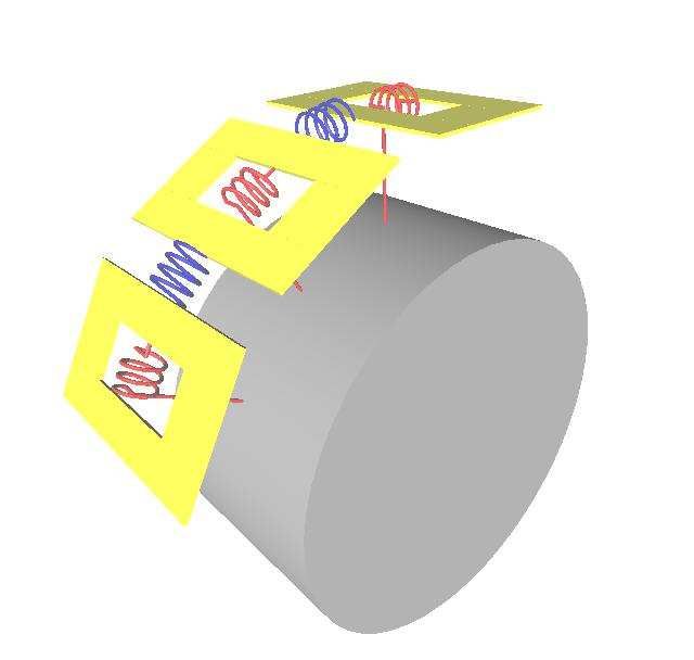
Contents

1 Legal Notices                                                                                                                                   1

2 Aims and Scope of FTire                                                                                                                         2

3 FTire Implementation and Interfaces                                                                                                             3

4 FTire Modelization                                                                                                                               4
  4.1 Mechanical Model . . . . . . . . . . . . . . . . . . . . . . . . . . . . . . . . . . . . . . . .                                        .    4
  4.2 Thermal Model . . . . . . . . . . . . . . . . . . . . . . . . . . . . . . . . . . . . . . . . .                                         .    5
       4.2.1 Thermal Model Structure . . . . . . . . . . . . . . . . . . . . . . . . . . . . . . . .                                          .    5
       4.2.2 Heat Generation and Heat Transfer Model . . . . . . . . . . . . . . . . . . . . . . .                                            .    5
       4.2.3 Determination of Heat Transfer Coefficients on Basis of Steady-State Temperatures                                                .    6
       4.2.4 Determination of Heat Capacities on Basis of Heating Time Constants . . . . . . . .                                              .    8
  4.3 Tread Wear Model . . . . . . . . . . . . . . . . . . . . . . . . . . . . . . . . . . . . . . . .                                        .    8
  4.4 Air Volume Vibration Model . . . . . . . . . . . . . . . . . . . . . . . . . . . . . . . . . .                                          .    9
  4.5 Flexible and Viscoplastic Rim Model . . . . . . . . . . . . . . . . . . . . . . . . . . . . . .                                         .   10

5 FTire Data                                                                                                                                      12
  5.1 Data Files . . . . . . . . . . . . . . . . . . . . . . . . . . . . . .          .   .   .   .   .   .   .   .   .   .   .   .   .   .   .   12
  5.2 Parameterization Process . . . . . . . . . . . . . . . . . . . . . .            .   .   .   .   .   .   .   .   .   .   .   .   .   .   .   12
       5.2.1 Preparation of the Identification Process . . . . . . . . . .            .   .   .   .   .   .   .   .   .   .   .   .   .   .   .   13
       5.2.2 Identification/Validation of Footprint Images . . . . . . .              .   .   .   .   .   .   .   .   .   .   .   .   .   .   .   13
       5.2.3 Identification/Validation of Static Properties . . . . . . . .           .   .   .   .   .   .   .   .   .   .   .   .   .   .   .   13
       5.2.4 Identification/Validation of Steady-State Rolling Properties             .   .   .   .   .   .   .   .   .   .   .   .   .   .   .   14
       5.2.5 Identification/Validation of Friction Characteristics . . . .            .   .   .   .   .   .   .   .   .   .   .   .   .   .   .   14
       5.2.6 Identification/Validation of Dynamic Cleat Tests . . . . .               .   .   .   .   .   .   .   .   .   .   .   .   .   .   .   14

6 FTire Parameter Specification                                                                                                                   16
  6.1 Scheme of tables . . . . . . . . . . . . . . . . . . . . . .    .   .   .   .   .   .   .   .   .   .   .   .   .   .   .   .   .   .   .   16
  6.2 Size, Geometry, Tire Specification, and Tread Pattern . . .     .   .   .   .   .   .   .   .   .   .   .   .   .   .   .   .   .   .   .   16
  6.3 Mass, Moments of Inertia, Inflation Pressure, and Volume .      .   .   .   .   .   .   .   .   .   .   .   .   .   .   .   .   .   .   .   22
  6.4 Structural Stiffness, Damping, and Hysteresis . . . . . . .     .   .   .   .   .   .   .   .   .   .   .   .   .   .   .   .   .   .   .   24
  6.5 Tread Geometry, Stiffness, Damping, and Friction . . . . .      .   .   .   .   .   .   .   .   .   .   .   .   .   .   .   .   .   .   .   37
  6.6 Temperature and Wear . . . . . . . . . . . . . . . . . . .      .   .   .   .   .   .   .   .   .   .   .   .   .   .   .   .   .   .   .   40
  6.7 Imperfections . . . . . . . . . . . . . . . . . . . . . . . .   .   .   .   .   .   .   .   .   .   .   .   .   .   .   .   .   .   .   .   41
  6.8 Misuse Data . . . . . . . . . . . . . . . . . . . . . . . . .   .   .   .   .   .   .   .   .   .   .   .   .   .   .   .   .   .   .   .   44
  6.9 Rim Data . . . . . . . . . . . . . . . . . . . . . . . . . .    .   .   .   .   .   .   .   .   .   .   .   .   .   .   .   .   .   .   .   44
  6.10 TPMS Sensor Data . . . . . . . . . . . . . . . . . . . . .     .   .   .   .   .   .   .   .   .   .   .   .   .   .   .   .   .   .   .   46
  6.11 Numerical Settings . . . . . . . . . . . . . . . . . . . . .   .   .   .   .   .   .   .   .   .   .   .   .   .   .   .   .   .   .   .   47

7 Operating Conditions                                                                                                                            50

8 Additional Runtime and Output Control                                                                                                           52

9 Undocumented Data Items                                                                                                                         62

10 TYDEX-Conform Output Signals                                                                                                                   64

11 Model Changes Log and Compatibility Mode                                                                                                       65

FTire Model Data                                                                                                                                  70

                                                     ii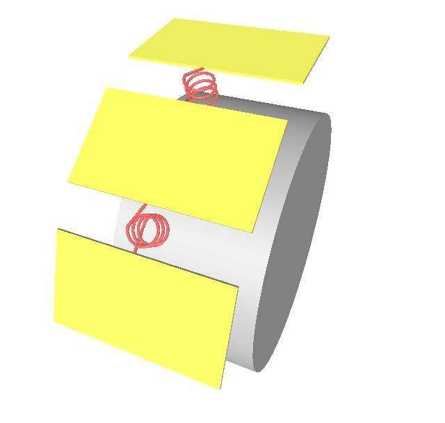
1 Legal Notices
This documentation is intended for qualified users who will exercise sound engineering judgment and expertise
in the use of the FTire software. The FTire software is inherently complex, and the explanations in this
documentation are not intended to be exhaustive or to apply to any particular situation. Users are cautioned
to satisfy themselves as to the accuracy and results of their analyses.
Cosin scientific software AG shall not be responsible for the accuracy or usefulness of any analysis performed
using the FTire software or the explanations in this documentation. Cosin scientific software AG shall not be
responsible for the consequences of any errors or omissions that may appear in this documentation.
The FTire software is available under license from cosin scientific software AG and may be used or reproduced
only in accordance with the terms of such license. This documentation is subject to the terms and conditions
of the then current software license agreement to which the documentation relates.
This documentation and the software described in this documentation are subject to change without prior
notice.
No part of this documentation may be reproduced or distributed in any form without prior written permission
of cosin scientific software AG.
The FTire software is a product of cosin scientific software AG, Muenchen, Germany.

                                                      1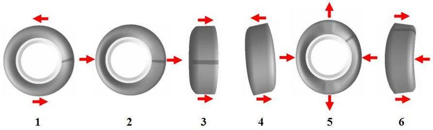
2 Aims and Scope of FTire
FTire (Flexible Structure Tire Model) is a full 3D nonlinear in-plane and out-of-plane tire simulation model. It
is used by engineers in the vehicle and tire industry worldwide. Sophisticated 2D and 3D rigid and flexible road
surface description models and evaluation methods, and powerful toolboxes for tire and road data processing
make FTire the most comprehensive software package for tire dynamics simulation on the market.
FTire is designed for vehicle comfort simulations and prediction of road loads on road irregularities even with
extremely short wave-lengths. It can also be used as a structural dynamics based, highly nonlinear and dynamic
tire model for handling studies without modifications of input parameters.
FTire explains most of the complex tire phenomena on a mechanical, thermodynamical, and tribological basis,
with very good correlation to measurements:
   • structural dynamics based, spatial nonlinear in-plane and out-of-plane tire model for simulation of belt
     dynamics, local contact patch pressure distribution, rolling resistance, side-wall contact, large camber
     angles and misuse scenarios;
   • suitable for a frequency range up to 200 Hz, excited by short surface wavelengths, mass imbalance,
     non-uniformity of tire and/or rim, air cavity vibrations, or irregular tread patterns;
   • very fast and flexible, up to real-time capability. Orders of magnitude faster than explicit FE models;
   • simulation of imbalances by inhomogeneous mass and stiffness distribution, radius variation, and local
     tread wear;
   • belt temperature distribution model;
   • air volume vibration model;
   • capability of tire slipping on rim for very large drive or brake torques;
   • integrated flexible and/or viscoplastic rim model;
   • support for user-defined wear, temperature distribution, and rim flexibility models;
   • full integration of cosin/road digital road library with support for complex rigid time-invariant and
     time-variant road surfaces;
   • full integration of cosin/soil digital road library with support for flexible and deformable road surfaces;
   • advanced online animation with belt deformation animation, tire temperature distribution animation,
     pressure distribution plots, road surface visualization and movie export;
   • robust, multi-core system enabled solver engine;
   • parameter editing and validation tools;
   • tailored parameter fitting tool (FTire/fit).

                                                       2
3 FTire Implementation and Interfaces
The FTire core library can be connected to all important simulation environments, by using cosin’s tire inter-
face (CTI), a C/C++ API. CTI provides a time-discrete generalized interface and reduces the implemen-
tation effort of FTire to a minimum. CTI is used by the FTire implementations in Adams (all variants), Mo-
tionSolve, SIMPACK, Abaqus, VI-CarRealTime, Matlab/Simulink, dSPACE-ASM, CarSim/TruckSim/BikeSim,
IPG Carmaker/Truckmaker, CASCaDE, cosin/mbs, DAFUL, Dymola/Modelica, FEDEM, Mesa Verde, PAM-
Crash, RecurDyn, veDyna, Virtual.Lab Motion, and others.
For Matlab/Simulink an S-function layer is available (FTire/link). This S-function is completed by a respec-
tive Simulink block-set.
All interfaces are designed to run an arbitrarily large number of tire instances simultaneously.
In either case, the coupling to the vehicle or suspension model of the calling program is done by the rigid
body state variables of the rim, that is:
   • position of the rim center in the inertial frame;
   • translational velocity vector of the rim center;
   • angular orientation of the rim, defined by the transformation matrix from the rim-fixed frame to the
     inertial frame. Euler angles, Cardan angles, or Euler parameters of the rim can be passed by an alternative
     API call. So the user can pass coordinates in the native reference frame of the calling application;
   • rotational velocity vector of the rim.
FTire returns forces and torques acting on the rim center, represented in the global coordinate system.
Alternatively, FTire can be used to simultaneously integrate the rim rotation with respect to the hub-carrier.
In this use mode, not the rigid-body states of the rim, but rather those of the wheel-carrier are the inputs,
together with the driving and the maximum absolute braking torque. The output torque vector then does not
contain the share in the direction of the wheel rotation. FTire eventually modulates the braking torque, if the
wheel is blocked, in order to maintain this blocking as long as it is necessary.

                                                         3
4 FTire Modelization
4.1 Mechanical Model
FTire is based on a structural dynamics based tire modeling approach.
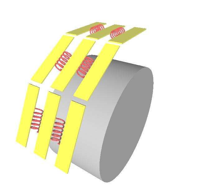
In this core mechanical model, the tire belt is described as an extensible and flexible ring, carrying bending
stiffnesses, elastically founded on the rim by distributed, partially dynamic stiffnesses in radial, tangential, and
lateral direction. The degrees of freedom of this ring are such that belt in-plane, as well as out-of-plane,
motions are possible. The ring is numerically approximated by a finite number of ’belt elements’. These belt
elements are coupled with their direct neighbors by stiff springs and by bending stiffnesses both in-plane and
out-of-plane.
All stiffnesses, bending stiffnesses, and damping factors are calculated during pre-processing, fitting the pre-
scribed modal and static properties (cf. list of data below).
To every belt element, a number (typically 5 to 50) of mass-less ‘tread blocks’ are associated. These blocks carry
nonlinear stiffness and damping properties in radial, tangential, and lateral direction. The radial deflections
of the blocks depend on the road profile, locus, and orientation of the associated belt elements. Tangential
and lateral deflections are determined by the sliding velocity on the ground and the local values of the sliding
coefficient. The latter depends on ground pressure and sliding velocity. ‘Radial’, ‘tangential’, and ‘lateral’ is
to be understood relatively to the orientation of the belt element, whereas ‘sliding velocity’ is the block end
point velocity, projected onto the road profile tangent plane. By polynomial interpolation, certain precautions
have been taken not to let the ground pressure distribution mirror the in-plane polygonal shape of the ‘belt
chain’.
To approximate reactions to out-of-plane excitations more accurately, every belt element has several additional
degrees of freedom. These degrees of freedom describe the element’s longitudinal rotation angle relative to
the rim, and the element’s bending in the lateral direction. The rotation angles are coupled by rotational
stiffnesses, located between two adjacent belt elements, as well as rotational stiffness for each belt element,
located between the belt elements and rim. At the same time, the coupling between the lateral displacement
of a belt element and its torsion angle is taken into account by an appropriate coupling stiffness.
The tread blocks, as mentioned above, are located along several parallel lines, such that both longitudinal and
lateral resolution of the road surface is optimized.
In unloaded condition, the belt elements are curvilinear in lateral direction. The actual curvature, however, is
not only determined by these geometrical values (which are defined by cross-section spline data), but at the
same time by the belt lateral bending degrees of freedom. The belt elements’ bending values, in turn, are
determined by the respective bending moments which are functions of the vertical forces of the belt elements’
tread blocks.
All 6 components of tire forces and torques acting on the rim are calculated by integrating the forces in the
elastic foundation of the belt.
The resulting overall tire model is accurate up to high frequencies, in both longitudinal and lateral direction.
There are few restrictions in the applicability w.r.t. longitudinal, lateral, and vertical vehicle dynamics situations.
FTire deals with large and/or short-waved obstacles. It works out of, and up to, complete stand still, with
no additional computing effort and without any model switch. Finally, it is applicable and accurate in more
delicate simulations such as ABS breaking on extremely uneven road surfaces, etc.
Optionally, FTire can take into account tire non-uniformity, which is a harmonic or more general variation of
the radial or tangential stiffness, as well as static and dynamic imbalances.
Kernel of the FTire implementation is an implicit integration algorithm that calculates the belt shape. By
using this specialized implicit BDF integrator, the belt extensibility may be chosen to be extremely small.
FTire thus also allows the simulation of an in-extensible belt without any numerical drawback.
44.2 Thermal Model
FTire provides an optional detailed thermal model, the foundations of which are described in this chapter.
This model is of special interest in case of strongly temperature-dependent friction properties. Activation and
deactivation is described in chapter8.
4.2.1 Thermal Model Structure
The FTire thermal model consists of the following components:
• the thermo-dynamical computation of the actual inflation pressure as function of air (or filling
gas) mass, ‘cold tire inflation pressure’, tire temperature, and actual interior volume. The tire filling gas
is considered to be ideal.
• a heat generation and transfer model, introducing state variables for the temperature of the tire
structure (including filling gas), and the individual temperature of each tread contact element. Heat
generation and transfer is driven by the power loss distribution due to structural damping and dry friction
on the road surface.
• the introduction of a third independent input variable ‘rubber temperature’ of the tread friction
characteristics, in addition to ground pressure and sliding velocity. This third independent variable is
taken into account in terms of a temperature-dependent correction factor of the friction coefficients:
µ = f (T ) · µ0 (v, pground )
4.2.2 Heat Generation and Heat Transfer Model
For simplicity, in the heat generation and transfer model, the tire is assumed to being separated into three
regions (figure 4.1), having different thermal properties each.
Figure 4.1: Regions of the thermal model
The following assumptions are made for the three different regions:
The tire structure is described by one global temperature only. The product of rate of change of this
temperature and the tire structure’s overall heat capacity is the balancing the sum of:
• the power lost in all damping elements in belt and side-wall, excluding friction and damping of the tread
elements.
• the heat which flows from the tire structure into the two tread regions. This heat transfer is determined
by the respective temperature differences, multiplied by an appropriate heat transfer coefficient. This
heat transfer coefficient is assumed to be independent on rolling speed.
• the heat which flows from the side-walls into the air flowing around the tire. This heat transfer is
determined by the temperature difference between tire structure and ambient air, multiplied by an ap-
propriate heat transfer coefficient. This heat transfer coefficient is assumed to be strongly and nonlinearly
dependent on rolling speed.
Document Revision: 2020-4-r23856
5The tread without contact patch is described by a distributed temperature, assigning one temperature
value individually to each tread element. The product of rate of change of this temperature and the tread
element’s heat capacity is balancing the sum of:
• the power lost in the tread element due to material damping.
• the share of the heat which flows from the tire structure into the particular tread element. This heat
transfer is the same as the already described heat transfer above.
• the heat which is transferred from the tread element to the air flowing around the tire. This heat
transfer is determined by the temperature difference between tread element and ambient air, multiplied
by an appropriate heat transfer coefficient. This heat transfer coefficient is assumed to be strongly and
nonlinearly dependent on rolling speed, but has the same value for all elements not in contact to the
road.
The contact patch is described by a distributed temperature, assigning one temperature value to each
individual tread element in the contact patch. The product of rate of change of this temperature and the
tread element’s heat capacity is balancing the sum of:
• a certain fraction △Pf rict, tread of the power lost in the tread element due to dry friction (the remaining
friction power is heating the road).
• the power lost in the tread element due to material damping.
• the share of the heat which flows from the tire structure into the particular tread element. This heat
transfer is the same as already described above.
• the heat which flows from the tread element into the road surface. This heat transfer is determined by
the temperature difference between tread elements and road surface, multiplied by an appropriate heat
transfer coefficient. This heat transfer coefficient is assumed to be independent of rolling speed, and
has the same value for all elements which are in contact with the road.
This model requires the following data:
• Heat capacity CS of the tire structure.
• Heat capacity CT of the tread; will be subdivided equally into the individual tread elements. The actual
tread depth is used to correct the actual heat capacity.
• Heat transfer coefficient κ (v) · cSE between the environment and the tire structure, assumed to be
dependent on rolling speed. This dependency is described by the factor κ (v).
• Heat transfer coefficient cST between the tread and the tire structure (will be subdivided equally into
the individual tread elements). This coefficient is assumed to be independent of the rolling speed.
• Heat transfer coefficient κ (v) · cT E between the environment and the tread, which is not in contact
with the road. This coefficient is assumed to dependent on the rolling speed of the tyre and is described
by the factor κ (v).
• Heat transfer coefficient cT R between the contact patch and the road surface (will be subdivided equally
into the individual tread elements). This coefficient is assumed to be independent of the tire rolling
speed.
To make data independent of the actual contact patch length, both values κ (v) · cT E and cT R are defined
as heat transfer coefficients per unit length, multiplied by the tire circumference.
The above data is proposed to be approximated by the following procedures.
4.2.3 Determination of Heat Transfer Coefficients on Basis of Steady-State
Temperatures
To determine the heat transfer coefficients, the following equations are used to describe the dependencies
of a given set of steady-state temperatures:
)
κi cSE · (TS,i − Tenv ) + cST · (TS,i − TT,i ) = 0
(i = 1, 2, . . .)
cST · (TT,i − TS,i ) + (λ cT R + (1 − λ) fi cT E ) · (TT,i − Tenv ) = PT.loss,i
Document Revision: 2020-4-r23856
6Here, index i denotes different rolling speeds at which the steady-state temperatures of the tread and eventually
the tire structure are assumed to being measured: v1 is 25% of vmax , v2 is 50% of vmax , and v3 = vmax .
λ is the relative share of the contact patch length to the rolling circumference at the assumed load (LI load,
say) where the measurements have been taken. Factors κi = κ (vi ) describe the dependency of the rolling
speed on the heat transfer due to the air-flow around the tire. The intention is to determine heat transfer
coefficients on the basis of measured steady-state temperatures as accurate, robust, and reliable as possible.
Several different approaches indicate that the following choice is a good compromise between accuracy and
robustness of identification:
cSE cST
• Choose α = cT E and β = cT R to be given a fixed number (1, say) that is not subjected to the
identification
• Normalize κ1 = 1 for an arbitrary reference rolling speed
• Use TS = TS,1 , TT = TT,1 and PT.loss = PT,loss,1 to determine and cT E and cT R
• For any arbitrary additional vi , use TT,i to determine κi
This leads to the following equations:
α cT E · (TS − Tenv ) + β cT R · (TS − TT ) = 0
β cT R · (TT − TS ) + (λ cT R + (1 − λ) cT E ) · (TT − Tenv ) = PT,loss
so
α (TS − Tenv ) β (TS − TT ) cT E 0
=
(1 − λ) (TT − Tenv ) β (TT − TS ) + λ (TT − Tenv ) cT R PT,loss
which can easily be resolved for cT E and cT R .
For any other rolling speed, it holds:
κi α cT E · Tenv + β cT R · TT,i
TS,i =
κi α cT E + β cT R
or
κi α cT E
TT,i − TS,i = (TT,i − Tenv )
κ i α cT E + β cT R
Substitute into the equation above:
κ i α cT E
β cT R · + λ cT R + (1 − λ) κi cT E · (TT,i − Tenv ) = PT,loss,i
κ i α cT E + β cT R
PT ,loss,i
After introducing the dimensionless variable γi = cT R (TT ,i − Tenv ) , and some rearrangements, one gets the
following quadratic equation for κi :
2
cT E β β γi − λ cT E β γi − λ
κi + + − κi − · = 0
cT R α 1−λ 1−λ cT R α 1−λ
which, due to the parameter ranges, will always have two real solutions. Moreover, one solution will be positive
and the other one negative, as long as:
γi PT,loss,i
= > 1
λ λ cT R (TT,i − Tenv )
meaning the amount of heat generated in the contact patch, due to friction, is greater than the heat being
transferred to the road in steady state conditions. This equation is used as a plausibility check for TT,i . In
any case, the solution of fi will be selected which is closer to +1.
As a matter of convenience, instead of TS,i , TT,i , the temperature increases △TS,i and ∆TT,i relative to
ambient temperature are to be provided as model data.
Document Revision: 2020-4-r23856
74.2.4 Determination of Heat Capacities on Basis of Heating Time Constants
To determine the heat capacities from the heating time constants, the following 2 differential equations, of
heat conduction at medium rolling speed, are used:
Cs ṪS,2 + f2 cSE · (TS,2 − Tenv ) + cST · (TS,2 − TT,2 ) = 0
CT ṪT,2 + cST · (TT,2 − TS,2 ) + (λ cT R + (1 − λ) f2 cT E ) · (TT,2 − Tenv ) = PT,loss,2
Here, for simplicity the assumption is made that tread temperature is constant along belt circumference. These
equations are governed by the 2x2 linear system matrix:
" #
− f2 cSECS+ cST cST
CS
A = cST
CT − λ cT R + (1 − C
λ) f2 cT E + cST
T
Using the following abbreviations: p = f2 cSE + cST , q = cST , r = λ cT R + (1 − λ) f2 cT E + cST ,
s = p r − q 2 , the (real) eigenvalues of this matrix are determined by:
λ1 + λ2 = tr (A) = − CpS − CrT = − r CCsS+CpTCT
λ1 λ2 = det (A) = CSsCT
Due to Ti = − λ1i , it follows r CS + p CT = −s λλ11+· λλ22 = s · (T1 + T2 ), therefore:
r CS + p CT = s · (T1 + T2 )
CS · CT = s · T1 · T2
The last equation finally leads to a quadratic equation for either of the two heat capacities, having the two
solutions:
q
(T1 + T2 ) ± 4sr2 (T1 + T2 )2 − ps
s 2
CS = 2r r T1 T2
CT = s TC1ST2
These two equations tell us how to compute the heat capacities from heating time constants. Unfortunately,
as a quadratic equation is underlying, they can have no, one or two solution(s). To get a unique approximation
in either case, the following rules are introduced:
• if the solution is complex, the ‘nearest’ real solution is taken, the parameters are thus given by:
CS = 2sr (T1 + T2 )
CT = s TC1ST2
• if the solution is real, select the solution so that CS > CT ;
• if the solution is real and CS > CT holds for both solutions, or for no solution, then the pair of heat
capacities is chosen for which |CS − CT | has the smallest value.
4.3 Tread Wear Model
For any tread element, the individual instantaneous power loss due to road friction is available as output of
the tire force model. Equally well, each tread element’s estimated instantaneous temperature is available
from the thermal sub-model.
The three variables: power loss Pf rict = |vslide | · |Ff riction |, temperature T , and tread-element’s normal
force FN are fed into a 3D characteristic, predicting the instantaneous tread block’s wear rate dhdt :
dh
= −f (Pf rict , T, FN )
dt
Document Revision: 2020-4-r23856
8This wear rate is integrated, resulting in a tread-block-individual state variable ‘tread element height h’. This
state has location-dependent values, distributed along the tire circumferential and lateral coordinates.
Besides merely calculating the wear rate, this state variable is used as time-dependent tread depth in the force
model. Thus, it affects the cross-sectional geometry, contact pressure distribution, radial tread stiffness, tread
shear stiffness, tire mass, and the tread’s heat capacity. Indirectly, tread wear affects the global tire stiffness
and handling properties. Moreover, because actual tread depth is a function of the tread element’s location
in the tread, tire imperfections like ‘spot wear’ etc. are subject to possible investigation.
The real challenge of this approach is to determine the wear function. This function f can only be approximated
on basis of appropriate measurements.
Starting point of the tread wear model is the following simple, two parameter, mathematical expression for f :
!ewear
dh Pf rict
= −cwear ·
dt 1 Nsm
These parameters, in turn, might be identified on basis of life-time tire wear properties. It is easy to connect
and use a user-defined expression instead. Activation and deactivation of the tread abrasion model is described
in chapter8.
4.4 Air Volume Vibration Model
FTire comes with an integrated optional air volume vibration model. This model describes fluctuations
of the air density, air pressure, and air flow velocity inside the tire, mainly caused by the cross sectional area
variations, due to the tire deflections of the rolling tire. Due to the unbalanced pressure reaction forces on
the rim and tire structure, as well as small pressure-dependent structural stiffness variations, these vibrations
might affect the overall tire forces in higher frequency ranges.
The following three equations establish the relationships between the air density ρ(t, x), air pressure p(t, x),
and air flow velocity u(t, x) in the circumferential direction. These relationships describe the one-dimensional
compressible air flow through the tire volume, driven by the time- and location-dependent cross section area
A (t, x):
• Impulse conservation:
∂ ∂ ∂p
Aρu2 = −A
(Aρu) +
∂t ∂x ∂t
• Mass conservation (equation of continuity):
∂ ∂
(Aρ) + (Aρu) = 0
∂t ∂x
• Adiabatic pressure/density relationship (for absolute pressure):
κ
p ρ
=
p0 ρ0
with initial and boundary conditions:
p(0, x) = p0
u(0, x) = 0
p(t, 2πrrim ) = p(t, 0)
u(t, 2πrrim ) = u(t, 0)
Document Revision: 2020-4-r23856
9These hyperbolic partial differential equations are timely and spatially discretized in accordance with the tire
structure discretization. By this, each belt segment carries two additional state variables: one for the pressure
fluctuation and one for the flow velocity. This system of ordinary differential equations, resulting from the
spatial discretization, is solved implicitly, synchronized with the solution of the belt’s structural equations of
motion.
The air volume vibration model does not consume much extra computational power, nor does it require any
extra parameters. Activation and deactivation is described in chapter 8.
4.5 Flexible and Viscoplastic Rim Model
Upon demand, FTire can replace the assumed rigid rim geometry by a more realistic flexible and/or viscoplastic
rim model. Activation and deactivation of this rim model is described in chapter 8.
The rim model, if activated, takes the distributed spatial forces, exerted by the tire structure on left and right
rim flange, and computes the resulting flexible and/or viscoplastic rim flange displacements and deformations.
Both force and displacement vectors are expressed in rim-fixed cylindrical coordinates, to take advantage of
any axisymmetric or pseudo-axisymmetric properties of the rim stiffness.
The computation of flexible displacement and/or plastic deformation can be done using either the internal
model or a user-written external model.
The internal model uses an approximating Green’s function of the rim stiffness. This function can be
viewed to be the result of a stiffness matrix condensation and inversion, assuming loads are only applied
in the discretized rim flange nodes, and expressing the resulting displacements in terms of the convolution
of the forces with Green’s function. FTire’s internal rim model takes into account both radial and lateral
displacements, but neglects circumferential displacements.
If the rim was perfectly axisymmetric (that is, all stiffness fluctuations caused by drillings, spokes etc. are
neglected) and if rim flange forces were all in the linear range (that is, no plasticity applies yet), a Green’s
function will exist and if will be independent of the circumferential position of the nodes on the rim flanges.
In this case, the stiffness condensation results in a simple relationship between the radial or lateral nodal
forces (one node per belt segment on either rim flange) fi (i = 0, .., nseg − 1) and the radial or lateral nodal
displacements di (i = 0, .., nseg − 1). For the sake of simplicity, we neglect:
• longitudinal forces/displacements;
• dependency of radial displacements on lateral or longitudinal forces;
• dependency of lateral displacements on radial or longitudinal forces;
• and any coupling between left and right rim flange.
With these simplifications, to be relaxed later, the following relationship holds, independently for lateral and
radial displacements/forces:
nseg /2
X
di = gk · fmod(i+k,nseg ) , i = 0, . . . , nseg − 1
k=−nseg /2
The weight factors, gk , are a discretization of the Green’s function, and can be determined through FEA, or
by processing respective load/deflection measurements. Typically, the weights will have a maximum at k = 0,
will rapidly decay with |k|, and will be symmetric: gk = g−k . The current implementation of the internal rim
model will approximately describes these weight factors with a single shape parameter, cf. chapter 8.
In most cases however, caused by spoke design, the rim can not be considered being perfectly axisymmetric.
In this case, Green’s function, and by this the weights gk , will depend on i as well. The current implementation,
of the internal rim model, assumes that this dependency approximately can be described by a higher order
harmonic stiffness modulation:
g0,k
gi,k =
1 + a · sin (nspokes · ϕi )
Document Revision: 2020-4-r23856
10i
where ϕi = 2π nseg , the number of rim spokes is denoted by nspokes , and a is a measure of higher order
harmonic stiffness fluctuation.
If the elastic deformations locally exceeds a certain threshold value, the rim will undergo permanent plastic
deformation, and only a part of the elastic deformation will be reversible. These thresholds, one for radial
and one for lateral displacement, are part of the model data. The permanent deformations, distributed along
the rim circumference, are separately saved for the left and right rim flanges and for the lateral and radial
directions, as part of the rim state array.
As an alternative to the internal model, FTire provides a straightforward program interface, to call a user-
written external model. The user provides this model in terms of a dynamic library, containing a C/C++
function with the following calling syntax:
void urim (
int ti , /* tire handle ( in ) */
int nseg , /* number of equally distributed nodes on one
rim flange ( in ) */
double rrim , /* rim bead radius [ m ] ( in ) */
double wrim , /* axial rim flanges distance [ m ] ( in ) */
double t, /* simulation time [ s ]. Terminate , if t >=1 e60 ( in ) */
double fl [][3] , /* force array on left rim flange nodes ,
in cylinder coordinates [ N ] ( in ) */
double fr [][3] , /* force array on right rim flange nodes ,
in cylinder coordinates [ N ] ( in ) */
double del [][3] , /* elastic displacements of left rim flange nodes ,
in cylinder coordinates [ m ] ( out ) */
double der [][3] , /* elastic displacements of right rim flange nodes ,
in cylinder coordinates [ m ] ( out ) */
double dpl [][3] , /* plastic deformation of left rim flange nodes ,
in cylinder coordinates [ m ] ( in / out ) */
double dpr [][3] , /* plastic displacements of right rim flange nodes ,
in cylinder coordinates [ m ] ( in / out ) */
int * ret , /* return code , 0= ok ( out ) */
char * file /* data file name ( in ) */
) {
/* add program code to compute del , der , dpl , dpr , and ret here */
}
Selection of the library, the module name within the library, and the data file is done with the CTI functions
ctiLoadRimModel() and ctiLoadRimData(); please refer to the CTI documentation for more information.
Default module name is urim(), default library name urim.dll or urim.so, respectively.
Document Revision: 2020-4-r23856
115 FTire Data
5.1 Data Files
All the FTire model data is contained in the FTire data-file. This data file is given either in TeimOrbit syntax,
with file-extension .tir, or in cosin/io syntax, with extension .ft. Examples of such FTire data files are
provided with the FTire distribution package.
The FTire model data, listed in such data files, is called basic parameters. These basic parameters are
processed during the initialization(called pre-processing), resulting in the preprocessed parameters. These
parameters are appended as binary data to the data file. Provided that the basic data has not changed, the
preprocessed data will be used in the next simulation run and thus skipping the pre-processing.
The CTI interface automatically recognizes whether several wheels of the car share the same basic data file.
In that case, pre-processing is done only once for all these files.
Data files might contain information which is not used by FTire itself, like data in the section [VERTICAL]
in the TeimOrbit files. Such information either is required by the calling solver environment, or is included for
compatibility with other tire models.
It is highly recommended not to edit data files directly, even if the file is saved in plain ASCII format. It is
recommended to use FTire/editor, which will always perform automatic consistency checks, prevent typos,
conveniently gives access to this documentation, and additionally lets you perform all kinds of visualizations,
analysis, and processing tasks complementary to simple editing.
5.2 Parameterization Process
A list of experimental data to parameterize FTire is proposed in the FTire Parameterization documentation.
Processing of these experimental datasets is best done by using FTire/fit, a tailored, user-friendly toolbox
for measurement-based parameterization of FTire. The fitting process, guided by FTire/fit, benefits from
certain known parameter sensitivities and physical properties of a tire model in general:
• usefulness of certain measurement types
• appropriate sequence in which measurements are evaluated
• appropriate sequence in which parameters are determined
• relevance of certain measurements for certain parameters
• plausible ranges of parameter values
• sensitivity between parameter values and model properties
One important, and recent, experience is about the role of modal data in the parameterization process. They
seem to contain less relevant information than static measurements (in contrast to what has been assumed in
the early days of FTire), and typically they are more laborious to obtain. There is one obvious cause for this
lack of relevant information: during the modal measurements, on an unloaded tire, only small amplitudes will
be reached. However, these measurements would then be used to parameterize a FTire model for load cases
with large to extreme deflection values, that is, for a completely different operating condition.
Another experience is the amount of valuable information contained in the footprint bitmaps. The same holds
for several kinds of static deflection curves, with and without camber angle, on a flat surface or on certain
well-defined obstacles. Moreover, handling properties, like cornering stiffness and pneumatic trail, show a high
correlation with certain out-of-plane stiffness data. In many cases, after a thorough analysis of static and
steady-state behavior, there remain only few dynamically relevant parameters to be adjusted in order to get a
good correlation for the dynamic cleat tests.
12The following procedure has been successfully used to parameterize a FTire model, and is well supported by
FTire/fit in all stages.
5.2.1 Preparation of the Identification Process
1. Create a new data file with FTire/estim (cf. figure 11), by specifying the tire and rim size, load
index, speed range, mass, and inflation pressure(s). As a reference tire, use one which is as close to the
new tire as possible. FTire/estim can be launched via the FTire/fit GUI, specify all drum diameters
and cleat geometries used during the identification and validation process. FTire/fit provides a set of
example road data files and functions to manage such obstacle-defining files.
2. Specify (’check-in’) all static, steady-state, and dynamic measurement files used in the sequel. If
these files are given in the TYDEX file format, a single mouse-click to check them in is sufficient in many
cases. FTire/fit will automatically recognize the kind of measurement they contain, will determine the
constant operating conditions like inflation pressure, wheel load, camber angle, etc., and will save the
information on how the validation or identification is to be performed. Moreover, depending on the kind
of measurement, it will occasionally extract relevant information like radial, longitudinal, lateral, and
torsional stiffness, cornering stiffness, slip stiffness, pneumatic trail, camber thrust, sliding friction, etc.,
and insert this information in terms of ’nominal data’ into the tire data file, or save it elsewhere. If the
files are given in any other ASCII format, FTire/fit will assist in importing these files and will create
TYDEX files out of them. If measurements are only given in terms of scanned images, FTire/fit also
provides a digitizing tool based on MSPaint, which also assists in creating TYDEX files.
3. Specify (’check-in’) all footprint bitmap files. FTire/fit will automatically calibrate these files and
save the relevant information for later validation.
4. Import or digitize the tread and carcass contour geometry data. FTire/fit provides a respective
digitizing tool.
5. Identify the dynamic rolling radius on the basis of the measurement of the angular velocity of a freely
rolling tire at different drum speeds and wheel loads (or roughly estimate the rolling radius by subtracting
the tread gauge from the maximum radius).
5.2.2 Identification/Validation of Footprint Images
1. Footprint size and shape at different wheel loads and camber angles. FTire/fit provides an automatic
simulation preparation tool and superimposes the simulated footprint boundary over the measured con-
tact patch bitmap. Again, all this is done by a single mouse-click. If there is a mismatch in size or shape,
adjust the in-plane and lateral bending stiffness.
5.2.3 Identification/Validation of Static Properties
• Vertical stiffness on a flat surface (which is merely a validation of the two deflection values for half
and full LI load that have been automatically inserted into the data file in step (5.2.1)). The respective
simulation has been prepared by FTire/fit; a single mouse-click is sufficient to launch the validation and
save all results for later report generation. If the actual stiffness deviates from the predicted one, adjust
the respective deflection values. This might happen if there is a discrepancy between the static and
the steady-state kind of simulation, caused by different treatment of hysteresis and friction properties,
longitudinal and lateral stiffness on a flat surface.
• Torsional stiffness (turning the standing tire about the vertical axis). Adjust the belt torsional stiffness
about radial axis accordingly, if the simulation deviates from the measurement.
• Vertical stiffness on a longitudinal and transversal cleat. Adjust the lateral belt bending stiffness
and the belt in-plane bending stiffness accordingly, if the simulation deviates from the measurement.
• Vertical stiffness at large camber angles on a flat surface and on a transversal cleat. Adjust the
belt torsion and twist stiffness about circumferential axis, if the simulation deviates from the measure-
ment.
• Longitudinal and lateral stiffness on flat surface. Adjust the longitudinal and lateral tire stiffness, if
the simulations deviate from the measurements.
Document Revision: 2020-4-r23856
135.2.4 Identification/Validation of Steady-State Rolling Properties
• Longitudinal slip stiffness. Either activate the measured nominal value directly, by replacing tread
rubber stiffness, or identify the tread rubber stiffness manually. Fire/fit has prepared the validation,
provided a respective measurement file is available.
• Cornering stiffness and pneumatic trail. Either activate the measured nominal values directly, by
replacing the lateral stiffness and out-of-plane bending stiffness, or (re-)identify these two values manually.
If there is a discrepancy to the value of the lateral stiffness as determined in section 5.2.3, find a
compromise.
5.2.5 Identification/Validation of Friction Characteristics
• Identify sliding friction coefficients. During check-in of the measurement files, FTire/fit has au-
tomatically collected all available and relevant cases. Ideally, this identification is performed by one
mouse-click only.
After the identification, validate the relevant measurement cases. These cases, which have been auto-
matically detected and collected by FTire/fit, include:
1. pulling the tire in longitudinal direction
2. pulling the tire in lateral direction
3. turning the tire about vertical axis
4. rolling at large longitudinal slip
5. rolling at large slip angle
If the identified values of stiction and sliding friction differ greatly, stick-slip-phenomena might occur
in the lateral and longitudinal stiffness simulations. In this case, find a compromise by relaxing the
differences of the friction coefficients.
5.2.6 Identification/Validation of Dynamic Cleat Tests
• Run a in-plane cleat-test identification (or just a validation), to determine the last few remaining
parameters like the percentage of free mass, the structural damping (expressed in terms of the modal
damping), longitudinal coupling of tread shear stiffness, tread rubber damping, etc.
• Run a out-of-plane cleat-test identification (or just a validation), to determine few more parameters
like conicity, modal out-of-plane damping, the coupling between belt torsion and lateral displacement,
etc.
In all the phases listed above, FTire/fit will automatically create diagrams showing the comparisons between
the simulation results and the corresponding measurement. Finally, with another mouse-click, FTire/fit
generates a comprehensive report file, containing all these comparisons and more.
Apparently, there are different combinations of parameters possible that all completely determine the structural
stiffness and damping properties of FTire. The choice of these parameters (irrespective of static, steady-state,
or modal nature) will depend on the kind of measurements that are available, or cost effective, or accurate
enough. Note that all the modal data is only used to determine the spring stiffnesses and damping coefficients,
such that the mathematical model, for small excitations, shows exactly the measured behavior in the frequency
domain. FTire is not a modal model, nor is it linear.
To facilitate the parameterization, a second tool (FTire/calc) is available, which calculates all static and
modal data used in FTire by means of a detailed FE model. In turn, this FE model only takes geometry
data and material properties of all tire components, like the carcass and belt layers, bead rubber, bead wire,
tread, and so on, as input. For those users that have access to these tire design data, the new approach might
become promising. In the end, it is planned to establish a CAE process chain that takes the tire design data
for the prediction, or at least rough estimation, of the tire handling and ride comfort characteristics.
The kernel of FTire/calc is a static version of the FE tire model FETire. Using the model, a list of relevant
load cases are automatically processed by FTire/calc, describing the tire deflections in several directions and
Document Revision: 2020-4-r23856
14magnitudes, as well as determining the natural frequencies and damping moduli of all relevant modes. The
whole process of estimating the structural stiffness data of FTire will take only a few minutes on a standard
PC.
Document Revision: 2020-4-r23856
156 FTire Parameter Specification
6.1 Scheme of tables
The meaning of all parameters in the main data section of a data file is described in the tables below. All
tables shown here follow the same scheme:
name in data file unit in unit in symbol or formula
data file TeimOrbit
data file
’software-friendly’ name (does not contain the physical Description Specification of a
blank spaces or special characters and is not unit as used of the units mathematical
case-sensitive) of the respective parameter, in data files in case of symbol or formula
exactly as it appears in the data file saved in TeimOrbit of the parameter,
cosin/io format data for use in the
format files, using subsequent
physical base description
quantities
such as time,
length,
force, mass,
and angle.
The actual
units of these
base
quantities are
defined in the
[UNITS]
section of the
data file.
6.2 Size, Geometry, Tire Specification, and Tread Pattern
name in data file unit in unit in symbol or formula
cosin/io TeimOrbit
data file data file
rolling_circumference mm length 2 π rbelt
This is the rolling circumference of the tire under normal running conditions, at small load (approximately
1/4 rated load) and low speed (≦1/5 rated speed). This parameter, if specified, is used to enhance the
tire-size-based belt radius estimation.
16name in data file unit in unit in symbol or formula
cosin/io TeimOrbit
data file data file
tire_section_width mm length wtire
This is the nominal maximum tire width, during inflated, but unloaded operating conditions. Typically, this
value is the first number in the tire dimension string.
name in data file unit in unit in symbol or formula
cosin/io TeimOrbit
data file data file
actual_tire_section_width mm length wtire,actual
This is the actually measured maximum tire width, during inflated, but unloaded operating conditions. By
default, actual tire width is the same as nominal tire width.
name in data file unit in unit in symbol or formula
cosin/io TeimOrbit
data file data file
tire_aspect_ratio % % atire
This is the percentage of tire height to tire width. Typically, this value is the second number in the tire
dimension string.
name in data file unit in unit in symbol or formula
cosin/io TeimOrbit
data file data file
rim_diameter inch length drim
This is the rim diameter. It is used to estimate the moment of inertia of the ‘non-vibrating’ parts of the
tire (those parts that are assumed to be fixed to the rim), as well as the maximum, possible, tire deflection.
Typically, this value is the third number in the tire dimension string.
name in data file unit in unit in symbol or formula
cosin/io TeimOrbit
data file data file
rim_contour string string in RCL
quotes
rim_width inch length wrim
wheel_offset_ET mm length ET
These two parameters describe the basic rim geometry.
• wrim is the rim width (distance between the two rim flanges). Among others, it is used as the default
value for the belt width, in determining potential rim-to-road contact, and for the computation of FTire’s
Document Revision: 2020-4-r23856
17animation model.
• ET (German for ’Einpresstiefe’) is the optional wheel offset (distance between rim mid-plane and rim
mounting plane). ET is positive if rim mid-plane is closer to the vehicle’s center-plane than the rim
mounting plane, and negative if not.
• RCL is the rim contour letter as defined and used in ETRTO, currently one out of J, JJ, B, W, DW,
TW. Default is J. The rim contour letter mainly specifies certain standardized geometrical values like
rim flanges height and width, etc.
name in data file unit in unit in symbol or formula
cosin/io TeimOrbit
data file data file
load_index integer integer LI
speed_symbol string string in SS
quotes
intended_use string string in u
quotes
These three parameters are the standardized codes for the tire’s load capacity, maximum speed, and (optional)
intended tire use.
• The load index LI ranges from 19 (which means 77kg max. load) to 204 (which means 16000kg max.
load). Any value larger than 204 is assumed to be the maximum load in [kg].
• The speed symbol ranges from ‘A1’ (= 5 km km km
h ) to ‘Y’ (= 300 h ) and ‘ZR’ (maximum speed 240 h and
above). Any other numerical value (enclosed with quotes) is assumed to mean the encoded maximum
speed in [ km
h ].
• The intended use symbol u is either blank (default), or P (p-metric), LT (light truck), ST (special trailor
service), T (temporary spare), or C (commercial).
name in data file unit in unit in symbol or formula
cosin/io TeimOrbit
data file data file
belt_width mm length wbelt
tread_width mm length wtread
wbelt is the width of the belt. This parameter is needed to determine the effective belt shape, under lateral
bending, and other auxiliary stiffness values.
wtread is the maximum width of the tread that might come into contact with the road surface under extreme
running conditions. Among others, it is needed to determine the width of the belt element strips. Moreover, it
influences the computation of the longitudinal and lateral stiffness of the discrete tread blocks, that represent
the stiffness of the tread area. For this, the following relationships hold:
P △A
cradial = E
100 h
and
1
ctangential = cradial
3
where
2 π rbelt wtread
△A =
nseg nblocks
Document Revision: 2020-4-r23856
18h = dtread + dtread,0
N
E = E(S) = 10a
m2
a = 5.33905 + 0.020477 · S
and
P % of positive tread,
rbelt belt radius if tire is not inflated and not loaded, at zero speed,
nseg number of belt segments
nblocks number of contact points per segment
dtread tread depth
dtread,0 rubber height over steel belt, at zero tread depth
S Shore-A hardness of tread rubber, under the operating conditions
the model will be used in
name in data file unit in cosin/io unit in TeimOrbit symbol
data file data file or
formula
tread_pattern_file string string in quotes
tread_pattern_xmin 0.0 .. 1.0 0.0 .. 1.0 xmin
tread_pattern_xmax 0.0 .. 1.0 0.0 .. 1.0 xmax
tread_pattern_ymin 0.0 .. 1.0 0.0 .. 1.0 ymin
tread_pattern_ymax 0.0 .. 1.0 0.0 .. 1.0 ymax
tread_pattern_variation % % sT P
The first parameter is the name of a b/w bitmap file which shows all or part of the tread pattern. This file is
optional. If specified, it is used by FTire to compute the contact elements height accordingly. In doing so, the
actual tire’s tread pattern will be roughly approximated by FTire. Clearly, the accuracy of this approximation
depends very much on the number of contact points, and will thus be limited.
Usage of this option is meant mainly for the modelization of tires with relatively large blocks and/or
grooves.
The file format of the bitmap file must be bmp; file extension is expected to be ‘.bmp’. You might wish to use
an image processing software (like GNU Gimp, Mac OS X Paintbrush, Microsoft Paint, Google Picasa, Adobe
PhotoShop or any other), to import other image formats like png, tiff, or jpg.
The bitmap file is to be given in one of the standard resolutions (1, 4, 8, 16, 24, or 32 bits per pixel). FTire
assumes that the part of the tread which comes into contact to the road is shown in black color, while groves
appear in white color. Grayscale bitmaps may be used as well, to define a relative tread thickness. Tread
element heights are set according to the local brightness. As with purely b/w bitmaps, ‘black’ means maximal
thickness and ‘white’ means groove or void. Colored bitmaps can be used as well, even if not recommended;
only the pixels’ brightness will be used.
The bitmap file will automatically be scaled by FTire in such a way that the width of the file exactly covers the
tread width of the FTire model. Moreover, scaling factor in circumferential direction is the same as scaling
factor in lateral direction. This kind of scaling ensures there will be no distortion of the approximated tread
pattern. If the file does not show the total circumference (normally, it will not), it will be periodically repeated
to cover the full length of the tread.
By choosing a ‘bounding box’, defined by xmin , xmax , ymin , ymax , a certain part of the bitmap can be
selected to be repeated periodically in x- and/or y-direction. These parameters are optional. Default value
Document Revision: 2020-4-r23856
19for xmin and ymin is 0.0 (left or lower boundary, respectively); default value for xmax and ymax is 1.0 (right
or upper boundary, respectively).
sT P denotes an optional standard deviation of the tread pattern repetition length in case of tread pattern
specification by a bitmap file. Such a stochastic unequal spacing is usually applied to reduce peaks in the
rolling noise spectrum.
name in data file unit in unit in symbol
cosin/io TeimOrbit
data file data file
tread_pattern_geometry string string in
quotes
This string variable will define a special tread pattern geometry, and is an alternative to defining the tread
pattern by a bitmap file. It starts with a keyword, defining the kind of geometry, followed by a list of additional
numerical values. At present, the following special kind of geometries are supported:
• ‘grooves n w p1 p2 . . . pn ’ will define a set of n longitudinal grooves, each with width w [mm]. The
position of the i-th groove center relative to tread width is given by the percentage pi . For example,
‘grooves 2 8 50 75’ will define two 8 mm grooves, one at the tread center and another one in the
middle between tread center and right-hand side tread end. For reasons of numerical accuracy, if defining
grooves, the number of tread strips (nstrips ) should be set large enough. In most cases, 50 tread strips
will be sufficient.
• ‘rib_edges q1 q2 . . . qn ’ will define a set of n − 1 longitudinal grooves. Position and width of groove #
i is defined through absolute distances from the tread center line with the numbers q2i−1 and q2i [mm].
For reasons of numerical accuracy, if defining grooves, the number of tread strips (nstrips ) should be
set large enough. In most cases, 50 tread strips will be sufficient.
name in data file unit in unit in symbol or formula
cosin/io TeimOrbit
data file data file
belt_lat_curvature_radius mm length rbelt,lat
rel_tread_shoulder_width % % wshoulder,rel
rel_min_tread_shoulder_height % % hshoulder,rel,min
belt_layers_thickness mm length hbelt
inner_liner_thickness mm length hil
These variables describe the geometrical shape of the tread surface and other cross-section data.
• rbelt,lat denotes the curvature of the outermost belt layer in lateral direction (that is, perpendicular to
the rim mid-plane). The tire is in inflated, but unloaded condition. This radius influences the ground
pressure distribution in the contact patch, and thus, most of all, the shape of the contact patch, and
the aligning torque.
• wshoulder,rel is the width of one tread shoulder relative to the tread width. The tread depth is assumed
to vary in a smooth quadratic way between maximum height at the inner start of the tread shoulder,
and a final value at the outer end of the shoulder, which coincides with the tread end.
• hshoulder,rel,min is the tread depth at the outer end of the shoulder, measured relative to the maximum
tread depth
• hbelt is the mean height of all belt layers
• hil is the mean height of the tire inner-liner
Document Revision: 2020-4-r23856
20You can also read