Country-resolved combined emission and socio-economic pathways based on the Representative Concentration Pathway (RCP) and Shared Socio-Economic ...
←
→
Page content transcription
If your browser does not render page correctly, please read the page content below
Earth Syst. Sci. Data, 13, 1005–1040, 2021
https://doi.org/10.5194/essd-13-1005-2021
© Author(s) 2021. This work is distributed under
the Creative Commons Attribution 4.0 License.

                       Country-resolved combined emission and
                        socio-economic pathways based on the
                         Representative Concentration Pathway
                          (RCP) and Shared Socio-Economic
                               Pathway (SSP) scenarios
                Johannes Gütschow1 , M. Louise Jeffery1,3 , Annika Günther1 , and Malte Meinshausen2
                      1 PotsdamInstitute for Climate Impact Research, Telegrafenberg, Potsdam, Germany
         2 Climate   & Energy College, School of Earth Sciences, The University of Melbourne, Melbourne, Australia
                                            3 NewClimate Institute, Berlin, Germany

                        Correspondence: Johannes Gütschow (johannes.guetschow@pik-potsdam.de)

                                       Received: 22 April 2020 – Discussion started: 4 June 2020
                          Revised: 28 January 2021 – Accepted: 31 January 2021 – Published: 11 March 2021

       Abstract. Climate policy analysis needs reference scenarios to assess emission targets and current trends. When
       presenting their national climate policies, countries often showcase their target trajectories against fictitious so-
       called baselines. These counterfactual scenarios are meant to present future greenhouse gas (GHG) emissions in
       the absence of climate policy. These so-called baselines presented by countries are often of limited use, as they
       can be exaggerated and as the methodology used to derive them is usually not transparent. Scenarios created by
       independent modeling groups using integrated assessment models (IAMs) can provide different interpretations
       of several socio-economic storylines and can provide a more realistic backdrop against which the projected
       target emission trajectory can be assessed. However, the IAMs are limited in regional resolution. This resolution
       is further reduced in intercomparison studies, as data for a common set of regions are produced by aggregating
       the underlying smaller regions. Thus, the data are not readily available for country-specific policy analysis. This
       gap is closed by downscaling regional IAM scenarios to the country level. The last of such efforts has been
       performed for the SRES (“Special Report on Emissions Scenarios”) scenarios, which are over a decade old
       by now. CMIP6 (Coupled Model Intercomparison Project phase 6) scenarios have been downscaled to a grid;
       however they cover only a few combinations of forcing levels and SSP storylines with only a single model per
       combination. Here, we provide up-to-date country scenarios, downscaled from the full RCP (Representative
       Concentration Pathway) and SSP (Shared Socio-Economic Pathway) scenario databases, using results from the
       SSP GDP (gross domestic product) country model results as drivers for the downscaling process. The data are
       available at https://doi.org/10.5281/zenodo.3638137 (Gütschow et al., 2020).

1   Introduction                                                    of emissions as well as socio-economic storylines to enable
                                                                    cross-comparison of a wide range of mitigation, adaptation,
In order to coordinate climate change research, different sets      and climate change impact studies (Nakicenovic and Swart,
of joint scenarios have been developed. For example, the In-        2000; Riahi et al., 2007). These “marker scenarios are no
tergovernmental Panel on Climate Change (IPCC) “Special             more or less likely than any other scenarios but are consid-
Report on Emissions Scenarios” (SRES) summarized avail-             ered by the SRES writing team as illustrative of a particular
able literature and provided six illustrative marker scenarios      storyline” (Nakicenovic et al., 2000). More recently a new

Published by Copernicus Publications.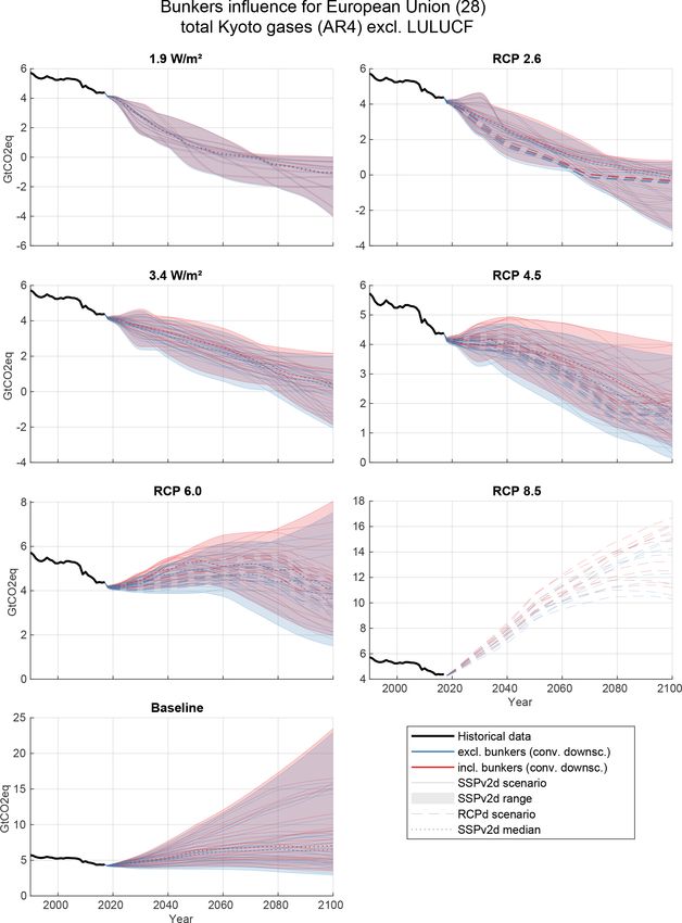
1006                                            J. Gütschow et al.: Country pathways based on the RCP and SSP scenarios

scenario process was started (Moss et al., 2010). The emis-        been very limited compared to those categorized as Annex I
sion scenarios used in that process are the Representative         (industrialized) countries.
Concentration Pathways (RCPs) that have been developed                 This limitation of country-level detail can severely ham-
on the basis of four harmonized emission scenarios from dif-       per a number of studies: climate impact assessments, quan-
ferent integrated assessment model (IAM) modeling groups           tification of equity principles for effort sharing of mitigation,
(van Vuuren et al., 2011a; Meinshausen et al., 2011; van Vu-       or the assessment of pledges of countries against benchmark
uren et al., 2011b; Thomson et al., 2011; Masui et al., 2011;      reference and mitigation scenarios. The required long-term
Riahi et al., 2011).                                               country-level scenarios are only available based on the SRES
   In a second step following the selection of concentration–      scenarios that are now over a decade old (van Vuuren et al.,
emission scenarios, five different socio-economic story-           2007; Höhne et al., 2010).
lines were developed, the Shared Socio-Economic Pathways               Sector and gas resolution is limited as well. While the
(SSPs; Nakicenovic et al., 2014), allowing for mitigation and      RCP scenarios have detailed sectoral data for some gases
impact researchers to combine low- and high-emission fu-           (e.g., CH4 ), the resolution of CO2 is limited to separating
tures with different assumptions about socio-economic de-          land use emissions from the fossil fuel and industrial emis-
velopment in terms of population, gross domestic product           sions in the publicly available database. The shared SSPv2
(GDP), and further indicators (van Vuuren et al., 2014). This      IAM outputs only resolve between land use and fossil fuel
is an advancement over the SRES scenarios, as in the SRES          and industrial emissions, and hence also coarse disaggrega-
scenarios, an emission future was often assumed to be in           tion is harmonized towards common historical emission lev-
line with a single socio-economic development only. The ex-        els. The RCPs resolve individual fluorinated gases, while the
ception during the SRES scenario process was the A1 sce-           SSPv2 database only provides data for aggregated fluorinated
nario family that was during the plenary adoption process          gases.
split out into three sub-scenarios, A1FI, A1T, and A1B, in-            Recently, the scenarios for the Coupled Model Intercom-
dicating the importance of socio-economic assumptions be-          parison Project phase 6 (CMIP6; World Climate Research
low the high-level “high-growth” storyline of the A1 family        Programme, 2019) have been released so that they are also
and their respective effect on emissions. The new SSP socio-       based on the RCP forcing levels and SSP storylines. They
economic storylines were modeled by several independent            provide socio-economic and emission data on a more de-
groups to quantify them in terms of GDP (Leimbach et al.,          tailed regional, gas, and categorical level. Even though data
2017; Dellink et al., 2017; Crespo Cuaresma, 2017), pop-           exist that are downscaled to a grid – with an intermediate step
ulation (KC and Lutz, 2017), and urbanization (Jiang and           of downscaling to the country level (Gidden et al., 2019) –
O’Neill, 2017) development on a country or detailed regional       there are no country-resolved data available. Transformation
level. These scenario quantifications are called the SSP basic     of gridded data to the country level is problematic for small
elements.                                                          countries unless the grid is very fine. Furthermore, only a few
   As a further step in this process, several research             combinations of RCP forcings with SSP storylines each from
groups used IAMs to simulate combinations of the Shared            a single model only are included in the SSP CMIP6 database
Socio-Economic Pathways with Representative Concentra-             (IIASA, 2018; Gidden et al., 2019; Feng et al., 2020).
tion Pathway forcing targets (Riahi et al., 2017; Kriegler             To fill this gap and provide country-level data for all RCP–
et al., 2017; Fujimori et al., 2017; Calvin et al., 2017; Fricko   SSP combinations and IAMs, we downscale the RCPs and
et al., 2017; van Vuuren et al., 2017; Rogelj et al., 2018).       SSPv2 emission scenarios to the country level using the SSP-
   While the IAMs internally use between 11 and 26 re-             basic-elements socio-economic country-level data. To down-
gions, the published data are limited to a set of macro re-        scale the RCPs we use per country GDP results from all three
gions, namely the RC5 regions (RC: region categorization;          groups provided in SSP-basic-elements GDP scenarios. Our
see Appendix II.2.2 of Edenhofer et al., 2014) for the RCPs        data thus enable a comparison of results between SSP-basic-
and the RC5.2 regions (IIASA, 2016) for the SSPs. The rea-         elements modeling groups and IAMs and provide ranges for
sons for this limitation are manifold: decisions of the inter-     future country emissions under different SSP storylines and
comparison protocols allowing for a wide participation of          RCP forcing targets instead of the seeming certainty given
modeling groups lead to a neglect of some regional detail,         by the single model used in the SSP CMIP6 data.
but more fundamentally, the quality of calibration and input           Historical emission data are taken from the PRIMAP-hist
data for the global modeling exercises that produced the SSP       v2.1 (Potsdam Real-time Integrated Model for the proba-
GDP and population projections degrades on finer scales and        bilistic Assessment of emission Paths) source, which pro-
hence limits the projection models. Furthermore, so far there      vides data for all countries and Kyoto greenhouse gases (Ky-
are no official and comprehensive emission inventories for         oto GHGs) (Gütschow et al., 2016, 2019) based on offi-
most countries that are categorized as non-Annex I countries,      cial UNFCCC data complemented by third-party data to fill
as their reporting requirements under the UNFCCC (United           the reporting gaps for non-Annex I countries and years be-
Nations Framework Convention on Climate Change) have               fore 1990. Historical socio-economic data are taken from
                                                                   Gütschow (2019), which is based on UN population data

Earth Syst. Sci. Data, 13, 1005–1040, 2021                                         https://doi.org/10.5194/essd-13-1005-2021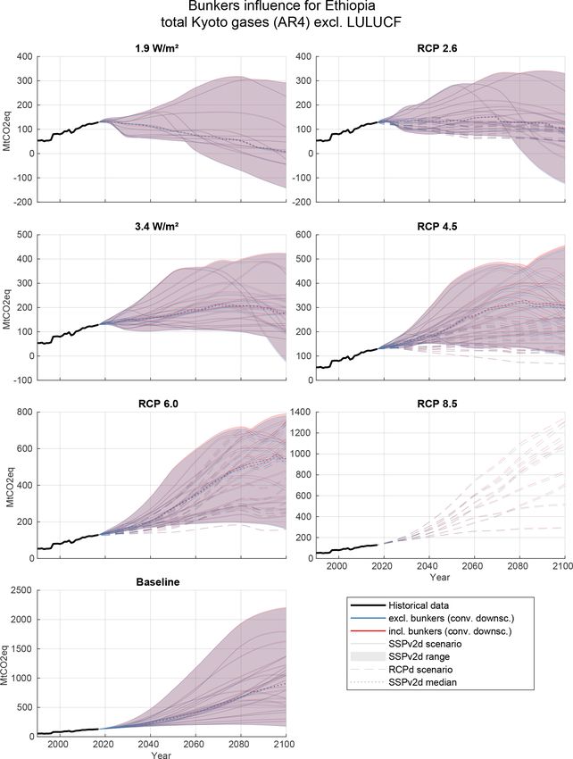
J. Gütschow et al.: Country pathways based on the RCP and SSP scenarios                                                     1007

(UN DESA/Population Division, 2019) and the Maddison               2.2   Existing downscaling methods
Project database (Bolt et al., 2018a, b) as well as other
                                                                   Several methods to downscale emission data are found in
sources to fill missing values. Our downscaling methodology
                                                                   the literature. Which methods can be used depends on avail-
is based on existing approaches, which we extend and im-
                                                                   able data and the choice between a simple and transparent
prove to enable its use on scenarios with negative emissions.
                                                                   method versus a more realistic but also more complex ap-
   The paper is structured as follows: we begin with the
                                                                   proach. Common to all methods is the need for an auxiliary
review of existing downscaling methodologies and the in-
                                                                   dataset called the downscaling key. Data from the downscal-
troduction of our methodology in Sect. 2. In the following
                                                                   ing key are used directly or as the basis for a model to split
Sect. 3 we describe the data sources this work is based on and
                                                                   the regional data to the country level. It could be data for
how they are processed. Section 4 presents a detailed step-
                                                                   the same variable from a different source or for a different
by-step description of our downscaling approach. Results are
                                                                   variable with some known or assumed correlation to the vari-
presented in Sect. 5, followed by a discussion of limitations
                                                                   able that is to be downscaled. The data can either cover the
(Sect. 6) and conclusions (Sect. 8). The availability of the re-
                                                                   same period of time, historical years only, or even a single
sulting datasets is described in Sect. 7. The Appendix gives
                                                                   year only. The basis of our work is the three groups of meth-
details on the data sources for the historical socio-economic
                                                                   ods identified in van Vuuren et al. (2007), which differ in
data, data coverage of the different scenarios, and additional
                                                                   their use of the downscaling key. They specifically consider
methodological details. The Appendix also provides tables
                                                                   cases where country-resolved emission data are available up
with acronyms and definitions used throughout this paper.
                                                                   to a certain year but future projections are only available for
                                                                   larger regions, as this is the situation given by the combina-
2     Methods                                                      tion of RCP scenarios with the SSP-basic-elements and the
                                                                   SSPv2 IAM runs.
2.1    Notation
In the following we consistently assume data are given for a         – Linear downscaling. This is the simplest method. The
region R, which we describe as a set of countries C ∈ R. We            downscaling key is a dataset for the same variable as
denote this by subscript identifiers. A regional emission path-        the to-be-downscaled data, e.g., both CO2 emissions.
way is denoted by ER ; an emission pathway for a specific              Historical emission data for one single year y0 (or
country C is denoted by EC . Emissions for a specific year y           an averaged period) is used to define shares SC (y0 ) =
are denoted by ER (y) or EC (y) respectively. We denote emis-          EC (y0 )/ER (y0 ) for each country C ∈ R. These shares
sion intensity by EI, GDP by GDP, and population by POP                SC (y0 ) are used to distribute emissions from the regional
in a similar way. For calculations with full pathways we as-           pathway to individual countries: EC = SC (y0 )ER . The
sume that the same operation is applied on data points for all         relative emissions of countries within a region are thus
years individually; i.e., EI · GDP denotes the multiplication          fixed at the historical level for the whole resulting sce-
of emission intensity by GDP for each year. EI · GDP(y) de-            nario. This approach was used by the MATCH group
notes the multiplication of the whole emission intensity time          (Modeling and Assessment of Contributions to Climate
series by the GDP of year y. Emissions and emission inten-             Change UNFCCC ad hoc group; Höhne et al., 2010) to
sities are defined for several variables (gases and pollutants),       downscale SRES scenarios from the region to country
but as we are only working on one gas at a time, we do not             level.
introduce another subscript index for these variables for the            While this approach is very transparent and straight for-
sake of a simpler notation. The method could as well be used             ward, it has the downside that it can not model differing
to downscale the world to the regional level or country emis-            developments within a region. All countries in a region
sions to the state level. We only consider downscaling from              will have the same emission growth rates defined by the
larger to smaller economic or political regions, e.g., from the          regional pathway. The method is likely to overestimate
region level to the country level, and do not consider spatial           future emissions of relatively developed countries com-
downscaling of data from coarser to finer grids. However, if,            pared to those of developing countries with high eco-
e.g., GDP data are given on a finer grid than emission data,             nomic growth within the same region. See also results
the method described here could also be applied.                         Sect. 5.
   We denote the RCP scenarios and forcing levels as RCP
and the downscaled RCP scenarios as RCPd. The SSP basic              – External-input-based downscaling. In this method a
elements are abbreviated as SSPbe. With SSPv2 we denote                country-resolved key pathway KC for some variable
the SSP IAM scenarios version 2, and with SSPv2d we de-                is available. The shares SC = KC /KR defined by this
note the downscaled SSPv2 scenarios. When using just SSP               pathway are used to downscale the regional pathway:
we refer to the SSP storylines; e.g., RCP–SSP refers to the            EC = SC ER .
combination of RCP forcing levels with SSP storylines.                   This method can take different developments within the
                                                                         region into account but only to the extent the down-

https://doi.org/10.5194/essd-13-1005-2021                                         Earth Syst. Sci. Data, 13, 1005–1040, 2021
1008                                           J. Gütschow et al.: Country pathways based on the RCP and SSP scenarios

    scaling key data K does itself. The intra-regional dif-          Figure 1 shows examples for the three methods described
    ferentiation will be that of the existing key source, only    above.
    scaled with the ratio of the regional scenario pathway to        Which method is most appropriate depends on the in-
    the regional key pathway. If the key data for a different     tended use and available data. If only historical data are avail-
    variable than the regional data are to be downscaled, a       able, linear downscaling is often the only method that can
    systematic error is introduced if the two variables are       be used to derive country-level future emissions from re-
    not linearly correlated. If the correlation is known, this    gional emission projections. Convergence downscaling is a
    might be compensated, but in general this will not be         good option, if the variable that should be downscaled can be
    the case. We use this method to downscale the SSPv2           expressed relative to some known variable to make it com-
    socio-economic data and the PIK (Potsdam Institute for        parable between different countries, which is a prerequisite
    Climate Impact Research) SSPbe data from the region           for the convergence concept to be meaningful. If emission
    to country level.                                             data are available from a different source, the external-input
                                                                  method is a good option.
  – Convergence downscaling. Convergence downscaling                 For our task we use a slightly modified version of the
    uses the assumption that a given variable converges           convergence downscaling which can handle negative emis-
    among countries within a given region. The conver-            sions and uses the GDP data provided by the SSP basic el-
    gence assumption only makes sense for variables which         ements and the IPAT equation (described below) to down-
    are independent of the size of a country, e.g., emis-         scale the emissions of the greenhouse gases included in the
    sion intensity (emissions per unit of GDP) and GDP per        RCP and SSPv2 scenarios. Our method is very similar to
    capita but not absolute emissions or GDP. This method         the convergence downscaling employed in van Vuuren et al.
    needs historical information for the target variable (e.g.,   (2006, 2007) (see Sect. 2.3).
    emissions), and in the case that the target variable is not
    independent of country size an auxiliary variable that
                                                                  2.3   IPAT convergence downscaling
    can be used to create a convergence variable which does
    not depend on country size (e.g., GDP to create emis-         In this section we present the details of our modified ver-
    sion intensity). Furthermore, regional and country time       sion of the IPAT-based convergence downscaling introduced
    series for the auxiliary variable are needed for the full     in van Vuuren et al. (2006, 2007).
    downscaling period.                                              Similar to the original approach the basis for the down-
    The downscaling process begins with the creation of a         scaling of emissions is given by the IPAT equation (Ehrlich
    temporary pathway of the convergence variable for all         and Holdren, 1971; Chertow, 2000):
    countries, starting from the historical values for each
                                                                  I = P ·A·T.                                                  (1)
    country and ending at a common value obtained from
    the given regional pathway. Thus, all countries con-          The idea behind the equation is to decompose an environ-
    verge to the regional value in the convergence year. The      mental impact I into its drivers. The IPAT equation assumes
    convergence year can be set depending on the scenario         I is linear in all three drivers: the population size P , the af-
    storyline and governs if full or partial convergence is       fluence A as a measure of consumption of goods per capita,
    achieved within the scenario timeframe. To accomplish         and a technology factor T which governs the environmental
    partial convergence, the convergence year is set after the    impact per unit of consumed goods. In our case the envi-
    end of the scenario timeframe, and thus some form of          ronmental impacts to be described are greenhouse gas emis-
    extrapolation of the regional data is needed. In the case     sions. As we work on an economy-wide level the affluence
    that we used an auxiliary variable we need to multiply        is described by GDP per capita, and the emission intensity of
    the obtained pathways by the pathways of the auxiliary        the GDP plays the role of the technology factor. The driver
    variable to obtain the temporary pathways for the down-       behind emission growth is total GDP (as a measure of con-
    scaling variable. The obtained temporary pathways are         sumption and production), not the size of the population.
    scaled such that their sum matches the regional pathway          Our IPAT equation variant thus becomes
    prescribed by the scenario for every year individually.
                                                                               GDPC EC
    Convergence downscaling was employed by van Vu-               EC = POPC              = GDPC · EIC ,                        (2)
    uren et al. (2006, 2007) to downscale the SRES scenar-                     POPC GDPC
    ios from the region to country level.                         where EIC = EC /GDPC is the emission intensity of country
    This method employs socio-economic scenarios as the           C, the emissions per unit of GDP. The downscaling is carried
    drivers of the downscaling process and is therefore a         out individually for each gas g (index omitted).
    promising candidate to downscale the RCP and SSPv2               Figure 2 gives an overview of the steps of the downscaling
    scenarios using the SSP-basic-elements country-level          process, which will be described in detail in the following
    data. Details are presented in Sect. 2.3.                     sections.

Earth Syst. Sci. Data, 13, 1005–1040, 2021                                        https://doi.org/10.5194/essd-13-1005-2021
J. Gütschow et al.: Country pathways based on the RCP and SSP scenarios                                                                  1009

Figure 1. Example results for different downscaling approaches. For the sake of simplicity a two-country region is assumed. The constant-
relative-emission-intensity downscaling is a variation of the external-input-based downscaling, where we use GDP as external input, and the
assumption of constant relative emission intensities to create emission pathways based on the GDP data (b). Regional emission data are given
for the whole time period, while for the countries only historical data are available (a). Panel (c) shows downscaling for increasing emissions.
It is clearly visible that the constant-share downscaling does not account for the GDP development, while the convergence downscaling leads
to the highest emissions of country 2 because it considers not only GDP growth but also converging emission intensities between the two
countries. Panel (d) shows downscaling for a transition to negative emissions. For convergence downscaling the convergence is set to the
year directly before the transition to negative emissions. The rapid reductions and early convergence lead to similar pathways for all methods
before the transition to negative emissions. After the transition the effect of considering GDP is visible. The convergence year for convergence
downscaling is 2150 in this example.

2.3.1   Convergence and target emission intensity                         intensity in a year after the end of the scenario. In van Vu-
                                                                          uren et al. (2006, 2007) this was created using an exponen-
                                                                          tial pathway with the average growth rate of the last years of
The year of convergence for the emission intensity within a
                                                                          the scenario. We judge exponential extrapolations to be very
region has to be chosen according to the SSP scenario sto-
                                                                          uncertain for long periods, especially when the variable to be
ryline. We assign relatively early-convergence years (e.g.,
                                                                          extrapolated increases over time (as would be the case for,
2150) to scenarios with high economic integration, while
                                                                          e.g., CO2 /GDP for, e.g., the RCP2.6 emission scenario with
scenarios with a regionalization storyline only justify partial
                                                                          SSP4 basic elements GDP in the Asia region). We therefore
convergence within the scenario timeframe. In the case that
                                                                          use the emission intensity of the last scenario year as the tar-
convergence is achieved during the scenario timeframe, all
                                                                          get emission intensity if the convergence year is after the end
countries within a region converge to the regional emission
                                                                          of the scenario timeframe. For time series with a transition
intensity prescribed by the emission scenario. In the case of
                                                                          to negative emissions we have to adjust the convergence year
partial convergence we need to assume a regional emission

https://doi.org/10.5194/essd-13-1005-2021                                                  Earth Syst. Sci. Data, 13, 1005–1040, 2021
1010                                                 J. Gütschow et al.: Country pathways based on the RCP and SSP scenarios

Figure 2. Steps of convergence downscaling of regional emission data using the IPAT equation and country GDP data for a two-country
region for positive and negative regional emissions. Regional emission data are given for the whole time period, while for the countries only
historical data are available (a). GDP data are given for both countries and the region for the whole time period (b). In the first step temporary
emission intensity pathways for the countries are calculated using exponential convergence from historical values (2015). In the case of
completely positive regional pathways, emission intensities converge to the regional value in a given convergence year (2150, c). In the case
of negative emissions, convergence to the regional emission intensity is in the last year before the transition to negative emissions. After
that year regional emission intensities are used. Multiplication with the given GDP time series creates temporary emission time series (d).
These do not sum up to the regional values (see d) and have to be scaled to the regional value (results in e). This also changes the emission
intensities (f).

Earth Syst. Sci. Data, 13, 1005–1040, 2021                                                   https://doi.org/10.5194/essd-13-1005-2021
J. Gütschow et al.: Country pathways based on the RCP and SSP scenarios                                                         1011

to avoid numerical instabilities and early (before regional to-       In the case of convergence before the end of the scenario time
tal) transition to negative emissions for countries with emis-        span we continue all country time series with the regional
sion intensities below the regional average. While this would         emission intensity:
make sense for countries which base their low emission in-
tensity on a large share of renewable energy, it is not realistic     EI
                                                                      b C (y) = EIR (y), fory ≥ yc .                              (8)
for developing countries with very low emission intensities
                                                                      For the part of the scenario also covered by historical data we
stemming from a low level of industrialization. We adjust the
                                                                      use the historical emission intensity:
convergence year to be just before the regional transition to
negative emissions.                                                   EI
                                                                      b C (y) = EC (y)/GDPC (y), fory ≤ yh .                      (9)

                                                                         As an alternative to exponential convergence we also stud-
2.3.2    Construction of the temporary emission intensity
                                                                      ied linear convergence of emission intensities. However we
         pathways
                                                                      were not able to produce sensible results, as the scaling step
To generate the per country temporary emission intensity              (Sect. 2.3.3) exhibited numerical instabilities.
pathways, we need a method to interpolate between the ini-               The result of this step is a set of temporary emission inten-
tial emission intensity given by historical data and the target                      b C for every country C ∈ R.
                                                                      sity pathways EI
emission intensity in the convergence year given by the re-
gional scenario. The methodology described in the following           2.3.3    Emission pathways and scaling
paragraphs is also presented graphically in Fig. 2.
   Our method is based on the original approach by van Vu-            Using the IPAT equation, we generate a preliminary emission
                                                                      pathway EbC for every country C:
uren et al. (2007). The emission intensity pathway of a coun-
try is created using an exponential function that is defined          bC = GDPC EI
                                                                      E         bC.                                              (10)
by the initial emission intensity in the harmonization year
and the regional emission intensity in the convergence year.          Those pathways are summed up to a preliminary pathway for
The idea is that change in emission intensity is proportional         the region R:
to the difference of each country’s emission intensity to the                X
regional average.                                                     E
                                                                      bR =      EbC .                                     (11)
   The exponential convergence is modeled by the function                     C ∈R

                                                                      In general this pathway will differ from the regional pathway
b C (y) = aC eγ y + bC ,
EI                              for   yh < y < yc ,            (3)    prescribed by the scenario. We create a scaling pathway
where yh denotes the year of harmonization with historical            SR = ER /E
                                                                               bR .                                              (12)
data and yc denotes the convergence year. The decay factor
γ is defined as                                                       The final country pathway is defined via

       ln(d)                                                          EC = E
                                                                           bC SR .                                               (13)
γ=                                                             (4)
      yc − yh                                                            This method does not work in the case of negative emis-
such that the exponential function reduces the difference be-         sions, which are common for CO2 pathways in low-emission
tween country and regional emission intensities from                  scenarios like RCP2.6 or the new 1.9 W m−2 scenarios (Ro-
                                                                      gelj et al., 2018), where technologies like bio-energy with
EIdiff (yh ) = EIC (yh ) − EIR (yh )                           (5)    carbon capture and storage (BECCS) are assumed to remove
                                                                      large quantities of CO2 from the atmosphere. So the tem-
in the harmonization year yh to EIdiff (yc ) = dEIdiff (yh ) in the   porary CO2 emission pathways (see Eq. 10) of all countries
convergence year yc , where we chose d = 0.01 to have al-             in a region with negative emissions contain a transition to
most complete convergence. Smaller values would lead to               negative emissions and so does the regional-sum pathway
rapid partial convergence in the first years with only small          (Eq. 11). Similarly, the regional pathway will be near zero
changes in the later years. The country-specific constants aC         for a few years before and after its transition to negative
and bC are defined via                                                emissions. Therefore, the calculation of the scaling pathway
                                                                      (Eq. 12) is numerically unstable. As the country pathways are
        EIR (yc ) − EIC (yh )                                         not necessarily near zero where their sum is zero, some ad-
aC =                                                           (6)
           eγ yc − eγ yh                                              justed country pathways will exhibit positive peaks in emis-
                                                                      sions, while others will contain negative-emission peaks, still
and                                                                   summing to the correct regional value. These peaks are sev-
        EIR (yc ) − dEIC (yh )                                        eral years wide and can not be removed by interpolation
bC =                           .                               (7)    without major changes to the country pathways.
                1−d

https://doi.org/10.5194/essd-13-1005-2021                                             Earth Syst. Sci. Data, 13, 1005–1040, 2021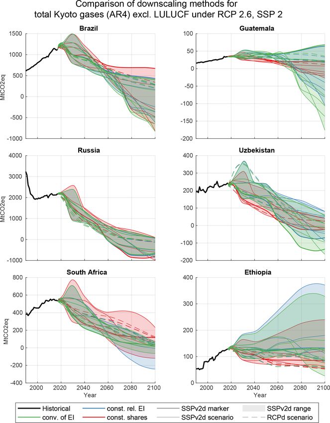
1012                                            J. Gütschow et al.: Country pathways based on the RCP and SSP scenarios

   We have investigated several different options to circum-       narios define the maximal forcing level for each SSP, while
vent this problem including dynamical downscaling algo-            the minimal level was found implicitly because the forcing
rithms, which downscale data year by year and can use al-          level of low RCPs could not be attained for all SSPs.
ternate algorithms when regional emission intensity is near
zero. However, fine tuning the parameters to deal with the         3.1.1   SSPv2 IAM runs (SSPv2d)
transition to negative emissions for several scenarios proved
to be very complicated, while the results were often very sim-     During the integrated assessment model (IAM) implementa-
ilar to the very simple solution of moving the convergence         tions of RCP–SSP combinations (SSPv2) it was found that
year to before the transition to negative emissions. After that    some combinations can not be implemented. Figure 8 in Ri-
year all countries follow the same emission intensity path-        ahi et al. (2017) illustrates the carbon prices needed to reach
way. The steep reduction in emissions and emission inten-          a certain mitigation level under a given SSP. The figure also
sity does not leave much freedom for the downscaling (see          shows that the RCP8.5 forcing is only reached for SSP5. All
also Fig. 1). All countries have to rapidly reduce emissions       other SSPs have baseline emissions leading to a lower cli-
to meet the prescribed regional pathway. Furthermore, as de-       mate forcing. For SSP1, RCP6 is the baseline; for SSP2–
scribed in Sect. 2.3.1 there are conceptual problems with          4, the baseline forcings are between RCP6 and RCP8.5.
convergence years set to later than the transition to nega-        Under SSP3, the low-emission scenario of RCP2.6 can not
tive emissions. We therefore use the simple but transparent        be attained, and under SSP5 one model was unable to at-
approach of early convergence. The calculation itself is not       tain sufficiently low emissions. The IAM implementations of
changed, but yc is adjusted to be the last year before the tran-   SSP scenarios use an additional intermediate forcing level
sition to negative emissions. This is done on a per gas level.     of 3.4 W m−2 (Riahi et al., 2017), which can be reached un-
Only CO2 pathways have negative emissions; consequently            der all SSP storylines. Additionally, SSPv2 contains a new
only yc of CO2 is adjusted. The downside of this approach          strong mitigation pathway reaching a forcing level of only
is that it impacts the assumptions of convergence and elim-        1.9 W m−2 (Rogelj et al., 2018). This forcing level is attained
inates the possibility to define different convergence speeds      for SSP1, 2, and 5. Only a single model could attain a forcing
for different socio-economical storylines. Figure 2 gives an       of 1.9 W m−2 under SSP4, and no model could under SSP3
overview of the steps of the downscaling process.                  (see Rogelj et al., 2018, Fig. 5).
                                                                      We downscale all SSPv2 runs, both marker and other.
3     Input data and preprocessing                                 An overview is shown in Table 1. However, not all sce-
                                                                   narios have been implemented by all modeling groups (see
This section provides an overview of the input data. It covers     Appendix B1). For each SSP a different IAM provided the
the RCP and SSP scenarios (Sect. 3.1) and their implementa-        respective illustrative marker scenario. Namely those were
tion including the choice of scenarios for international ship-     for SSP1: IMAGE (Integrated Model to Assess the Global
ping and aviation (Sect. 3.1.3), the region definitions used in    Environment; van Vuuren et al., 2017), SSP2: MESSAGE
the models (Sect. 3.3), the countries covered by the datasets      (Model for Energy Supply Strategy Alternatives and their
(Sect. 3.3), and the covered sectors and gases (Sect. 3.4). Fur-   General Environmental Impact; Fricko et al., 2017), SSP3:
thermore, the historical data used to downscale the RCP and        AIM/CGE (Asia-Pacific Integrated Model/Computable Gen-
SSP scenarios are introduced in Sect. 3.2.                         eral Equilibrium; Fujimori et al., 2017), SSP4: GCAM4
                                                                   (Global Change Analysis Model; Calvin et al., 2017), and
                                                                   SSP5: REMIND–MAgPIE (Regional Model of Investment
3.1    Scenario description
                                                                   and Development; Model of Agricultural Production and its
Two datasets are produced based on two sets of scenar-             Impacts on the Environment; Kriegler et al., 2017).
ios: RCPd, based on the RCP scenarios (van Vuuren et al.,
2011a), which are downscaled using the SSP basic elements,         3.1.2   RCP and SSP basic elements (RCPd)
and SSPv2d, based on the SSPv2 IAM implementations
of the SSP scenarios, which come with consistent socio-            To select sensible combinations of RCP scenarios and SSP-
economic data that are used for downscaling (Riahi et al.,         basic-elements scenarios we use the SSPv2 IAM runs as a
2017; Rogelj et al., 2018).                                        basis. The combination of RCP8.5 with SSP1 is excluded be-
   Not all combinations of RCP GHG forcing scenarios and           cause no model reached emissions significantly above RCP6
SSP storylines are meaningful, as some SSP storylines im-          levels, and the SSP1 storyline of a rapid sustainable de-
ply, e.g., emissions that lead to forcing levels below RCP8.5,     velopment is not compatible with RCP8.5 emission levels.
while other SSPs imply high unmitigated emissions, for             The baseline forcings of SSP2–4 do not reach 8.5 W m−2 ;
which it is unrealistic to be mitigated to the lowest RCP forc-    however, forcings are significantly above 6 W m−2 for SSP2
ing levels without substantially changing the socio-economic       (6.5–7.3 W m−2 ) and SSP3 (6.7–8.0 W m−2 ) (Riahi et al.,
storyline. For the SSPv2 scenarios the possible combinations       2017). Thus we include the combination of RCP8.5 with
were determined by the IAMs: the SSP-specific baseline sce-        SSP2 and 3. SSP4 models a very unequal socio-economic de-

Earth Syst. Sci. Data, 13, 1005–1040, 2021                                         https://doi.org/10.5194/essd-13-1005-2021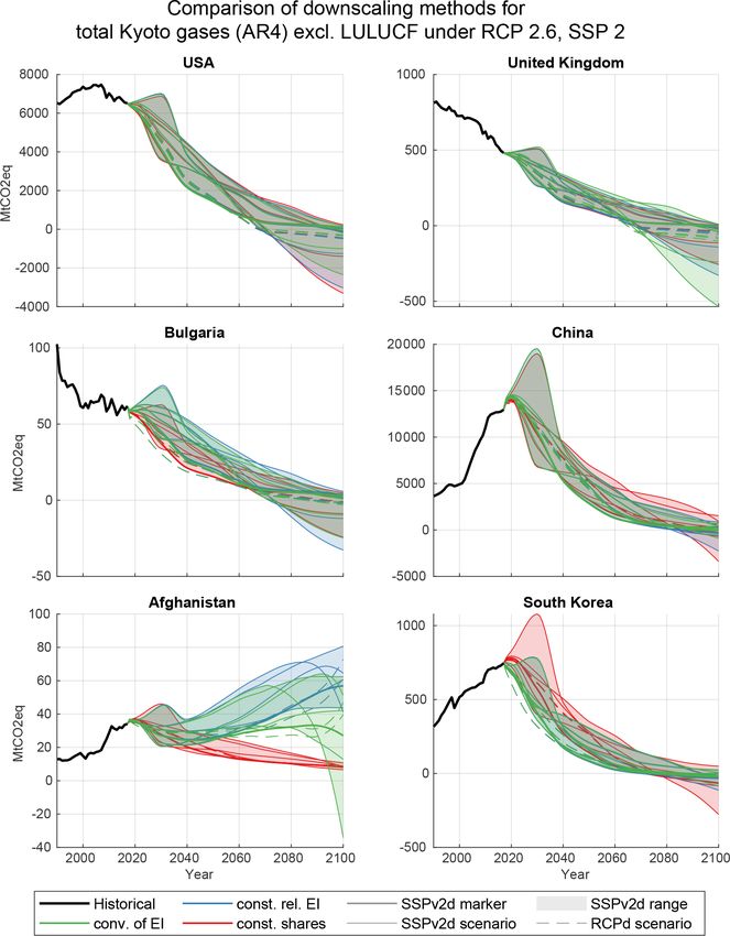
J. Gütschow et al.: Country pathways based on the RCP and SSP scenarios 1013
Table 1. Forcing levels attained by SSPv2 studies. See Riahi et al. (2017), Calvin et al. (2017), and Rogelj et al. (2018). For SSP1, RCP6 is
the baseline forcing for all models except WITCH (World Induced Technical Change Hybrid), which has a slightly higher baseline (BL) such
that RCP6 is a mitigation scenario. “x” means that the forcing level could be attained by all models that implemented it, and “(x)” means that
it could be attained by at least one model but not in the marker implementation. All forcings in W m−2 .
SSP1 SSP2 SSP3 SSP4 SSP5
Baseline 5.8 6.5–7.3 6.7–8.0 6.4 8.5
RCP8.5 x = BL
RCP6 (x) = BL x x x x
RCP4.5 x x x x x
3.4 W m−2 x x x x x
RCP2.6 x x x (x)
1.9 W m−2 x x (x) x
Marker IMAGE MESSAGE AIM/CGE GCAM4 REMIND
Table 2. Combination of RCP scenarios with SSP-basic-elements from aviation and shipping likely differ from growth
country results considered in this study. rates of general fossil CO2 emissions, the inclusion
changes the growth rates of the regional emission path-
SSP1 SSP2 SSP3 SSP4 SSP5 ways. As there are no readily available consistent CO2
RCP8.5 x x x pathways for international shipping and aviation for the
RCP6 x x x x x original RCP scenarios, they have to be either generated
RCP4.5 x x x x x or taken from other scenarios. The RCPs provide data
RCP2.6 x x x x for several gases and pollutants for aviation and ship-
ping. One approach is to try to calculate CO2 emissions
consistent with the RCP emissions from other gases us-
velopment with low reference emissions, as only a small part ing correlations between CO2 and the other gases ob-
of the world has high consumption levels, and cheap mitiga- tained from scenarios which cover all gases. However,
tion options, as investment in new technologies is high. The using the shipping and aviation time series from Owen
baseline forcing of 6.4 W m−2 (Calvin et al., 2017) is above et al. (2010) and QUANTIFY (2010) to compute the
RCP6 but significantly below RCP8.5. We thus exclude the correlations, no consistent CO2 pathways could be gen-
combination of SSP4 with RCP8.5. erated, as results based on different gases were not con-
In the IAM studies it was also found that the SSP3 story- sistent. We therefore have to use external scenarios. We
line does not allow for sufficient mitigation to reach RCP2.6 use the CMIP6 emission scenarios from Gidden et al.
forcing levels (Riahi et al., 2017). Consequently, we exclude (2019), which are based on the RCP forcing and SSP
this combination. The combination of SSP5 with RCP2.6 is storylines and are consistent with the RCPs on the basis
included, as most models used for SSPv2 can attain the nec- of RCP forcing targets but not the pathways to reach
essary forcing levels. All combinations considered are shown these targets. See Table 3 for our choice of CMIP6
in Table 2. bunker scenarios for the RCPs.
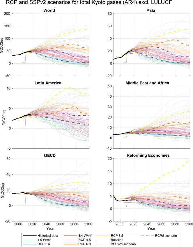
Figure 3 gives an overview of the RCP and SSPv2 scenar- The CMIP6 scenarios contain emissions for interna-
ios. Figures for individual gases are available in Sect. S2.1 in tional shipping for CO2 and CH4 as well as aviation
the Supplement. emissions for CO2 . Unfortunately N2 O emissions are
only given as a national total. We thus compute a factor
3.1.3 Emissions from international shipping and aviation of N2 O over CO2 from historical data (2007–2012 av-
erage from Smith et al., 2014) and construct scenarios
Emissions from international shipping and aviation (bunker from the CO2 scenarios, assuming this factor is constant
fuels) are not attributed to individual countries under the over time. As N2 O emissions only contribute roughly
UNFCCC. Therefore they need special consideration in the 1 % of total bunker emissions this simplification has
downscaling process. very limited impact. To downscale total aviation emis-
sions to domestic and international aviation, we use the
– RCPd. Emissions from international shipping and avi- shares from the historical CMIP6 emission data (Hoesly
ation are included in the RCP scenario emissions. For et al., 2018).
CO2 and N2 O (marine only) however, they are not pro-
vided as individual emission time series but included – SSPv2d. The SSPv2 scenarios as presented in the
in the regional emissions. As growth rates of emissions SSPDB (International Institute for Applied Systems
https://doi.org/10.5194/essd-13-1005-2021 Earth Syst. Sci. Data, 13, 1005–1040, 2021
1014 J. Gütschow et al.: Country pathways based on the RCP and SSP scenarios
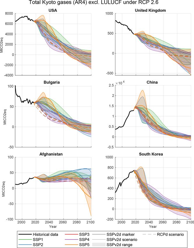
Figure 3. RCP and SSPv2 scenarios for total Kyoto GHG emissions (AR4 GWPs; global warming potentials) excluding LULUCF (land use,
land use change, and forestry). Scenarios are not harmonized to historical data. Historical data shown are from PRIMAP-hist with bunker fuel
CO2 emissions added from CDIAC (Carbon Dioxide Information Analysis Center) data (Boden et al., 2017; Andres et al., 1999; Marland
and Rotty, 1984).
Analysis SSP scenario database; IIASA, 2018; Ri- the same as for the RCP scenarios with a few small ad-
ahi et al., 2017) do not include explicit bunker emis- justments. External scenarios are needed for all gases
sions. As for the RCPs we use the CMIP6 scenarios, including CH4 , which has explicit data in the RCP sce-
which also offer implementations of the new 1.9 and narios but not in SSPv2. For the SSP baseline scenar-
3.4 W m−2 forcing targets. We base the bunker emis- ios we use the SSP3 baseline implementation reach-
sions on the forcing targets only and use the same emis- ing 7.0 W m−2 for all SSPs. The choice of scenarios is
sion time series for all SSPs. The methods are generally shown in Table 3.
Earth Syst. Sci. Data, 13, 1005–1040, 2021 https://doi.org/10.5194/essd-13-1005-2021J. Gütschow et al.: Country pathways based on the RCP and SSP scenarios 1015
Table 3. Choice of SSP–CMIP6 bunker pathways to complement data for both emissions and socio-economic variables. We
the RCPs and SSPv2 scenarios with CO2 , N2 O, and CH4 emissions. do not use the historical data provided with the RCP and
CH4 is only needed for the SSPv2 scenarios, as data are available SSP scenarios, as we want to use latest historical compila-
for the RCPs. Baseline emissions are between RCP6 and RCP8.5 tion datasets (Gütschow et al., 2019, 2016).
for most SSPs. GLOBIOM: GLObal BIOsphere Model.
RCP Aviation and shipping scenario 3.2.1 Historical emission data
Baseline SSP3 7.0 BL AIM/CGE We use the PRIMAP-hist (v2.1) historical emission time se-
RCP8.5 SSP5 8.5 BL REMIND–MAgPIE ries (Gütschow et al., 2016, 2019). It combines multiple data
RCP6 SSP4 6.0 GCAM4 sources into one comprehensive dataset covering all Kyoto
RCP4.5 SSP2 4.5 MESSAGE–GLOBIOM GHGs, all sectors, all countries, and all years from 1850 to
3.4 W m−2 SSP4 3.4 GCAM4 2017. Emission data for some gases and sectors are inter-
RCP2.6 SSP1 2.6 IMAGE polated for the last years. The highest priority during the
1.9 W m−2 SSP1 1.9 IMAGE combination of time series from different sources is given to
data which have been reported to the UNFCCC by countries.
The dataset can be viewed on Paris Reality Check (PRIMAP,
In the scenarios from two of the models (IMAGE and 2020) and is openly accessible (Gütschow et al., 2019).
AIM/CGE) there is a slight (< 1 GtCO2 eq.) discrep-
ancy between global emissions and the sum of the re-
gional emissions. The discrepancy is decreasing in time 3.2.2 Historical socio-economic data
towards 2100. International bunkers are a good explana- We use the PRIMAP-hist historical socio-economic time se-
tion for additional global emissions. However, the dis- ries (Gütschow, 2019). It is constructed using the same meth-
crepancies are much smaller than any bunker estimate, ods as the PRIMAP-hist emission time series.
especially in the future. We thus discard the global data For population data we use the UN population prospects
and work with the regional data as for all other scenar- (UN DESA/Population Division, 2019) and fill gaps and
ios. missing countries from the database of the World Bank’s
The bunker scenarios are shown in Fig. 4. World Development Indicators (WDIs) (The World Bank,
To create scenarios excluding bunker emissions, we sub- 2019b, a). HYDE 3.2 (History Database of the Global En-
tract the bunker emissions from the regional pathways using vironment) data are used for extrapolation into the past until
the historical CO2 bunker emissions from CDIAC (Boden 1850 (Klein Goldewijk et al., 2017; Klein Goldewijk, 2017).
et al., 2017; Andres et al., 1999; Marland and Rotty, 1984) GDP data are based on purchasing-power-parity-adjusted
(2004–2014 average) to downscale the global aviation and (PPP-adjusted) data from the Penn World Table (Feenstra
shipping pathway to the region level. This does not take into et al., 2015, 2019). Missing data are filled using the 2018
account the development of regional emissions and regional Maddison Project database (Bolt et al., 2018b, a) and WDIs.
economies, but as it is unclear how the international bunker Finally we fill missing historical data from a processed
emissions were calculated and assigned to regions when cre- version of the older Maddison Project data (Geiger, 2018;
ating the RCP data, a more sophisticated method would not Geiger and Frieler, 2017; Bolt and van Zanden, 2014; Mad-
necessarily lead to better results. dison Project, 2013; see also Gütschow, 2019). The choice
Bunker emissions also depend on the socio-economic sto- of PPP-adjusted GDP has two reasons: firstly, for compat-
ryline, not only the emission scenario, so selecting the bunker ibility reasons, as the SSP data are given in PPP-corrected
pathways solely based on the RCP forcing levels and not form, and, secondly, PPP-adjusted GDP is more comparable
based on the SSP storylines, which govern, e.g., trade pat- between countries than market-exchange-rate-based (MER-
terns, is a simplification. There are two reasons for this: based) GDP, which is important for the downscaling process
firstly, for gases that are not well mixing (i.e., all except CO2 as the process assumes convergence of emission intensities.
and N2 O, but of these we only use CH4 here) bunker data
are already given for the RCPs, and, secondly, there are no 3.3 Regions and country coverage
bunker scenarios available for all different RCP–SSP combi-
nations, so basing the selection of bunker scenarios on both Here, we provide information on the regions used for the
RCP and SSP would require several assumptions. input data and the conditions under which countries are in-
cluded in the input data and the final dataset. For a country
to be available in the final time series it needs to be included
3.2 Historical data
in the SSP-basic-elements GDP time series and the historical
Our aim is to create a set of scenarios that is directly us- data for both emissions and GDP, and for the SSPv2 scenar-
able for climate policy research and analysis. It is important ios it further needs to be included in the region definitions of
that the country-specific pathways are in line with historical the IAMs. Table S2 of the Supplement gives an overview of
https://doi.org/10.5194/essd-13-1005-2021 Earth Syst. Sci. Data, 13, 1005–1040, 20211016 J. Gütschow et al.: Country pathways based on the RCP and SSP scenarios
Figure 4. Scenarios for bunker fuels used to remove bunker emissions from the RCP and SSPv2 emission scenarios. Aviation emissions are
only available for CO2 . Historical data are from CMIP6 (Hoesly et al., 2018) for CO2 and CH4 . For N2 O we use data from the Interna-
tional Maritime Organization (IMO) and EDGAR v4.3.2 data (Emissions Database for Global Atmospheric Research; JRC and PBL, 2017;
Janssens-Maenhout et al., 2019) for the time not covered by the IMO data.
available countries in each scenario, the input data, and the Each of these regions is downscaled individually and not
final dataset. influenced by values from other regions. Where countries
are missing in the socio-economic pathways or the historical
3.3.1 RCPd emission data, they are ignored, and the regional emissions
are split among the available countries. The SSP basic ele-
The emission pathways provided with the RCP scenarios di- ments do not cover all countries but, depending on the mod-
vide the world into five regions (IIASA, 2009): eling group, leave out some smaller countries. This excludes
several small states such as most of the small island states.
– ASIA: Asian countries
Those states are therefore excluded from the downscaled
– LAM: Latin America dataset. A list of those countries can be found in Sect. S1.3.7
in the Supplement. Some countries do not have data for all
– MAF: Middle East and Africa variables and are included in the final datasets with the avail-
able variables.
– OECD90: OECD (Organisation for Economic Co-
The socio-economic scenarios provided by the SSPbe
operation and Development) countries as of 1990 and
modeling groups contain population (KC and Lutz, 2017)
some Pacific island states
and GDP (Dellink et al., 2017; Leimbach et al., 2017; Cre-
– REF: reforming economies (former Soviet Union). spo Cuaresma, 2017) projections on a per country or de-
tailed per region level. Population data are only provided
Earth Syst. Sci. Data, 13, 1005–1040, 2021 https://doi.org/10.5194/essd-13-1005-2021J. Gütschow et al.: Country pathways based on the RCP and SSP scenarios 1017
by the IIASA (International Institute for Applied Systems 3.4.1 RCPd
Analysis) group; the other groups (OECD and PIK) use the
The RCPs include information for the Kyoto GHGs (CO2 ,
IIASA population projections to build their GDP projections.
CH4 , N2 O, and the fluorinated gases (F-gases)) as well as
GDP data are provided in purchasing-power-parity-corrected
several other substances (CO, SO2 , NH3 , NOx , black car-
(PPP-corrected) form in 2005 international dollars (Geary–
bon (BC), organic carbon (OC), volatile organic compounds
Khamis dollar; GKD)1 . The PIK data are provided on a
(VOCs), and ozone-depleting substances (ODSs)). Here we
level of 32 world regions. We downscale it to the individual-
focus on the Kyoto GHGs because of their special relevance
country level using the underlying IIASA population data
to the UNFCCC negotiations and availability of historical
and the method introduced in Sect. 4.2. In Sect. S1.2 in the
data. Additional substances can be added if there is demand
Supplement we present the exact region definitions and list
from the scientific community and where historical data are
of missing countries for each modeling group.
available (for historical data see Hoesly et al., 2018; Mein-
shausen et al., 2017). Fluorinated gases are treated as one gas
3.3.2 SSPv2d at the moment. Historical data for fluorinated gases are avail-
able at a level of aggregate HFCs (hydrofluorocarbons), ag-
The SSPv2 IAM implementations provide both emission and gregate PFCs ((per-)fluorocarbons), and SF6 for all countries,
socio-economic data on the level of five world regions sim- but to be consistent with the SSPv2 scenarios which only pro-
ilar to the regions used in the RCPs. However, the exact re- vide aggregate data for fluorinated gases, we do not use this
gion definitions in terms of included countries differ from more detailed data in the downscaling process. Some sub-
model to model. A detailed list with region definitions is stances such as black carbon need other downscaling meth-
available from the SSP database (IIASA, 2016). We use the ods, as they are often co-emitted with gases like CO2 . This
model-dependent region definitions to downscale both socio- correlation of emissions has to be taken into account in the
economic and emission data. GDP data are provided in PPP- downscaling.
corrected form in 2005 dollars (GKD and USD). The socio- The sectoral detail of the emission data provided with the
economic data of the SSPv2 runs is based on the IIASA RCPs differs between the greenhouse gases. The data for the
country population data (KC and Lutz, 2017) and the OECD most important gas, CO2 , are only resolved into emissions
GDP data (Dellink et al., 2017). Consequently, we use these from land use, land use change, and forestry (LULUCF)
datasets to downscale the IAM data to the country level using and emissions from fossil fuels and industry. We employ the
an external-input-based downscaling method (see Sect. 4.3). same sectoral resolution for the other Kyoto GHGs. N2 O data
In Sect. S1.3 in the Supplement we present a list of missing are only available as a national total. As LULUCF emissions
countries for each model. only constitute a fraction of roughly 3 % of global N2 O emis-
sions (in 2015, see Gütschow et al., 2018), we use the total
emissions as a proxy for fossil fuel and industrial emissions.
3.4 Sectors and gases
The sector and gas resolution of the historical time series is 3.4.2 SSPv2d
finer than the resolution of the scenarios for all sectors, gases,
In principle the SSPv2 scenarios cover the same substances
and countries. Thus, the resolution of the final dataset is de-
as the RCP scenarios. However, fluorinated gases are only
termined by the resolution of the scenario data. In this section
available as a global-warming-potential-weighted aggregate
we are only considering emission time series, as population
time series. Therefore, fluorinated gases (F-gases) are treated
and GDP are given as national totals.
as one substance. While the global warming potential (GWP)
LULUCF emissions are subject to high annual fluctua-
used for the F-gas basket is not explicitly given, the data are
tions, and their development very much depends on indi-
consistent with a Kyoto GHG basket2 created using GWPs
vidual countries’ policies. Furthermore, the scenario data of-
from the IPCC’s “Fourth Assessment Report” (AR4). There-
ten have positive emissions for regions for which historical
fore, we assume that the F-gas basket has been calculated
data show negative emissions in the past years. In this case
based on AR4 GWPs.
the past (negative) emission shares and emission intensity
In terms of sectors the SSPv2 scenarios offer less detail
are no indicator for projected (positive) emissions. LULUCF
than the RCPs: CO2 , CH4 , and N2 O emissions are available
downscaling thus needs several strong assumptions which we
for the national total and a sector called “land use” indepen-
think users of the data should make knowingly instead of un-
dently. For CO2 and for some scenarios also for CH4 , addi-
knowingly using our assumptions. In conclusion we exclude
tional time series for emissions from fossil fuels and industry
LULUCF data from the downscaling as done in van Vuuren
are provided. However, the employed definition of the land
et al. (2006, 2007).
use sector differs from the definition in the IPCC categoriza-
1 Actually, data are provided in 2005 US dollars (USD), but for 2 The Kyoto GHG basket is the GWP-weighted sum of CO ,
2
a PPP-corrected GDP this equals 2005 international dollars (GKD). CH4 , N2 O, and the fluorinated gases (HFCs, PFCs, and SF6 ).
https://doi.org/10.5194/essd-13-1005-2021 Earth Syst. Sci. Data, 13, 1005–1040, 20211018 J. Gütschow et al.: Country pathways based on the RCP and SSP scenarios
tions. The high emission levels for CH4 and N2 O suggest 4.1 Preparation of RCP and SSP data
that, rather than for land use only, the time series cover emis-
RCP and SSP data have to be preprocessed such that data
sions from the agriculture, forestry, and land use (AFOLU)
are available for all sectors, gases, and years needed for the
sector. For CO2 this is not a practical problem, as agricultural
downscaling.
CO2 emissions contribute less than 0.1 % to total CO2 emis-
sions (Gütschow et al., 2019), and we use the land use sector
as a proxy for LULUCF. However, for N2 O and CH4 this is 4.1.1 RCP data
not possible, as agricultural contributions are substantial. We
The RCP data only offer values every 10 years. It is inter-
thus use national total emissions as a proxy for fossil fuel and
polated using MATLAB’s “pchip” function to obtain yearly
industrial emissions, as LULUCF emissions for these gases
values needed for harmonization. The data do not resolve
account for only 3 % (N2 O) and 4 % (CH4 ) of national total
any categories for N2 O and fluorinated gases. National to-
emissions (Gütschow et al., 2018). Emissions of fluorinated
tal values are copied to obtain values for emissions exclud-
gases are available as a national total only, which suffices, as
ing land use for fluorinated gases and N2 O. For methane
they originate from industrial sources only.
higher-level categories are aggregated from the lower-level
categories available in the RCP data. We build the HFC, PFC,
4 Downscaling of RCP and SSPv2 scenarios aggregate F-gas, and Kyoto GHG baskets for GWPs from the
IPCC’s “Second Assessment Report” (SAR) and “Fourth As-
The following describes the generation of the downscaled sessment Report” (AR4)
RCP and downscaled SSPv2 scenarios step by step from the Time series excluding bunker emissions are created in ac-
preparation of input data to the combination of historical and cordance with Sect. 3.1.3.
scenario data for the final time series.
– Data preparation. The RCP and SSP data are processed 4.1.2 SSP basic elements
as described in Sect. 4.1. Historical data do not need The SSP-basic-elements country-level data are first summed
preprocessing at this step. to the country definitions used for the historical GDP and
population data. GDP data are given in PPP-corrected 2005
– Downscaling of socio-economic data. Not all socio- US dollars (USD) and have to be converted to 2011 inter-
economic data have country resolution. The PIK GDP national dollars (GKD) (see Appendix C1 for details). As
data need downscaling to the country level (Sect. 4.2), IIASA and OECD data cover a slightly different set of coun-
and the SSPv2 socio-economic data need it as well tries, we create a composite GDP source which uses the
(Sect. 4.3). After the downscaling, all socio-economic OECD GDP data as the basis and fills missing countries from
data are processed to match the country definitions of the IIASA data. See Table 2 of the Supplement for details.
the historical emission data.
– Generation of socio-economic scenarios. In this step 4.1.3 SSPv2 socio-economic data
GDP and population time series from all SSP scenar-
The SSPv2 socio-economic scenarios are interpolated to ob-
ios are combined with historical data (Sect. 4.4). The
tain yearly values from time series with a temporal resolution
socio-economic part of the dataset is finalized with this
of 10 years. No further processing is done at this point.
step and is used as input for the emission downscaling.
– Downscaling of RCP and SSPv2 emission data. RCP 4.1.4 SSPv2 emission data
data are downscaled using the SSP-basic-elements
The SSPv2 emission data are interpolated to obtain yearly
country data (Sect. 4.5), while SSPv2 data are down-
values. N2 O and CH4 emissions excluding LULUCF are ob-
scaled using the downscaled SSPv2 socio-economic
tained from national total emissions. Existing time series
data (Sect. 4.3). During the process the downscaling key
are discarded because they do not include agricultural emis-
is harmonized to historical data (Sect. 4.4).
sions. Fluorinated gases are only available as a AR4 GWP-
– Generation of emission scenarios. In the final step the weighted sum. To create a time series for SAR GWPs, re-
downscaled RCP and downscaled SSPv2 emission sce- gional conversion factors from AR4 to SAR are calculated
narios are combined with and harmonized to historical from EDGAR v4.2 data for individual gases using the years
emission data (Sect. 4.6). 2000 to 2012. As for CH4 and N2 O, a copy of national to-
tal F-gas emissions is used for the national total excluding
All operations are carried out independently per scenario, LULUCF. We build Kyoto GHG baskets for SAR and AR4
region and gas. The combination of historical and scenario GWPs.
data is carried out independently per scenario, country, and Time series excluding bunker emissions are created in ac-
gas. cordance with Sect. 3.1.3.
Earth Syst. Sci. Data, 13, 1005–1040, 2021 https://doi.org/10.5194/essd-13-1005-2021You can also read