Using Shapley additive explanations to interpret extreme gradient boosting predictions of grassland degradation in Xilingol, China - GMD
←
→
Page content transcription
If your browser does not render page correctly, please read the page content below
Geosci. Model Dev., 14, 1493–1510, 2021
https://doi.org/10.5194/gmd-14-1493-2021
© Author(s) 2021. This work is distributed under
the Creative Commons Attribution 4.0 License.

Using Shapley additive explanations to interpret extreme gradient
boosting predictions of grassland degradation in Xilingol, China
Batunacun1,2 , Ralf Wieland2 , Tobia Lakes1,3 , and Claas Nendel2,3
1 Department   of Geography, Humboldt-Universität zu Berlin, Unter den Linden 6, 10099 Berlin, Germany
2 Leibniz  Centre for Agricultural Landscape Research (ZALF), Eberswalder Straße 84, 15374 Müncheberg, Germany
3 Integrative Research Institute on Transformations of Human-Environment Systems, Humboldt-Universität zu Berlin,

Friedrichstraße 191, 10099 Berlin, Germany

Correspondence: Batunacun (batunacun@zalf.de)

Received: 25 February 2020 – Discussion started: 9 June 2020
Revised: 27 October 2020 – Accepted: 10 November 2020 – Published: 16 March 2021

Abstract. Machine learning (ML) and data-driven ap-              Land-use change includes various land-use processes, such
proaches are increasingly used in many research areas. Ex-       as urbanisation, land degradation, water body shrinkage, and
treme gradient boosting (XGBoost) is a tree boosting method      surface mining, and has significant effects on ecosystem ser-
that has evolved into a state-of-the-art approach for many       vices and functions (Sohl and Benjamin, 2012). Grassland is
ML challenges. However, it has rarely been used in sim-          the major land-use type on the Mongolian Plateau; its degra-
ulations of land use change so far. Xilingol, a typical re-      dation was first witnessed in the 1960s. About 15 % of the
gion for research on serious grassland degradation and its       total grassland area was characterised as being degraded in
drivers, was selected as a case study to test whether XG-        the 1970s, which rose to 50 % in the mid-1980s (Kwon et
Boost can provide alternative insights that conventional land-   al., 2016). In general, grassland degradation (GD) refers to
use models are unable to generate. A set of 20 drivers was       any biotic disturbance in which grass struggles to grow or
analysed using XGBoost, involving four alternative sam-          can no longer exist due to physical stress (e.g. overgraz-
pling strategies, and SHAP (Shapley additive explanations)       ing, trampling) or changes in growing conditions (e.g. cli-
to interpret the results of the purely data-driven approach.     mate; Akiyama and Kawamura, 2007). In this study, grass-
The results indicated that, with three of the sampling strate-   land degradation is defined as grassland that has been de-
gies (over-balanced, balanced, and imbalanced), XGBoost          stroyed and subsequently classified as some other land use,
achieved similar and robust simulation results. SHAP values      or that has significantly decreased in coverage.
were useful for analysing the complex relationship between          Grassland is a land use that provides extensive ecosystem
the different drivers of grassland degradation. Four drivers     services (Bengtsson et al., 2019). When degraded, the conse-
accounted for 99 % of the grassland degradation dynamics         quences are seen in an immediate decline in these services,
in Xilingol. These four drivers were spatially allocated, and    such as a decrease in carbon storage due to a reduction in
a risk map of further degradation was produced. The limita-      vegetation productivity (Li et al., 2017). About 90 % of car-
tions of using XGBoost to predict future land-use change are     bon in grassland ecosystems is stored in the soil (Nkonya et
discussed.                                                       al., 2016). Furthermore, GD results in a reduction in plant
                                                                 diversity and above-ground biomass available for grazing
                                                                 (Wang et al., 2014). Likewise, GD leads to soil erosion and
                                                                 frequent dusts storms in Inner Mongolia (Hoffmann et al.,
1   Introduction                                                 2008; Reiche, 2014). Drivers of GD are manifold and have
                                                                 been analysed in a range of studies (Li et al., 2012; Liu et
Land-use and land-cover change (LUCC) has received in-           al., 2019; Sun et al., 2017; Xie and Sha, 2012). However,
creasing attention in recent years (Aburas et al., 2019; Diouf   few studies use sophisticated driver analysis to predict spa-
and Lambin, 2001; Lambin et al., 2003; Verburg et al., 2002).

Published by Copernicus Publications on behalf of the European Geosciences Union.
1494                             Batunacun et al.: Using SHAP to interpret XGBoost predictions of grassland degradation

tial patterns of GD (Jacquin et al., 2016; Wang et al., 2018).      land-use change processes, the most prominent of which
A number of studies have addressed the complex relation-            are support vector machines (SVM; Huang et al., 2009,
ship between GD and its drivers (Cao et al., 2013a; Feng et         2010), artificial neural networks (ANN; Ahmadlou et al.,
al., 2011; Fu et al., 2018; Tiscornia et al., 2019a). However,      2016; Yang et al., 2016), classification and regression trees
these studies focus mainly on visualising or describing non-        (Tayyebi and Pijanowski, 2014b), and random forest (RF;
linear relationships between GD and its drivers.                    Freeman et al., 2016). While the different ML approaches
    The aim of developing various land-use models was to ex-        generally perform well in identifying patterns, they remain
plore the causes and outcomes of land-use dynamics; these           a black box and make no contribution to our understand-
models were implemented in combination with scenario                ing of how the underlying drivers act on the LUCC process.
analysis to support land management and decision-making             Compared to linear methods such as logistic regression, ML
(National Research Council, 2014; Ren et al., 2019). Most           models often achieve higher accuracy and capture non-linear
such models are statistical models, such as logistic regres-        land-use change processes. Likewise, ML models relax some
sion models or models based on principle component analy-           of the rigorous assumptions inherent in conventional models,
sis (Li et al., 2013; Lin et al., 2014) or Bayesian belief net-     but at the expense of an unknown contribution of parameters
works (Krüger and Lakes, 2015). Some such models are spa-           to the outcomes (Lakes et al., 2009). However, the key chal-
tially explicit (e.g. CLUE-S, GeoSOS-FLUS, LTM, Fu et al.,          lenge is to crack the black box and reveal how each driver
2018; Liang et al., 2018a; Pijanowski et al., 2002, 2005; Ver-      affects the land-use change pattern or processes in the ML
burg and Veldkamp, 2004; Zhang et al., 2013); others are            models.
not (e.g. Markov models; Iacono et al., 2015; Yuan et al.,             The extreme gradient boosting (XGBoost) method has re-
2015). Hybrid models, which combine different approaches            cently been developed as a supervised machine learning ap-
to make the best use of the advantages of each model, are           proach (Chen and Guestrin, 2016). XGBoost algorithms have
another important variety. This type of model is used to char-      achieved superior results in many ML challenges; they are
acterise the multiple aspects of LUCC patterns and processes        characterised by being 10 times faster than popular exist-
(Li and Yeh, 2002; Sun and Müller, 2013). Agent-based mod-          ing solutions, and the ability to handle sparse datasets and
els (ABM) simulate land use change decisions based on the           to process hundreds of millions of examples. XGBoost has
behaviour of individual decision-makers. They often con-            already been used in land-use change detection, combined
sider economic and political information to calculate land-         with remote sensing data (Georganos et al., 2018), but has
use change. Cellular automata (CA) models are gridded mod-          not yet been used in the simulation and prediction of land-use
els in which time, space, and state are all discrete. CA mod-       change. Shapley additive explanations (SHAP; Lundberg and
els are spatially explicit and land use change decisions are        Lee, 2017) is a unified approach to explain the output of any
made based on the state of the neighbouring cells (Yang et          ML model and to visualise and describe the complex causal
al., 2014). CA models are often used for the spatial alloca-        relationship between driving forces and the prediction target.
tion of land use and land cover at a high spatial resolution        We propose using SHAP to analyse the driver relationships
(Cao et al., 2019) and may be used in combination with other        hidden in the black box model of XGBoost when employed
models, such as ABM (e.g. Charif et al., 2017; Mustafa et al.,      for land-use change modelling.
2017; Troost et al., 2015; Vermeiren et al., 2016).                    Having earlier used a clustering approach to identify
    In most cases of land-use change, it was either assumed         drivers of GD in a case study in Inner Mongolia (Xilingol
that the relationship between the drivers and the resulting         League; Batunacun et al., 2019), we now use XGBoost and
land-use change is constant over time (Fu et al., 2018; Samie       SHAP to simulate GD dynamics across the same area. We
et al., 2017; Zhan et al., 2007), or the relationships were iden-   are primarily interested in learning whether ML models can
tified as being linear or non-linear but were not interpreted       achieve a better predictive quality than linear methods, in ad-
(Tayyebi and Pijanowski, 2014a). We hypothesise that the            dition to improving our understanding of how grassland de-
relationships between GD and its drivers are mainly non-            grades in Xilingol. With the intention to identify areas with a
linear. We therefore see a need for methods that are capa-          high risk of further degradation and to determine the drivers
ble of analysing and interpreting non-linear relationships be-      responsible for progressive degradation, we used XGBoost
tween GD and dynamic drivers.                                       to generate a data-driven model to explore the GD patterns.
    With the development of computer science, machine learn-        We then used SHAP to open the non-linear relationships of
ing (ML) models have been increasingly used in land-use             the black box model stepwise and transformed these relation-
change modelling (Islam et al., 2018; Krüger and Lakes,             ships into interpretable rules. The resulting model enabled us
2015; Lakes et al., 2009; Tayyebi and Pijanowski, 2014a).           to map the primary GD drivers and GD hot spots in Xilingol.
ML is superior to the human brain when it comes to pattern
recognition in large datasets, e.g. images and sensor fields.
Once the task is defined and the data for training are pro-
vided, ML operates without any further human assistance.
Various ML approaches have been used in the analysis of

Geosci. Model Dev., 14, 1493–1510, 2021                                             https://doi.org/10.5194/gmd-14-1493-2021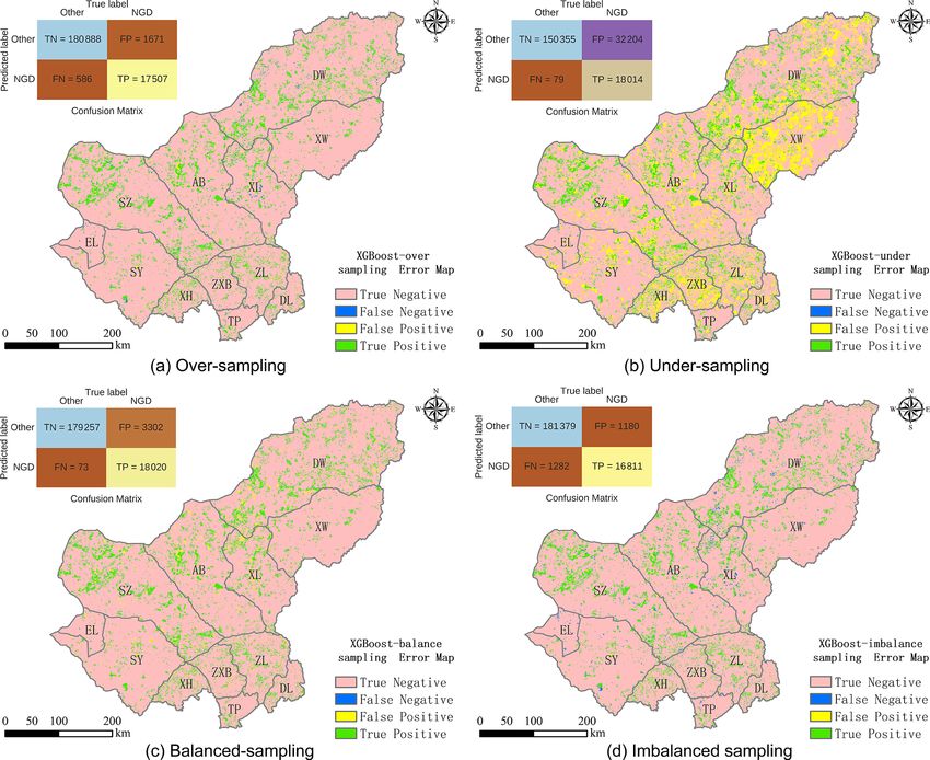
Batunacun et al.: Using SHAP to interpret XGBoost predictions of grassland degradation                                       1495

2     Materials and methods                                         into four categories (see Table 1). All categories were de-
                                                                    scribed as follows: (1) Climate factors, including the an-
2.1    Study area                                                   nual mean temperature (T ) and annual sum of precipita-
                                                                    tion (P ) in the growing season (April to September), were
The Xilingol League is located about 600 km north of Bei-           extracted from the longest available weather dataset (from
jing (He et al., 2004), in the centre of Inner Mongolia. This       1958–2015), in combination with evaluation data and the
administrative unit, covering an area of 206 000 km2 , spans        kriging algorithm, to produce 1 × 1 km2 raster files. (2) Geo-
from 41.4 to 46.6◦ N and from 111.1 to 119.7◦ E (Fig. 1).           graphic factors include elevation (DEM), and slope and as-
The area is dominated by the continental temperate semiarid         pect (extracted from DEM data), which can be treated as
climate. The frequent droughts (in summer) and “dzud” (an           the characteristic of each grid cell. The DEM data were ex-
extremely harsh and snow-rich winter) are the major natu-           tracted from the SRTM 90 m resolution and, after resampling
ral disasters that occasionally lead to catastrophic livestock      using the NEAREST method in ArcGIS, all data were pro-
losses in this region (Allington et al., 2018; Tong et al., 2017;   cessed into 1 × 1 km2 raster files. (3) Distance measures (the
Xu et al., 2014). Xilingol possessed about 18 104 km2 avail-        distance of each pixel centre to urban, rural, road and min-
able pasture resources and 1240.4 × 104 sheep units at the          ing, forest, cropland, dense grass, moderately dense grass,
end of 2015 (Xie and Sha, 2012). Around 1.044 million peo-          sparse grass, and unused land pixels) are widely used fac-
ple lived in Xilingol in 2015, with ethnic Mongolian minori-        tors for different land-use models (Khoury, 2012; Samardžić-
ties accounting for around 31 % and the rural population for        Petrović et al., 2016, 2017; Zhang et al., 2013). All distance
37 % (Batunacun et al., 2019; Shao et al., 2017). Xilingol is a     measures were extracted from LUCC datasets from the years
vast grassland, known for its high-quality meat products, no-       2000 and 2015 using ArcGIS Euclidean distance and pro-
madic culture, rich mineral resources, and ethnic minorities.       cessed into 1 × 1 km2 grids. (4) Socio-economic factors in-
The ongoing degradation of grassland is receiving increasing        clude the gross domestic product (GDP) and population den-
attention. A set of economic stimuli and ecological protec-         sity from 2000 and 2010, and sheep density from 2000 and
tion policies launched in Xilingol were viewed as the root          2015. GDP and population density were obtained from a re-
cause of GD over the past four decades. Although large-scale        sources and environment data cloud platform, CAS (http:
ecological restoration policies were implemented after 2000         //www.resdc.cn/, last access: 8 February 2020); sheep density
in a bid to reduce GD, the problem still persists.                  data were accessed from statistical data, and we converted
                                                                    all livestock data into grassland pixels. Unfortunately, high-
2.2    Grassland degradation
                                                                    resolution GDP and population density data were not avail-
This study defines grassland degradation based on land-use          able for 2015 to match the other data that were recorded for
conversion, involving two kinds of land-use change pro-             that year, so we may assume that GDP and population den-
cesses: (i) the complete destruction of grassland by trans-         sity introduce a bias to the result. While population density
formation to another type of land use (built-up land, crop-         did not change much between 2010 and 2015, GDP changed
land, woodland, water bodies, and unused land), and (ii) a          from CNY 61.4 billion in 2010 to CNY 100.2 billion in 2015
decline in grassland coverage, which includes dense grass           in total over the Xilingol region (GDP data source: http:
deteriorating into moderately dense grass and sparse grass,         //tjj.xlgl.gov.cn/ywlm/tjsj/jdsj/, last access: 1 April 2020).
and moderately dense grass deteriorating into sparse grass          (5) Finally, we identified an area in which we assumed a
(see Fig. S1a in the Supplement). Given that GD is a dy-            strong policy impact in the past and developed a proxy for
namic process, we intended in this study to find the major          the policy effect on grassland degradation. Here, a range of
drivers of newly added grassland degradation (NGD). NGD             ecological protection measures were implemented inside and
refers to the difference in spatial GD extent between two pe-       outside the Hunshandake and Wuzhumuqin sand lands (see
riods. About 13.0 % of the total grassland area (176 410 km2        Fig. S2), e.g. a livestock ban and the promotion of chicken
in 2015) was degraded between 1975 and 2000 (Fig. S1b); a           farming (Su et al., 2015). In a bid to explore policy effects,
further 10.6 % was degraded in 2000–2015 (Fig. S1c). Com-           we assumed that GD is effectively slowed down by various
paring the two periods, approximately 10.2 % of the grass-          policies inside the sandy area (proxy set as 0), while outside
land corresponded to the NGD area across the whole region           the sandy area, land degradation is more likely to happen in
(Fig. S1d). In total 18 279 pixels were extracted from the to-      the absence of any policy effect (proxy set as 1; see Fig. S2).
tal NGD area, while the pixel number of conversion for other
land uses is 181 190 in this study (hereafter: non-NGD).            2.3.1   XGBoost and logistic regression

2.3    Data collection                                              Two algorithms were selected in this study: logistic regres-
                                                                    sion (LR) and XGBoost. LR is a linear method involving
In line with previous studies, a checklist of possible drivers      two parts: the statistic LR and the classification LR. Both
(D) of GD was developed from the literature (Cao et al.,            methods have already been used to simulate land use (Lin
2013b; Sun et al., 2017). A total of 19 drivers were grouped        et al., 2011; Mustafa et al., 2018) and to define the rela-

https://doi.org/10.5194/gmd-14-1493-2021                                              Geosci. Model Dev., 14, 1493–1510, 2021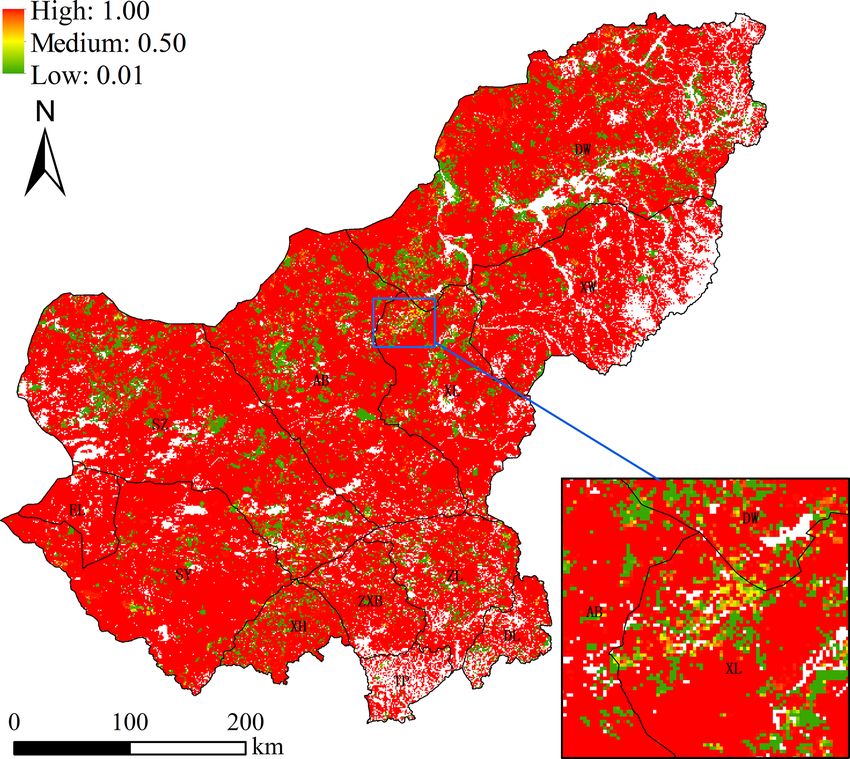
Batunacun et al.: Using SHAP to interpret XGBoost predictions of grassland degradation
https://doi.org/10.5194/gmd-14-1493-2021
Table 1. Definition and derivation of drivers.
Code Name of driver Definition of driver Unit Measures Time series Original format Process approach Data sources
Climate factors
F1 temperature Difference between average temperature/total ◦C Mean temperature 2000, 2015 Grid Kriging via ArcGIS National Meteorological Information
precipitation in growth season (April– and Python language Center (https://data.cma.cn/, last ac-
F2 precipitation September) in Phase 1* and Phase 2* mm cumulative rainfall 2000, 2015 cess: 19 April 2020)
Geographic factors
F3 DEM DEM m – Grid – STRM
F4 slope slope degree – Grid Reclassification http://srtm.csi.cgiar.org/SELECTION/
inputCoord.asp (last access:
1 April 2020)
F5 aspect aspect degree – Grid Reclassification
Distance measures
F6 discrop Change of distance to cropland in 2000 and m Distance 2000, 2015
2015
F7 disforest Change of distance to forest in 2000 and 2015 m Distance 2000, 2015
F8 disunused Change of distance to unused land 2000 and m Distance 2000, 2015
2015
F9 disdense Change of distance to dense grass 2000 and m Distance 2000, 2015
2015
F10 dismode Change of distance to moderate grass in 2000 m Distance 2000, 2015 SHP Euclidean Extraction from land-use data
and 2015
F11 dissparse Change of distance to sparse grass 2000 and m Distance
2015
F12 disurban Change of distance to urban in 2000 and 2015 m Distance 2000, 2015
F13 disrural Change of distance to rural in 2000 and 2015 m Distance 2000, 2015
F14 disroad Change of distance to road in 2000 and 2015 m Distance 2000, 2015
F15 dismine Change of distance to mining in 2000 and 2015 m Distance 2000, 2015
Geosci. Model Dev., 14, 1493–1510, 2021
F16 diswater Change of distance to water in 2000 and 2015 m Distance 2000, 2015
Socio-economic factors
F17 population density Change of population density in 2000 and 2010 Person Person per square kilometre 2000, 2010 Grid Density Resource and Environment data cloud
platform, CAS (http://www.resdc.cn/,
last access: 1 February 2020)
F18 GDP* Change of GDP in 2000 and 2010 Yuan Yuan per square kilometre 2000, 2010 Grid Density
F19 sheep density Change of sheep density in 2000 and 2015 Sheep unit Sheep unit per square kilometre 2000, 2015 Grid Density Statistical data from Xilingol govern-
ment website (http://tjj.xlgl.gov.cn/, last
access: 1 April 2020)
Scenario setting
F20 policy – – (0,1) – Grid – Assumption
* Note: Phase 1 refers to 1975–2000, and Phase 2 refers to 2000–2015. GDP: gross domestic product.
1496
Batunacun et al.: Using SHAP to interpret XGBoost predictions of grassland degradation                                          1497

Figure 1. The location of the Xilingol League in Inner Mongolia and its land uses.

tionship between land-use change and its drivers (Gollnow               of the RF); the n_estimators (controls the number of estima-
and Lakes, 2014; Mondal et al., 2014; Verburg et al., 2002;             tors used for the model); the min_child_weight (controls the
Verburg and Chen, 2000). Here, we use LR as a bench-                    complexity of a model, defines the minimum sum of weights
mark model to compare linear and non-linear methods in                  of all observations required in a child); and lambda (L2
the simulation of land-use change. The optimised parame-                regularisation term on weights). The parameters were opti-
ters of LG are C = 0.1, penalty = l2, solver = “lbfgs”, and             mised using a simple grid search algorithm provided by scikit
multi_class = “multinomial”.                                            (Pedregosa et al., 2011) to estimate the optimal parame-
   Boosting algorithms have been implemented in many past               ters (learning_rate = 0.1, max_depth = 9, n_estimater = 500,
studies, where they often outperformed other ML algorithms              min_child_weight = 3, lambda = 10).
(Ahmadlou et al., 2016; Filippi et al., 2014; Freeman et al.,
2016; Keshtkar et al., 2017; Tayyebi and Pijanowski, 2014a).            2.3.2   Sampling methods
However, traditional boosting algorithms are often subject to
overfitting (Georganos et al., 2018). To overcome this prob-
lem, Chen and Guestrin (2016) presented a new, regularised              Data are often distributed unevenly among different classes
implementation of gradient boosting algorithms, which they              (Vluymans, 2019). Such imbalanced class distribution gen-
called XGBoost (extreme gradient boosting). XGBoost was                 erally induces a bias. Canonical ML algorithms assume that
built as an enhanced version of the gradient boosting deci-             data are roughly balanced in different classes. In real situ-
sion tree algorithm (GBDT), a regression and classification             ations, however, the data are usually skewed, and smaller
technique developed to predict results based on many weak               classes often carry more important information and knowl-
prediction models – the decision tree (DT) (Abdullah et al.,            edge than larger ones (Krawczyk, 2016). It is therefore im-
2019; Freeman et al., 2016). XGBoost provides strong reg-               portant to develop learning from imbalanced data to build
ularisation by adopting a stepwise shrinkage process instead            real-world models (Krawczyk, 2016; Vluymans, 2019). To
of the traditional weighting process provided by GBDT. This             ensure a highly accurate GD model, we introduced four dif-
process limits overfitting, minimises training losses and re-           ferent sampling methods in this study (Fig. S3).
duces classification errors while developing the final model               Balanced sampling. This consists of random data sam-
(Abdullah et al., 2019; Hao Dong et al., 2018).                         pling, resulting in equal-sized samples.
   The XGBClassifier uses the following parameters: learn-                 Imbalanced sampling. This consists of random data sam-
ing_rate (controls learning itself); max_depth (control depth           pling, but with the same share of the sampled class, resulting
                                                                        in unequal sized samples.

https://doi.org/10.5194/gmd-14-1493-2021                                                  Geosci. Model Dev., 14, 1493–1510, 2021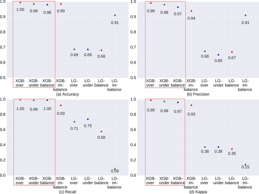
1498                            Batunacun et al.: Using SHAP to interpret XGBoost predictions of grassland degradation

   Over-sampling. Artificial points are added to the minority      ing overall classification accuracy, precision, recall, and the
class of an imbalanced sampling set, making it equal to the        kappa index. Accuracy, precision, and recall were calculated
majority class and resulting in equal sized samples.               based on a confusion matrix (CM) (see Table 2) (He and Gar-
   Under-sampling. Points are removed from a majority class        cia, 2009). For the simulation process, the final model was
of an imbalanced sampling set, making it equal to the minor-       validated using the kappa index, the area under the precision–
ity class and resulting in equal sized samples (He and Garcia,     recall (PR) curve, and recall. The validation indicators are
2009).                                                             defined as follows.
   In the present study, we used these four sampling methods          Overall classification accuracy (ACC) is the correct pre-
to evaluate the model in the context of the sampling method        diction of NGD and other pixels in the whole region. This
and its performance in the training process and the simulation     indicator was used to evaluate the accuracy of the model.
process (see Fig. S3). In our case study, 20 000 pixels (about     Precision is the proportion of correctly predicted positive ex-
10 % of the total; including 18 190 pixels with value 0 indi-      amples (which refers to NGD in this study) in all predicted
cating no-change areas and restored grassland and 1810 pix-        positive examples. Recall is the proportion of correctly pre-
els with value 1 indicating newly added grassland degrada-         dicted positive examples in all observed positive examples
tion) were selected by different sampling methods (Fig. S3)        (the observed NGD) (Sokolova and Lapalme, 2009). In gen-
to train (66 % of the sample size) and test (34 % of the sample    eral, high-precision predictions have a low recall, and vice
size) the model.                                                   versa, depending on the predicted goals. Here, since we focus
                                                                   on NGD and other land-use changes, we use both indicators
2.3.3   SHAP values                                                to evaluate our models.
                                                                      The precision–recall curve provides more information
SHAP (Shapley additive explanations) is a novel approach           about the model’s performance than, for instance, the re-
to improve our understanding of the complexity of predictive       ceiver operator characteristic curve (ROC curve), when ap-
model results and to explore relationships between individual      plied to skewed data (Davis and Goadrich, 2006). The PR
variables for the predicted case (Lundberg and Lee, 2017).         curve shows the trade-off of precision and recall and pro-
SHAP is a useful method to sort the driver’s effects and break     vides a model-wide evaluation. The area under the PR curve
down the prediction into individual feature impacts. Fea-          (AUC-PR) is likewise effective in the classification of model
ture selection is of primary concern when using ML meth-           comparisons. The baseline for the PR curve (y) is determined
ods to process land-use change (Samardžić-Petrović et al.,       by positives (P) and negatives (N). In our study, y = 0.09
2015, 2016, 2017). SHAP values show the extent to which            (y = 18 374/200 652), which means when AUC-PR = 0.09,
a given feature has changed the prediction and allows the          the model is a random model (Brownlee, 2018; Davis and
model builder to decompose any prediction into the sum of          Goadrich, 2006).
the effects of each feature value and explain – in our case –         The kappa index (κ) is a popular indicator used to measure
the predicted NGD probability for each pixel (see Fig. 2). In      the proportion of agreement between observed and simu-
this study, we used SHAP values to sort the driver’s attribu-      lated data, especially to measure the degree of spatial match-
tions, capture the relationship between drivers and NGD, and       ing. When κ > 0.8, strong agreement is yielded between the
map the primary driver for NGD at the pixel level.                 simulation and the observed map, 0.6 < κ < 0.8 describes
   In our study, we define the base value as the value that        high agreement, 0.4 < κ < 0.6 describes moderate agree-
would be predicted by the model if no feature knowledge            ment, and κ < 0.4 represents poor agreement (Landis and
were provided for the current output (mean prediction); we         Koch, 1977).
define the output value as the prediction for this particular         In this study, κ was used to evaluate the agreement and
observation. SHAP values are calculated in log odds. Fea-          disagreement between observed NGD and simulated NGD.
tures that increase the value of the prediction (to the left in    Kappa should be the primary validation measure, followed
Fig. 2) are always shown in red; those that lower the predic-      by AUC-PR (used to evaluate model performance) and recall
tion value are shown in blue (to the right in Fig. 2, Dataman,     (used to evaluate model sensitivity). Features and definitions
2019). In this instance (Fig. 2), disdense (change of distance     of these indicators are given below.
to dense grass) is the primary driver of NGD at this pixel level
(largest value). The fact that the value is positive means that    2.3.5   The structure of the ML model
the risk of NDG increases in line with an increase in distance
to dense grass areas.                                              The ML methodology of simulating GD involves six steps
                                                                   (Fig. S4).
2.3.4   Validation of the model                                     1. Target definition and data collection and processing.
                                                                       The targets of this study are to build a robust ML model
Two validation steps are required for ML models: validation            for simulating NGD, as well as visualising these com-
of the training process and validation of the simulation pro-          plex relationships between various variables and the dy-
cess. For the training process, a robust model was selected us-        namics of GD. A total of 20 drivers of GD were col-

Geosci. Model Dev., 14, 1493–1510, 2021                                            https://doi.org/10.5194/gmd-14-1493-2021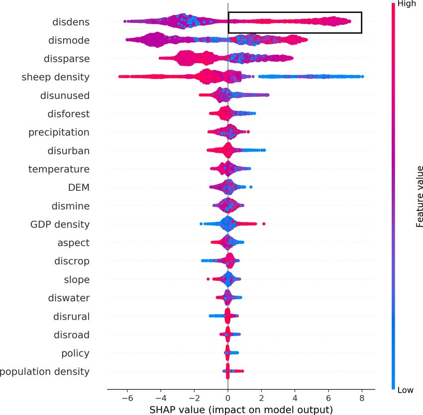
Batunacun et al.: Using SHAP to interpret XGBoost predictions of grassland degradation                                                  1499

Figure 2. Decomposed SHAP values for the individual prediction of an example pixel.

Table 2. Confusion matrix for binary classification of newly added grassland degradation (NGD) and other changes, including four indicators:
false positives (FP), cells that were predicted as non-change but changed in the observed map; false negatives (FN), cells that were predicted
as change but did not change in the observed map for disagreement; true positives (TP), cells that were predicted as change and changed in
the observed map; and true negatives (TN), cells that were predicted as non-change and did not change in the observed map for agreement.

                                                                           Observed values
                                                    Others                  NGD
                    Simulated values
                                          Others    True negatives (TN)     False positives (FP)
                                                                                                   Recall = TP / (TP + FN)
                                          NGD       False negatives (FN)    True positives (TP)
                                                             Precision = TP / (TP + FP)
                                                     ACC = (TP + TN) / (TP + FN + FP + TN)

     lected. All dynamic drivers were processed by GIS into                    5. Model validation and feature ranking. After tuning the
     raster files and exported into ASCII files as final inputs                   model, the most robust model and the driver with most
     for the ML model.                                                            useful information are selected.

  2. Data organisation. The ML model simulates land-use                        6. Explanation. The last step is explaining the model and
     change as a classification task (Samardžić-Petrović et                     the simulation. The model used in the training pro-
     al., 2015, 2017). In the present study, we organise                          cess was published in Zenodo (Batunacun and Wieland,
     this task as a binary classification Y (value 1 and 0,                       2020).
     stand for NGD and Non-NGD); related drivers are x
     (x1 , x2 , x3 . . .. . .xn ), n is the driver identifier, and x de-
     notes the change in value of each driver. The process                 3     Results
     of data standardisation is usually necessary for most
     ML models, but since XGBoost is a tree-based method,                  3.1    Model validation
     it does not require standardisation or normalisation. In
     this case, we performed standardisation only for the lo-              The XGBoost model outperformed the LG model in both
     gistic regression model.                                              training and simulation (Figs. 3 and 4). The LG model seems
                                                                           to be an inappropriate model for understanding NGD in this
  3. Data sampling. This is a necessary step to avoid over-                case. XGBoost yielded robust results in both training and
     fitting or the loss of important information. The sam-                simulation, with indicator values almost entirely above 90 %.
     pling method generally includes balanced and imbal-                      Figure 3 indicates that XGBoost performed very well
     anced sample strategies. In this study, we tested various             across all balanced sampling methods (over-sampling, under-
     balanced sampling strategies to identify the most suit-               sampling, and balanced sampling; red rectangle in Fig. 3) in
     able one.                                                             the training process. Only the imbalanced sampling exhibited
                                                                           a slightly weaker performance in the training process. This
  4. Model building and selection. A ranking was used to                   is mainly due to the balanced sampling datasets, which pro-
     find the best model in each specific case. In our study,              vided more information for the model. In addition, the model
     we defined a model with κ > 0.8 and AUC-PR > 0.09                     was affected less than the imbalanced sampling method by
     as robust, while 0.6 < κ < 0.8 and AUC-PR > 0.09 rep-                 the majority class or unchanged cells (Samardzic-Petrovic et
     resents an acceptable model.                                          al., 2018).

https://doi.org/10.5194/gmd-14-1493-2021                                                       Geosci. Model Dev., 14, 1493–1510, 2021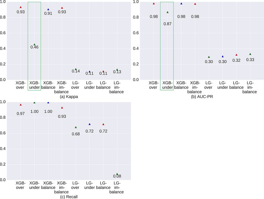
1500                            Batunacun et al.: Using SHAP to interpret XGBoost predictions of grassland degradation

Figure 3. Evaluation of model performance during the training process for newly added grassland between 1975–2015.

   Figures 4 and 5 show the model evaluation results in the          ity of NGD. The gradient colour represents the feature value
simulation process and the spatial prediction maps. XGBoost          from high (red) to low (blue), as previously introduced in
with under-sampling (green rectangle in Fig. 4) yielded the          Fig. 2. As Fig. 6 shows, disdense was the primary driver for
weakest performance compared to the other three sampling             NGD in the study region. The relationship between disdense
methods. This is mainly due to the smaller sample size,              and NGD is non-linear, which can be seen from the SHAP
which prevents the model from extracting sufficient expe-            values being both positive and negative (black rectangle in
rience. As can be seen in Fig. 5b, XGBoost used with the             Fig. 6). The interpretation of the effects of disdense can be
under-sampling method produced the error map with the                summarised as a higher probability of NGD with increasing
highest FP values, where the model predicted non-change              distance from dense grassland (see black rectangle in Fig. 6
points as change points. The under-sampling method is un-            with pink colour on the right).
able to identify NGD points sufficiently well. XGBoost used             Figure 6 shows that driver effects include both linear-
with the over-sampling method caused balanced and imbal-             dominated relationships, such as sheep, GDP, and others, and
anced sampling to have similar and strong prediction abilities       non-linear-dominated relations, such as disdense, dismode,
(see Fig. 4), differing only slightly in their CM indicators         and others. In addition, the figure shows that the most impor-
(see Fig. 5). We finally selected XGBoost combined with the          tant drivers for NGD are the changes of distance to dense,
over-sampling strategy for our study, mainly because of its          moderately dense, and sparse grassland, then followed by
relatively higher values in κ, AUC-PR, and recall (see Fig. 4).      sheep density and the distance to unused land. The effect of
                                                                     policies comes almost at the bottom, indicating that policies
3.2    Driver selection                                              implemented outside sandy areas seem to have little effect
                                                                     on GD. The geographical factors DEM and slope are also
Figure 6 is a summary plot produced from the training                positioned mid-field. The effect of geographical drivers does
dataset; it includes approximately 13 200 points (66 % of the        not appear to be as strong as the effect of other drivers. The
sample size). This plot combines feature importance (drivers         change of distance to mining, located at the bottom for all
are ordered along the y axis) and driver effects (SHAP values        drivers, does not have a strong effect on NGD compared to
on the x axis), which describe the probability of NGD having         other drivers.
occurred. Positive SHAP values refer to a higher probabil-

Geosci. Model Dev., 14, 1493–1510, 2021                                               https://doi.org/10.5194/gmd-14-1493-2021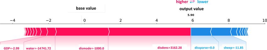
Batunacun et al.: Using SHAP to interpret XGBoost predictions of grassland degradation                                        1501

Figure 4. Evaluation of model performance during the prediction process for newly added grassland between 1975–2015.

   Note that the top rank indicates the most significant ef-         3.3   Relationship between NGD and drivers in the
fects across all predictions. Each point in the cloud to the               XGBoost model
left represents a row from the original dataset. The colour
code denotes high (red) to low (blue) feature values. Positive
SHAP values represent a higher likelihood of NGD, while              SHAP values and spread (Fig. 7) indicate that no linear re-
negative values indicate lower likelihoods. The range across         lationship between driver and prediction could be found for
the SHAP value space indicates the degradation probability,          any of the individual features. Change of distance to dense,
expressed as the logarithm of the odds.                              moderately dense and sparse grass pixels, and change of
   A recursive attribute elimination method was performed to         sheep density were the dominant drivers for NGD. Figure 7a
determine how attribute reduction affects modelling perfor-          indicates that when disdense < 0, the SHAP value is nega-
mance using XGBoost with the oversampling method (see                tive, and when the distance to dense grass areas is small,
Fig. S5; for more details, refer to Samardžić-Petrović et          the likelihood of degradation is also small. The relation-
al., 2015). The results indicate that the first three drivers        ship seems to be more complex for distance to moderately
may already produce a satisfactory model (κ = 0.74, AUC-             dense grass (dismode; Fig. 7b); here, no simple linear inter-
PR = 0.85, recall = 0.92), while adding the fourth driver            pretation is obvious. For distance to sparse grass (dissparse;
can produce a robust model (κ = 0.94, AUC-PR = 0.98, re-             Fig. 7c), the pattern again suggests a rather linear interpre-
call = 0.98). This means that XGBoost used with the over-            tation, which is that the likelihood of degradation increases
sampling strategy can predict NGD with very high accuracy            with decreasing distance. For sheep density, Fig. 7d indicates
using a relatively small amount of data. Figure S6 shows the         that when sheep density decreased, the probability of GD ob-
simulation result using the first four drivers and compares the      viously increased. Policy was not identified as a major driver
results with the observed map.                                       of GD (Fig. 6). However, policy effects obviously have a
                                                                     different impact inside and outside sandy zones. Figure 7e
                                                                     shows that our initial assumption is invalid: the probability
                                                                     of GD increased inside the sandy areas where we assumed
                                                                     effective policy measures to be in place (value 0). This result
                                                                     is also in line with Fig. 7g, which shows that the closer an

https://doi.org/10.5194/gmd-14-1493-2021                                               Geosci. Model Dev., 14, 1493–1510, 2021
1502 Batunacun et al.: Using SHAP to interpret XGBoost predictions of grassland degradation
Figure 5. Error map of different sampling methods using the XGBoost model.
area is to unused land, the more likely it is that degradation the major drivers of NGD, responsible for 9478, 3892, and
will occur there. 1629 NGD pixels, respectively. Sheep density was respon-
We can identify three groups for the remaining 14 drivers. sible for 3042 NGD pixels, ranking third among all drivers.
For GDP and population density (Fig. 7g and h), the likeli- This order differs to that in Figs. 6 and 8 because in those
hood of NGD increases with increasing values. Figure 7i–j cases, ranking is based on the total contribution of all drivers.
indicate that warmer and drier climate conditions increase Figure S7 shows the number of NGD pixels in which a driver
the probability of GD. Figure 7k, l, m, and n indicate that the was dominant or primary. The change of distance to any type
probability of GD rises with closer distances to forest, urban, of grassland was the primary driver for about 82.8 % of the
rural, and water areas. Figure 7o shows a slight SHAP value total NGD pixels; sheep density accounted for 16.8 %. The
pattern, in which the closer to cropland, the more unlikely remaining seven drivers caused less than 1 % of the total
degradation will occur. This is mainly due to transformation NGD. We can see from the spatial pattern that the change
from cropland to grassland. Figure 7p–t do not show any in- of distance to grassland was the major driver for GD in the
terpretable spatial pattern. dense grassland region (counties of DW, XL, and AB), while
in the counties of SZ, SY, ZXB, ZL, and TP, sheep density
3.4 Mapping the primary drivers of NGD was often identified as the major driver.
All drivers’ contributions to NGD were ranked according to 3.5 Regions of high risk for grassland degradation
their SHAP values for each pixel in this study. Figure 8 shows
the primary driver for each NGD pixel. Distance to grass- A probability map of NGD was produced (Fig. 9). Low
land pixels (dense, moderately dense, and sparse grass) were probabilities of NGD were found in the central and north-
Geosci. Model Dev., 14, 1493–1510, 2021 https://doi.org/10.5194/gmd-14-1493-2021Batunacun et al.: Using SHAP to interpret XGBoost predictions of grassland degradation 1503
XGBoost used with the under-sampling method always pro-
duced similar results, irrespective of the size of the dataset
(see Fig. S8). We conclude from this pattern that XGBoost
is also able to use sparse data to reflect real-world problems
(Chen and Guestrin, 2016).
4.2 SHAP values and drivers of grassland degradation
The general idea of introducing SHAP values as a further
tool to analyse XGBoost ranking is to provide a method to
evaluate the ranking with respect to causal relationships. The
original XGBoost ranking is based on the in-built feature se-
lection functions “Gain” (refers to the improvement in accu-
racy provided by a feature), “Weight” (or frequency, refers to
the relative number of a feature occurrence in the trees of a
model), and “Coverage” (refers to the relative numbers of ob-
servations related to this feature). However, these functions
always produce different rankings of drivers (Abu-Rmileh,
2019) due to random components in the algorithms. SHAP
Figure 6. Driver ranking by SHAP values based on the training values introduce two further properties of feature importance
dataset (66 % of sample size) using the over-sampling method. measures: consistency (whenever we change a model such
that it relies more on a feature, the attributed importance
for that feature should not decrease) and accuracy (the sum
ern counties (DW, XL, AB, SZ, ZL ZXB, and XH), while of all feature importance values should equate to the total
high-probability regions were EL, SY, and XW. TP and DL importance of the model; Lundberg, 2018; Lundberg and
in the south were categorised as low-probability regions, due Lee, 2017). Consistency is required to stabilise the ranking
to their lower share of grassland area. throughout the analysis, reducing the change of order in the
ranking to a minimum when the number of identified drivers
changes. The accuracy property of SHAP makes sure that
4 Discussion each driver’s contribution to overall accuracy remains the
same, even when drivers are excluded from analysis. Other
4.1 ML model building and evaluation methods usually compensate for the withdrawal of a driver
from the analysis, which makes the determination of a single
In this study, we defined a general framework for creating an driver’s contribution difficult.
ML model using the XGBoost algorithm for the purpose of The feature ranking based on SHAP values indicated that
analysing and predicting land-use change. XGBoost obtained the change of distance to any type of grassland (dense, mod-
a κ of 93 % and a recall value of > 99 % when used to simu- erately dense, and sparse grass) is the most important driver
late and predict GD in this study. Compared to other popular for any newly added grassland degradation. In this context,
ML learning algorithms, XGBoost exhibited a strong predic- dense and moderately dense grassland areas are more easily
tion ability. In studies where ANN, SVM, RF, CART, multi- degraded than other land-use types, followed by sparse grass.
variate adaptive regression spline (MARS), or LR were used These results are in line with previous studies (Li et al., 2012;
in combination with cellular automata (CA), the recall value Xie and Sha, 2012). Good-quality grassland is more likely to
is usually 54 %–60 % (Shafizadeh-Moghadam et al., 2017). be degraded through increasing human disturbance. An ex-
Ahmadlou et al. (2019) stated that MARS and RF only yield planation for this can be derived from local people’s living
high accuracy in training runs but do not prove to be very strategies. People who live in good-quality grassland areas
accurate in the validating process when simulating land-use are more likely to use grassland for livestock production with
change. higher animal densities, risking overgrazing. Furthermore, Li
Concerning the four sampling strategies we used to test et al. (2012) indicated that good-quality grassland is more
the imbalance issue, we found that all strategies performed likely to be converted to other land-use types, such as crop-
satisfactorily in the training runs. In the simulation, the land. In contrast, people who have lived in sparse grassland
under-sampling strategy yielded a relatively low accuracy regions for centuries have long adapted to low productivity,
(κ = 0.46) model. We assume that removal of data from the reducing their livestock numbers accordingly. They have also
majority class causes the model to lose the important con- developed strategies to cope with variability in weather con-
cepts pertaining to the majority class (He and Garcia, 2009). ditions, e.g. by preparing and storing more fodder and forage.
https://doi.org/10.5194/gmd-14-1493-2021 Geosci. Model Dev., 14, 1493–1510, 20211504 Batunacun et al.: Using SHAP to interpret XGBoost predictions of grassland degradation Figure 7. The SHAP dependence plot for each driver (the y axis is the SHAP value for each driver). Sheep density was identified as the fourth major driver. grass coverage (Nkonya et al., 2016; Wang et al., 2017). However, the SHAP values indicate that when sheep den- However, there is recent evidence that this causal relation- sity decreases, the probability of grassland degradation in- ship has changed. It now appears that farmers increasingly creases. Overgrazing has been the dominant driver for grass- select their livestock numbers according to the carrying ca- land degradation on the Mongolian plateau before, which has pacity of the grazing land (Cao et al., 2013b; Tiscornia et changed the grassland ecosystem significantly towards lower al., 2019b). By passing the “Fencing Grassland and Mov- Geosci. Model Dev., 14, 1493–1510, 2021 https://doi.org/10.5194/gmd-14-1493-2021
Batunacun et al.: Using SHAP to interpret XGBoost predictions of grassland degradation                                          1505

                                                                       play a significant role. For example, in the county of EL, the
                                                                       remaining seven drivers were mainly responsible for NGD.
                                                                       EL has less NGD after 2000 compared with other counties
                                                                       in Xilingol (Fig. S1), and most of the EL area is covered by
                                                                       sparse grass. EL is the most frequented border control point
                                                                       to Mongolia and is subject to intensive tourism.
                                                                          In the sparse grassland and agro-pastoral regions (SZ, SY,
                                                                       ZXB, ZL, and TP), sheep density was identified as the impor-
                                                                       tant driver. This indicates that, even though livestock num-
                                                                       bers have decreased, grassland is still experiencing serious
                                                                       degradation in this region. Here we see additional potential
                                                                       for installing further grassland conservation measures, such
                                                                       as adjusting the livestock number to the grassland carrying
                                                                       capacity.

                                                                       4.3   The current risk of grassland degradation in
                                                                             Xilingol

                                                                       Three regions of different risk classes were identified in the
Figure 8. Spatial patterns of primary drivers for each pixel for       probability map of NGD (Fig. 9). The low-risk region (DW,
NGD.                                                                   XL, AB, SZ, ZL ZXB, and XH) is dominated by good-
                                                                       quality grassland (dense and moderately dense grass). In re-
                                                                       cent decades, this region has suffered from increasing hu-
                                                                       man disturbance, e.g. overgrazing and mining development.
                                                                       However, after 2000, grassland in this region has recovered,
                                                                       mainly as the result of ecological protection projects (Sun et
                                                                       al., 2017). Even though this region is predicted as being less
                                                                       exposed to the risk of land degradation in the future, atten-
                                                                       tion is still required for the restoration process. The high-
                                                                       risk region includes the counties of EL, SY, and XW. EL
                                                                       and SY are covered by a large share of low-quality grass-
                                                                       land, which – due to its own fragility – is likely to be af-
                                                                       fected by extreme climate and human disturbance, more than
                                                                       higher-quality grasslands for example. The recent change in
                                                                       grassland property rights and the establishment of ecological
                                                                       protection projects have also limited the mobility of nomadic
                                                                       herders throughout Xilingol. As a consequence, herders can-
                                                                       not easily change grazing spots if extreme weather occurs;
                                                                       they are then bound to have their cattle graze at the same
                                                                       spots, increasing the pressure on low-quality grasslands in
                                                                       particular (Qian, 2011). For a long time, fragile grassland re-
Figure 9. Degradation probability map for grassland in Xilingol, in-   mained in an equilibrium state with the extreme weather (fre-
cluding a zoom into Xilinhot (XL) for more details. The probability    quent droughts, “dudz”) to which it was exposed, and with
is based on the four most important drivers.                           the nomadic livestock husbandry that the region’s inhabitants
                                                                       practised. However, when the property rights of grassland
                                                                       and livestock were changed from collective to private, the
ing Users” policy (FGMU), the Chinese government issued                nomadic lifestyle was largely abandoned.
a law that regulates livestock numbers based on a previously
calculated carrying capacity. This development has upturned            4.4   The limitations of XGBoost for scenario
the causal relationship between livestock numbers and NGD,                   exploration
reflected by the SHAP value pattern in Fig. 6.
   Besides the four main drivers, seven other drivers also oc-         XGBoost has already scored top in a range of algorithm com-
casionally appear as the main driver for some pixels (Fig. 8).         petitions in the data science community (Kaggle, 2019) due
This highlights the fact that, at the local level, other drivers       to its high accuracy and speed (Chen and Guestrin, 2016).
apart from the four drivers identified as being major can also         ML models extract patterns from data, without considering

https://doi.org/10.5194/gmd-14-1493-2021                                                 Geosci. Model Dev., 14, 1493–1510, 2021
1506 Batunacun et al.: Using SHAP to interpret XGBoost predictions of grassland degradation
any existing expert knowledge, which is why they are in- a typical confusion matrix to evaluate the training process,
creasingly used to identify non-linear relationships (Ahmad- AUC-PR to evaluate the goodness of the ML model, and the
lou et al., 2016; Samardžić-Petrović et al., 2015; Tayyebi kappa index to measure the degree of matching between ob-
and Pijanowski, 2014b). However, ML models require spe- served and simulated values. These validation indicators con-
cific data structures for each problem to which they are ap- sider both the research object and data characteristics. For ex-
plied. In this study, we simulated grassland degradation in ample, when the data size is unbalanced, AUC-PR is a better
two different phases (1975–2000 and 2000–2015). All time choice than AUC-ROC (Brownlee, 2018; Davis and Goad-
series of driver data were organised as model inputs, while rich, 2006; Saito and Rehmsmeier, 2015).
grassland degradation dynamics were organised as predic- SHAP was introduced in this context to provide a causal
tion targets. Although the model achieved high accuracy in explanation of the patterns identified by the ML model. In
predicting NGD in Phase 2, it was not possible to achieve our case, SHAP was used to explain how drivers contribute
acceptable results in simulating both Phase 1 and Phase 2 to grassland degradation processes at the pixel and regional
separately. Second, compared with conventional models, the level, despite their non-linear relationship. According to the
XGBoost model cannot be easily transferred to other regions analysis, the distance to dense, moderately dense, and sparse
for the same research question. Models like CLUE-S and grass and sheep density were the most important drivers that
GeoSOS-FLUS have been widely used in different regions caused new grassland degradation in this region. In addition,
across the world (Fuchs et al., 2018; Liang et al., 2018b; individual SHAP values of sheep density indicated that the
Liu et al., 2017; Verburg et al., 2002). When ML models causal relationship between grassland degradation and live-
are used in other regions, driver data must be collected and stock pressure has changed over time: the increase in sheep
structures adapted. Thirdly, ML models always need to learn density was not the major driver for NGD in Phase 2 of the
sufficiently before they are able to make predictions. This re- land degradation trajectory. Instead, the decrease in the graz-
quires a sufficient amount of data covering historical periods ing capacity of grassland caused a decrease in livestock num-
or different land-use change patterns. bers. The primary driver map of NGD provided a more de-
XGBoost alone is unable to project any scenarios of land- tailed picture of NGD drivers for each pixel, as an impor-
use change based on historical data. However, the method- tant support for grassland management in the Xilingol re-
ology presented here can be applied to quantify alternative gion. The individual SHAP values of each driver may be an
scenarios produced using other approaches, such as conven- important prerequisite for rule-based scenario-building in the
tional, rule-based models (Verburg et al., 2002) or cellular future.
automata (Islam et al., 2018; Shafizadeh-Moghadam et al.,
2017).
Code and data availability. The development of XGBoost and
SHAP values, graphs, and model validation presented in this pa-
5 Conclusion per were conducted using Python. The Python script and re-
lated data used in this study have been archived on Zenodo at
https://doi.org/10.5281/zenodo.3937226 (Batunacun and Wieland,
Machine learning and data-driven approaches are becoming
2020).
more and more important in many research areas. The de- The used XGBoost algorithm including the SHAP library runs
sign and development of a practical land-use model requires well on a modern (Intel or AMD) PC (4 cores or more, 16 GB
both accuracy and predictability to predict future land-use RAM). The training and the simulation were carried out on a Linux
change, a well-fitted model that reflects and monitors the real operating system but should also work on Windows.
world (Ahmadlou et al., 2019). The method framework pre-
sented here for building an ML model and explaining the re-
lationship between drivers and grassland degradation identi- Supplement. The supplement related to this article is available on-
fied XGBoost as a robust data-driven model for this purpose. line at: https://doi.org/10.5194/gmd-14-1493-2021-supplement.
XGBoost showed higher accuracy in training and simula-
tion compared to existing ML models. Combined with over-
sampling, it slightly outperformed in the simulation process. Author contributions. B prepared the paper with contribution from
The simulated map has a high agreement with the observed all co-authors. B gathered and prepared the data, performed the sim-
values (kappa = 93 %). ulations, and analysed the output. RW developed the model code.
We identified six basic steps that should be included in TL and CN developed the research questions and the outline of the
study.
ML model building, and they are also similar for other re-
search applications (Kiyohara et al., 2018; Kontokosta and
Tull, 2017; Subramaniyan et al., 2018). However, different
Competing interests. The authors declare that they have no conflict
validation measures can be introduced in both the training of interest.
process and the simulation process. In this study, we tested
different evaluation measures to evaluate the ML model, e.g.
Geosci. Model Dev., 14, 1493–1510, 2021 https://doi.org/10.5194/gmd-14-1493-2021Batunacun et al.: Using SHAP to interpret XGBoost predictions of grassland degradation 1507
Acknowledgements. The authors express their sincere thanks to the Brownlee, J.: How and When to Use ROC Curves and Precision-
China Scholarship Council (CSC) for funding this research and to Recall Curves for Classification in Python, Mach. Learn.
Elen Schofield for language editing. Mastery, available at: https://machinelearningmastery.com/roc-
curves-and-precision-recall-curves-for-classification-in-python/
(last access: 19 July 2019), 2018.
Financial support. The publication of this article was funded by the Cao, J., Yeh, E. T., Holden, N. M., Qin, Y., and Ren, Z.: The Roles
Open Access Fund of the Leibniz Association. of Overgrazing, Climate Change and Policy As Drivers of Degra-
dation of China’s Grasslands, Nomadic Peoples, 17, 82–101,
https://doi.org/10.3167/np.2013.170207, 2013a.
Review statement. This paper was edited by David Topping and re- Cao, J., Yeh, E. T., Holden, N. M., Qin, Y., and Ren, Z.: The Roles
viewed by two anonymous referees. of Overgrazing, Climate Change and Policy As Drivers of Degra-
dation of China’s Grasslands, Nomadic Peoples, 17, 82–101,
https://doi.org/10.3167/np.2013.170207, 2013b.
Cao, M., Zhu, Y., Quan, J., Zhou, S., Lü, G., Chen, M., and Huang,
References M.: Spatial Sequential Modeling and Predication of Global Land
Use and Land Cover Changes by Integrating a Global Change
Abdullah, A. Y. M., Masrur, A., Adnan, M. S. G., Baky, Md. A. A., Assessment Model and Cellular Automata, Earths Future, 7,
Hassan, Q. K., and Dewan, A.: Spatio-temporal Patterns of Land 1102–1116, https://doi.org/10.1029/2019EF001228, 2019.
Use/Land Cover Change in the Heterogeneous Coastal Region Charif, O., Omrani, H., Abdallah, F., and Pijanowski, B.: A multi-
of Bangladesh between 1990 and 2017, Remote Sens., 11, 790, label cellular automata model for land change simulation, Trans.
https://doi.org/10.3390/rs11070790, 2019. GIS, 21, 1298–1320, https://doi.org/10.1111/tgis.12279, 2017.
Aburas, M. M., Ahamad, M. S. S., and Omar, N. Q.: Spatio- Chen, T. and Guestrin, C.: XGBoost: A Scalable Tree Boosting Sys-
temporal simulation and prediction of land-use change using tem, in Proceedings of the 22nd ACM SIGKDD International
conventional and machine learning models: a review, Environ. Conference on Knowledge Discovery and Data Mining – KDD
Monit. Assess., 191, https://doi.org/10.1007/s10661-019-7330- ’16, pp. 785–794, ACM Press, San Francisco, California, USA,
6, 2019. 2016.
Abu-Rmileh, A.: Be careful when interpreting your fea- Dataman: Explain Your Model with the SHAP Values – Towards
tures importance in XGBoost!, Data Sci., available at: Data Science, Data Sci., available at: https://towardsdatascience.
https://towardsdatascience.com/be-careful-when-interpreting- com/explain-your-model-with-the-shap-values-bc36aac4de3d,
your-features-importance-in-xgboost-6e16132588e7, last last access: 8 October 2019.
access: 14 June 2019. Davis, J. and Goadrich, M.: The relationship between Precision-
Ahmadlou, M., Delavar, M. R., and Tayyebi, A.: Comparing ANN Recall and ROC curves, in Proceedings of the 23rd international
and CART to Model Multiple Land Use Changes: A Case Study conference on Machine learning – ICML ’06, pp. 233–240, ACM
of Sari and Ghaem-Shahr Cities in Iran, J. Geomat. Sci. Technol., Press, Pittsburgh, Pennsylvania, 2006.
6, 292–303, 2016. Diouf, A. and Lambin, E. F.: Monitoring land-cover changes
Ahmadlou, M., Delavar, M. R., Basiri, A., and Karimi, M.: A in semi-arid regions: remote sensing data and field observa-
Comparative Study of Machine Learning Techniques to Simu- tions in the Ferlo, Senegal, J. Arid Environ., 48, 129–148,
late Land Use Changes, J. Indian Soc. Remote Sens., 47, 53–62, https://doi.org/10.1006/jare.2000.0744, 2001.
https://doi.org/10.1007/s12524-018-0866-z, 2019. Feng, Y., Liu, Y., Tong, X., Liu, M., and Deng, S.: Modeling
Akiyama, T. and Kawamura, K.: Grassland degradation in dynamic urban growth using cellular automata and particle
China: Methods of monitoring, management and restora- swarm optimization rules, Landsc. Urban Plan., 102, 188–196,
tion, Grassl. Sci., 53, 1–17, https://doi.org/10.1111/j.1744- https://doi.org/10.1016/j.landurbplan.2011.04.004, 2011.
697X.2007.00073.x, 2007. Filippi, A. M., Güneralp, İ., and Randall, J.: Hyperspectral
Allington, G. R. H., Fernandez-Gimenez, M. E., Chen, J., remote sensing of aboveground biomass on a river mean-
and Brown, D. G.: Combining participatory scenario plan- der bend using multivariate adaptive regression splines and
ning and systems modeling to identify drivers of future stochastic gradient boosting, Remote Sens. Lett., 5, 432–441,
sustainability on the Mongolian Plateau, Ecol. Soc., 23, 9, https://doi.org/10.1080/2150704X.2014.915070, 2014.
https://doi.org/10.5751/ES-10034-230209, 2018. Freeman, E. A., Moisen, G. G., Coulston, J. W., and Wil-
Batunacun and Wieland, R.: XGBoost-SHAP val- son, B. T.: Random forests and stochastic gradient boost-
ues, prediction of grassland degradation, Zenodo, ing for predicting tree canopy cover: comparing tuning pro-
https://doi.org/10.5281/zenodo.3937226, 2020. cesses and model performance, Can. J. For. Res., 46, 323–339,
Batunacun, Wieland, R., Lakes, T., Yunfeng, H., and Nendel, https://doi.org/10.1139/cjfr-2014-0562, 2016.
C.: Identifying drivers of land degradation in Xilingol, China, Fu, Q., Hou, Y., Wang, B., Bi, X., Li, B., and Zhang, X.: Sce-
between 1975 and 2015, Land Use Policy, 83, 543–559, nario analysis of ecosystem service changes and interactions in a
https://doi.org/10.1016/j.landusepol.2019.02.013, 2019. mountain-oasis-desert system: a case study in Altay Prefecture,
Bengtsson, J., Bullock, J. M., Egoh, B., Everson, C., Ev- China, Sci. Rep.-UK, 8, 1–13, https://doi.org/10.1038/s41598-
erson, T., O’Connor, T., O’Farrell, P. J., Smith, H. G., 018-31043-y, 2018.
and Lindborg, R.: Grasslands-more important for ecosys- Fuchs, R., Prestele, R., and Verburg, P. H.: A global assess-
tem services than you might think, Ecosphere, 10, e02582, ment of gross and net land change dynamics for current con-
https://doi.org/10.1002/ecs2.2582, 2019.
https://doi.org/10.5194/gmd-14-1493-2021 Geosci. Model Dev., 14, 1493–1510, 2021You can also read