ML-SWAN-v1: a hybrid machine learning framework for the concentration prediction and discovery of transport pathways of surface water nutrients - GMD
←
→
Page content transcription
If your browser does not render page correctly, please read the page content below
Geosci. Model Dev., 13, 4253–4270, 2020
https://doi.org/10.5194/gmd-13-4253-2020
© Author(s) 2020. This work is distributed under
the Creative Commons Attribution 4.0 License.

ML-SWAN-v1: a hybrid machine learning framework for the
concentration prediction and discovery of transport pathways of
surface water nutrients
Benya Wang1,2 , Matthew R. Hipsey2,3 , and Carolyn Oldham1,2
1 Department  of Civil, Mining and Environmental Engineering, The University of Western Australia,
35 Stirling Highway, Crawley 6009, Australia
2 Co-operative Research Centre for Water Sensitive Cities, Clayton, Australia
3 UWA School of Agriculture and Environment, The University of Western Australia,

35 Stirling Highway, Crawley 6009, Australia

Correspondence: Carolyn Oldham (carolyn.oldham@uwa.edu.au)

Received: 8 January 2020 – Discussion started: 6 April 2020
Revised: 6 July 2020 – Accepted: 23 July 2020 – Published: 15 September 2020

Abstract. Nutrient data from catchments discharging to re-        is accurate for the prediction of responses of surface water
ceiving waters are monitored for catchment management.            nutrient concentrations to hydrologic variability.
However, nutrient data are often sparse in time and space
and have non-linear responses to environmental factors, mak-
ing it difficult to systematically analyse long- and short-term
trends and undertake nutrient budgets. To address these chal-     1   Introduction
lenges, we developed a hybrid machine learning (ML) frame-
work that first separated baseflow and quickflow from total       Surface water nutrient concentrations have been significantly
flow, generated data for missing nutrient species, and then       increased by human activities (Forio et al., 2015) due to ur-
utilised the pre-generated nutrient data as additional vari-      banisation, waste discharges and agricultural intensification
ables in a final simulation of tributary water quality. Hybrid    (Liu et al., 2012; Kaiser et al., 2013; Li et al., 2013). In-
random forest (RF) and gradient boosting machine (GBM)            creased nutrient concentrations and loads in streams alter
models were employed and their performance compared with          the biogeochemical functioning and biological community
a linear model, a multivariate weighted regression model, and     structure in receiving estuaries (Jickells et al., 2014; Staehr
stand-alone RF and GBM models that did not pre-generate           et al., 2017), leading to an increased incidence of harmful al-
nutrient data. The six models were used to predict six dif-       gal blooms (Domingues et al., 2011), anoxia and hypoxia (Li
ferent nutrients discharged from two study sites in Western       et al., 2016; Testa et al., 2017) and reduced water availability
Australia: Ellen Brook (small and ephemeral) and the Mur-         (Heathwaite, 2010). Analysis of tributary water quality data
ray River (large and perennial). Our results showed that the      over time is therefore essential to compute incoming nutrient
hybrid RF and GBM models had significantly higher accu-           loads, support policy and plan remediation measures.
racy and lower prediction uncertainty for almost all nutri-          Water quality data, however, often have constraints that
ent species across the two sites. The pre-generated nutri-        make it challenging to analyse long- and short-term trends.
ent and hydrological data were highlighted as the most im-        Firstly, water quality data often have non-linear responses
portant components of the hybrid model. The model results         to environmental factors and show high-order interaction ef-
also indicated different hydrological transport pathways for      fects between different environmental variables. Moreover,
total nitrogen (TN) export from two tributary catchments.         nutrients can derive from different sources (point or non-
We demonstrated that the hybrid model provides a flexible         point) in the landscape and are transported to receiving
method to combine data of varied resolution and quality and       waters through different water pathways subject to varied

Published by Copernicus Publications on behalf of the European Geosciences Union.
4254                                                                                              B. Wang et al.: ML-SWAN-v1

catchment hydrological conditions and human intervention            function of stream ecology (Clapcott et al., 2012). In con-
(Hirsch et al., 2010; Lloyd et al., 2014). Additionally, tribu-     trast to process-based conceptual models, ML methods sim-
tary nutrient datasets often are sparse in both space and time,     ulate relationships purely from the data (Maier et al., 2014)
due to the high cost of fieldwork and chemical analysis (Lam-       and have the ability to incorporate different types of variables
sal et al., 2006; Forio et al., 2015). Historical and current wa-   (e.g. numerical or categorised variables); this is particularly
ter quality monitoring programmes often use low-frequency           suitable for systems with complex variable interactions and
sampling regimes on a weekly to monthly basis (Halliday et          non-linear response functions (Povak et al., 2014).
al., 2012). When monthly averaged concentrations are used,             While both process-based and ML models can manage
calculated nutrient loads to receiving environments such as         non-linear interactions and be used to explore long-term
lakes or estuaries may be poorly estimated (Cozzi and Giani,        trends, they both have difficulty in fully extracting important
2011), with high variability in the estimated loads (Jordan         hydrochemical information embedded in nutrient data. Hy-
and Cassidy, 2011). It is also common to have patchy avail-         brid methods have been proposed for flow forecasting, to en-
ability of nutrient species data across a study area, and com-      hance the performance of ML models by first using interme-
bining datasets from different projects and analytical labo-        diate models to generate additional variables, which are then
ratories makes the analysis of long-term trends fraught with        used for subsequent modelling. For instance, a neural net-
uncertainty. For instance, total nitrogen (TN) and total phos-      work model is first applied to reconstruct surface ocean par-
phorus (TP) concentrations within catchment outflows may            tial pressure of carbon dioxide (pCO2 ) climatology, which is
have been monitored for decades, while dissolved organic ni-        used as an input into another neural network to predict pCO2
trogen (DON) and dissolved organic carbon (DOC) concen-             anomalies with other features (Denvil-Sommer et al., 2019).
trations may have only been monitored recently, with the in-        Similarly, Noori and Kalin (2016) used the soil and water as-
creasing recognition of their ecological importance (Górniak        sessment tool (SWAT) to generate baseflow and stormflow,
et al., 2002; Petrone et al., 2009; Erlandsson et al., 2011).       which were then used as inputs to an artificial neural net-
Given the hydrochemical correlation between different nu-           work (ANN) model to improve daily flow prediction. Both
trient species and high analytical cost, there are benefits in      studies used hybrid models to demonstrate that pre-generated
extracting maximum information from all available nutrient          variables provided additional information that was crucial to
data, particularly relating to changes in water quality over        achieving higher prediction accuracy, compared with stand-
time (Hirsch et al., 2010). In summary, while high-quality          alone ANN models.
nutrient data from tributaries are typically required as input         Stream flow integrates water from multiple pathways re-
to water quality modelling of receiving waters, the reliability     sulting in a distribution of residence times. Stream nutri-
and accuracy of the trend analysis of tributary data are fre-       ents are the product of overlapping historical inputs and re-
quently restricted by data non-linearity, limited sample size       action rates, which are spatially distributed and temporally
and variable nutrient availability.                                 weighted within the catchment (Abbott et al., 2016). There-
   Various models for constructing tributary water quality          fore, it is beneficial to understand nutrient transport pathways
data have been developed. For example, linear models (LMs)          from the source to receiving waters, to analyse the long-
and generalised linear models (GLMs) that use correlations          and short-term trends of stream nutrient data; this knowl-
between concentration (C) and flow (Q) have long played             edge will improve management strategies to reduce nutrient
a central role in stream water quality analysis (Cohn et al.,       transport (Tesoriero et al., 2009; Mellander et al., 2012). In
1989; Chanat et al., 2002). Some multivariate regression            the analysis of the streamflow hydrograph, separating base-
models have been applied to analyse the long-term trend (Li         flow (the long-term delayed flow from storage) and quick-
et al., 2007; Tao et al., 2010; Greening et al., 2014) and          flow (the short-term response to a rainfall event) from total
seasonal patterns (Giblin et al., 2010; Chen et al., 2012) of       flow is a well-established strategy to better understand trans-
surface water nutrients. For example, a weighted regression         port pathways (Tesoriero et al., 2009). To utilise all available
on time, discharge and season (WRTDS) was introduced by             nutrient data and assess the impact of different transport path-
Hirsch et al. (2010) and has been applied to a number of dif-       ways on stream nutrient concentrations, we developed a hy-
ferent water quality studies (Green et al., 2014; Zhang et al.,     brid machine learning framework for surface water nutrient
2016a, b, c).                                                       concentrations (ML-SWAN) that first separated baseflow and
   Meanwhile, data-driven machine learning (ML) methods             quickflow from total flow and then built intermediate models
are increasingly being applied to quantify relationships be-        to generate missing nutrient species within the total nutrient
tween soil, water and environmental landscape attributes            pool, using relationships with baseflow, quickflow, rainfall
(Lintern et al., 2018; Wang et al., 2018; Guo et al., 2019). For    and seasonal components. The generated nutrient data were
instance, random forest (RF), a widely used ML method, was          included as additional variables for a final ML prediction. RF
used to model the spatial and seasonal variability of nitrate       and GBM were employed and their performance compared in
concentrations in streams (Álvarez-Cabria et al., 2016). Gra-       stand-alone mode and as a hybrid method.
dient boosting machines (GBMs) were used to quantify re-               This study aimed to compare model performance for nu-
lationships between land-use gradients and the structure and        trient concentration prediction, to generate accurate daily nu-

Geosci. Model Dev., 13, 4253–4270, 2020                                             https://doi.org/10.5194/gmd-13-4253-2020
B. Wang et al.: ML-SWAN-v1                                                                                                     4255

trient data, to assess the impacts of different water trans-     year, while β3 cos(JD) and β4 sin(JD) are used to describe
port pathways on surface water nutrient concentrations and       the seasonal variation in stream nutrient concentrations. To
to present a feasible framework for the application of the       calculate the Julian Day for use in Eq. (3), the days since
hybrid method for surface water nutrient prediction. It was      1 January 1970 were first calculated and then multiplied by
hypothesised that the hybrid RF and hybrid GBM, which            2π. WRTDS advances the simpler linear model in two as-
used pre-generated daily nutrient concentrations and the sep-    pects. Firstly, the additional components in the equation al-
arated baseflow and quickflow as additional auxiliary inputs,    low a consideration of seasonal and long-term patterns and
would take advantage of the complementary strengths of hy-       make the WRTDS model more able to describe stream nutri-
drochemical and hydrological relationships to provide the        ent concentrations across the year. Secondly, unlike the linear
most accurate and reliable nutrient predictions. To test this    model, whose parameters are constant in time, WRTDS ad-
hypothesis, the hybrid RF and hybrid GBM were compared           justs the parameters in a gradual manner throughout Q, JD
to a linear model, a multivariate weighted regression model      space. This is accomplished by applying a weighted regres-
(WRTDS), and stand-alone RF and GBM models, for the              sion for the estimation of log(C), where the weights on each
prediction of TN, TP, NH4 , DOC, DON, and filterable reac-       observation are based on three distances between the obser-
tive phosphorus (FRP) concentrations, at two different sites     vation (Qo , JDo ) and the estimation point (Qi , JDi ), which
under varied hydrological conditions.                            are (1) the time distance between JDo and JDi , (2) the sea-
                                                                 sonal distance between the time of year at JDo and the time of
                                                                 year at JDi , and (3) the discharge distance between log(Qo )
2       Model overview                                           and log(Qi ) (Hirsch et al., 2010; Green et al., 2014). Thus,
                                                                 log(C) is considered to be locally linearly related to log(Q),
Our modelling goal in this study was to minimise the sum
                                                                 JD, sin(JD) and cos(JD).
of the overall loss function between the predicted nutrient
concentrations and measured nutrient concentrations.
X
    L(yi , F (Xi )),                                    (1)      2.2   Random forest and gradient boosting machines
    i

where L is a loss function (e.g. squared error), yi are mea-
sured values, Xi are relevant variables, F is any approxima-     RF and GBMs are ensemble models that combine multiple
tion model, and F (Xi ) or ŷi is the model-predicted value at   base learners inside the model to improve the prediction per-
Xi . The descriptions of different approximation models are      formance (Ishwaran and Kogalur, 2010; Singh et al., 2014).
described in the following sections.                             The ensemble methods are the main difference between RF
                                                                 and GBM. In RF, bootstrap aggregating is used to resample
2.1      Linear model and WRTDS model                            the original dataset with replacement. Hence, datasets with
                                                                 partial data are generated and then used to build individual
LMs are the most commonly used tool to describe
                                                                 base learners. Unlike bootstrap aggregating, GBM iteratively
concentration–discharge (C–Q) relationships (Hirsch et al.,
                                                                 generates a sequence of base learners, where each successive
2010). Typically, a log transformation is often applied to C
                                                                 base learner is built for the residual prediction of the pre-
and Q data (Crowder et al., 2007; Meybeck and Moatar,
                                                                 ceding base learner (Friedman, 2001, 2002). The probability
2012; Herndon et al., 2015), with the linear model then de-
                                                                 with which data points are selected for the next training set is
scribed as
                                                                 not constant and equal for all data points. The selection prob-
log (C) = β0 + β1 log(Q),                                  (2)   ability increases for data points that have been misestimated
                                                                 in the previous iteration; data points that are difficult to clas-
where C is nutrient concentration and Q is total flow. In this   sify would receive higher selection probabilities than easily
study, the linear model was used as a benchmark for other        classified data points (Yang et al., 2010; Erdal and Karakurt,
models. The fitted slope β0 can represent the base nutrient      2013).
concentration in a stream, while β1 can describe relation-          For RF and GBM, the most commonly used base learner is
ships between hydrological and biogeochemical data. The          a classification and regression tree (CART). A CART model
WRTDS model was also used (Hirsch et al., 2010) and can          is built to split the dataset ninto differentonodes (Breiman et al.,
                                                                 1984): X1 , xia < v and X2 , xja ≥ v for numeric variables

be described as
                                                                                          n              o
                                                                 or X1 , xid = c and X2 , xjd 6 = c for categorised variables,

log (C) = β0 + β1 log (Q) + β2 JD + β3 sin (JD)
             + β4 cos (JD) + ε,                            (3)   where i and j are the sample indices, a is a numerical vari-
                                                                 able, v is one of the values of a variable, d is a categorised
where JD is the Julian day and ε is unexplained variation.       variable, and c is one of the values of d variable. To split the
β2 JD is used to represent the long-term trend from year to      dataset at a or d, the sum of least-square error of the two

https://doi.org/10.5194/gmd-13-4253-2020                                            Geosci. Model Dev., 13, 4253–4270, 2020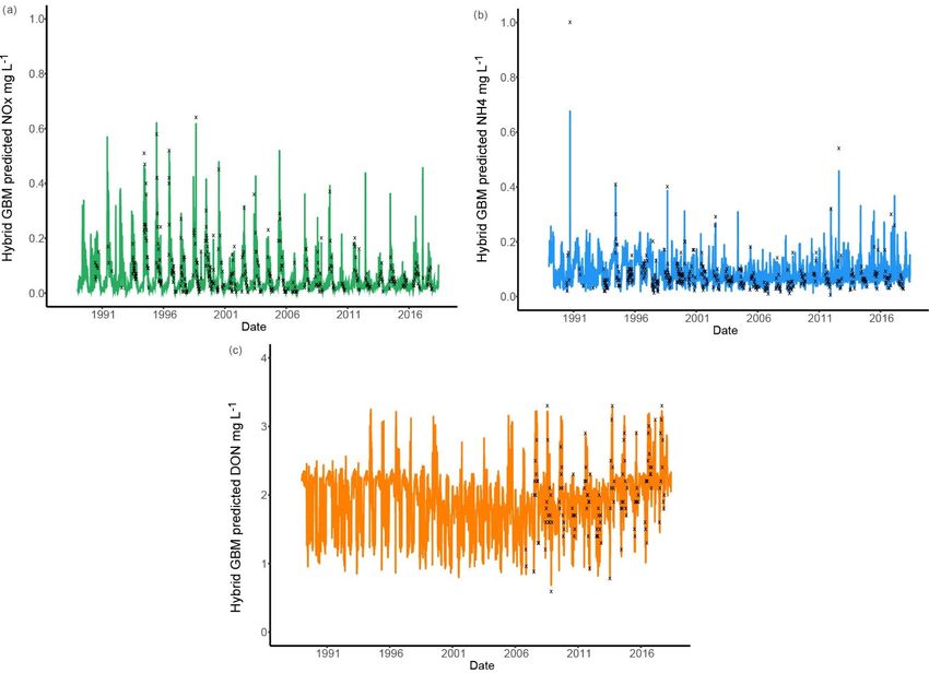
4256                                                                                            B. Wang et al.: ML-SWAN-v1

nodes is calculated for a regression task as                      method was applied for baseflow separation; the quickflow
                                                                  was first estimated as described below (Lyne and Hollick,
          L
          X                R
                           X                                      1979; Nathan and McMahon, 1990), and then baseflow was
error =     (yl − y L )2 +   (yr − y R )2 ,                (4)    calculated:
          l=0              r=0
                                                                                                  1+α
where yl and yr are observations in two split nodes and y L       QFi = αQFi−1 + (Qi − Qi−1 )         ,                       (5)
                                                                                                   2
and y R are the average y in that node. The split is chosen
                                                                  where QFi is the filtered quickflow for the ith sampling in-
among all candidate variables and values to minimise this
                                                                  stant, QFi−1 is the filtered quickflow for the previous sam-
error. This splitting process is applied from the root to the
                                                                  pling instant to i and α is the filter parameter with a value of
terminal node, which creates a tree structure for the model
                                                                  0.925 for daily flow as recommended by Nathan and McMa-
(Erdal and Karakurt, 2013). A CART can be used both for
                                                                  hon (1990). Baseflow is then calculated as BF = Q − QF.
classification and regression problems due to this tree struc-
ture (Coops et al., 2011). However, a single CART can some-       2.4   Performance evaluation metrics
times oversimplify variable interactions and may lead to low
prediction performance (McBratney et al., 2000; Cutler et al.,    In this study, the root mean squared error (RMSE) and
2007; Coopersmith et al., 2010). This drawback can be over-       the Nash–Sutcliffe model efficiency coefficient (MEF) were
come by the ensemble method that generates many resam-            used to compare model performance. The RMSE is a mea-
pled datasets and creates various CARTs to achieve higher         sure of overall error between the predicted and measured data
accuracy (Breiman, 2001) and more stable results when fac-        and returns an error value with the same units as the data,
ing slight variations in input data (Martínez-Rojas et al.,       which is given by the following equation:
2015). New data input is thus evaluated against all trees cre-              s
ated in the ensemble model, and each tree votes using the                      P
                                                                                  (yi − ŷi )2
main class or the averaged values in the terminal node. The       RMSE =                       ,                            (6)
                                                                                     n
class with the maximum votes will be used for a classifica-
tion model, and the averaged predicted value from all trees       where n is the number of data samples. RMSE varies from 0
is used for a regression model (Singh et al., 2014; Belgiu        to +∞, and a perfect model would have RMSE of 0. The
and Drăgu, 2016). It is found that ensemble methods in RF        MEF is a dimensionless “goodness-of-fit” measure which
and GBM can significantly improve the prediction accuracy         can vary from −∞ to 1, with a value of 1 indicating a per-
of CART (Ismail and Mutanga, 2010; Erdal and Karakurt,            fect fit and 0 indicating that the mean of the measured values
2013).                                                            performs as well as the model. The MEF can be calculated
   Compared to LM and WRTDS models, one drawback of               as
RF and GBM, as well as many ML methods in general, is                           P
                                                                                   (yi − ŷi )2
that there is no specific equation in GBM or RF to directly       MEF = 1 − P                   ,                            (7)
demonstrate model structures. However, GBM and RF do                               (yi − y i )2
provide the relative importance of each variable, which is        where y i is the mean of the measured values. Note that the
based on the empirical improvement in the loss function due       predicted and measured nutrient values were normalised to
to the split on the specific variable in a tree (Povak et al.,    [0, 1] in this study to compare model performance across dif-
2014; Puissant et al., 2014). The improvement of a certain        ferent nutrient species.
variable was averaged over all trees and used as the relative
importance of that variable for the final model. This relative    2.5   Overview of modelling processes
importance serves as the key index to understand the model
structure of RF and GBM (Makler-Pick et al., 2011).               The main aims of this research is to test the hybrid model,
                                                                  rebuild the historical nutrient data, and explore the short-
2.3    Baseflow separation                                        and long-term nutrient changes. The first step is verifying the
                                                                  model performance. In this case, the data were randomly di-
Total flow is commonly conceptualised as including baseflow       vided into 80 : 20. Different models were built and tuned on
and quickflow components (Meshgi et al., 2015). Baseflow          the training dataset (80 %) and tested on the testing dataset
separation techniques use the time-series record of stream-       (20 %). To further test model uncertainty and stability, the di-
flow to extract the baseflow and quickflow signatures from        vided and tested processes were repeated 30 times except for
the total flow. This can be done by using graphical methods       WRTDS. After this, all data points including the testing data
to identify the intersection between baseflow and the rising      were then used to rebuild the historical nutrient data. Five-
and falling limbs of the quickflow response (Szilagyi and         fold cross validation (CV) was done on the training dataset
Parlange, 1998) or by filtered methods which process the          to tune the model parameters. Leave-one-out cross validation
entire stream hydrograph to derive a baseflow hydrograph          (LOOCV) was used in WRTDS to predict daily nutrient con-
(Furey and Gupta, 2001). In this study, the three-pass filtered   centrations; LOOCV is the default cross-validation method

Geosci. Model Dev., 13, 4253–4270, 2020                                           https://doi.org/10.5194/gmd-13-4253-2020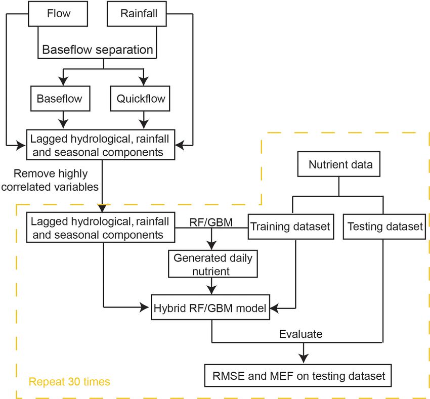
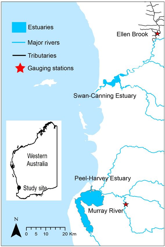
B. Wang et al.: ML-SWAN-v1                                                                                                  4257

in the EGRET (Exploration and Graphics for RivEr Trends)           lagged rainfall data and seasonal components. Note that at
package. In that method, one data point was excluded at a          this stage, the only difference between stand-alone ML and
time from the whole dataset, all other data points were used       hybrid ML methods was that stand-alone ML did not use pre-
to build the model, and the excluded point was used for test-      generated daily nutrient data.
ing the model performance. This process was repeated for
all data points. The performance of all six methods (LM,
WRTDS, RF, GBM, hybrid RF and hybrid GBM) was eval-                3   Site overview
uated on the testing dataset. WRTDS was run through the
EGRET package (Hirsch and De Cicco, 2015) in R to pro-             To test the generalisability of the hybrid framework, two
duce daily concentrations for six nutrient species (TP, TN,        sites in Western Australia (Ellen Brook and Murray River)
DON, DOC, NH4 and FRP). The default settings specified             were selected as study areas. Ellen Brook and Murray River
by the user guide (Hirsch and De Cicco, 2015) were used.           are key tributaries for the Swan–Canning Estuary and Peel–
RF and GBM models were built through the H2 O package in           Harvey Estuary (Fig. 2), respectively, and have different hy-
R.                                                                 drological conditions. The Swan–Canning Estuary is located
   The overall processes of ML-SWAN can be divided into            adjacent to the Perth metropolitan area, with an area of
three stages (Fig. 1). The first stage was baseflow separation     approximately 40 km2 . The catchment comprises 30 catch-
using the EcoHydRology package (Fuka et al., 2018). The            ments, which drain approximately 2090 km2 (Kelsey et al.,
generated baseflow, quickflow, total flow and rainfall were        2010). Ellen Brook is the largest sub-catchment in the Swan–
further transformed into lagged data (the averaged values          Canning catchment, comprising 34 % (716 km2 ) of the total
over the previous 3, 7 and 15 days) to capture any short-term      catchment area. Ellen Brook is an ephemeral river with no
impacts of different water pathways and rainfall on stream         flow recorded during summer and the early autumn months
nutrients. JD, cos(JD) and sin(JD) were also calculated for        (Table 2). The dominant land use in Ellen Brook is agri-
RF and GBM to include seasonal and long-term impacts. A            cultural and grazing land. Ellen Brook is one of the high-
description of all the variables used is given in Table 1.         est contributors of TN and TP to the Swan–Canning Estu-
   The second stage of ML-SWAN was to build intermediate           ary (Swan River Trust, 2009). Bassendean sands and duplex
RF and GBM models that generated daily nutrient concentra-         Yanga (sand over clay) soils dominate the Ellen Brook catch-
tions. For the intermediate RF and GBM models, only lagged         ment. Bassendean sands have very low phosphorus retention
hydrological data (including total flow, baseflow and quick-       indices (PRIs), while Yanga soils have low PRIs in their up-
flow), lagged rainfall and seasonal components on the train-       per horizon and become waterlogged in winter, promoting
ing dataset were used. Nutrients were not used as a predictor      the release of retained nutrients to the stream (Kelsey et al.,
in the intermediate model. Note that, in this study TP, TN,        2010).
DOC and DON were selected to be generated in the second               The Peel–Harvey Estuary is located approximately 75 km
step. If one nutrient was considered as the final target, the      south of the Swan–Canning Estuary, and the Serpentine,
other three nutrients were used to generate daily data. For        Murray and Harvey Rivers drain into the estuary (Fig. 2).
instance, daily TP, DOC and DON were generated as addi-            The total catchment area of the estuary is approximately
tional variables to predict TN. In that case, the missing TP,      11 930 km2 . The Murray River catchment is dominated by
DOC and DON were generated by the intermediate model               deep grey sands, loams clay and peats (Ruibal-Conti et al.,
for the training dataset and the testing dataset. Daily TN, TP,    2013), agricultural land use, and natural reserves, and it con-
DOC and DON data were generated and used for the final             tributes about 40 % of annual TN loads and 7 % of annual TP
predictions. These nutrients were selected since they may          loads to the estuary (Kelsey et al., 2011).
be generated from similar sources or are important compo-             Both Swan–Canning Estuary and Peel–Harvey Estuary
nents of the total nutrient load. For instance, DOC and DON        experience a Mediterranean climate with cool, wet winters
may both be generated from dissolved organic matter (DOM)          (June–August) and hot, dry summers (December–March).
(Seitzinger et al., 2002; Bernal et al., 2005; Filep and Rékási,   The long-term average annual rainfall varies from 1300 mm
2011). In the catchments studied here, DON can be a dom-           on the coast to 800 mm in the south-east of the catchment
inant component of TN (Nice et al., 2009; Petrone, 2010;           area (1975–2009, Bureau of Meteorology station), and about
Bourke et al., 2015). The selection of DOC and DON for             90 % of the rain falls between April and October. Sample
pre-generation may not necessarily be appropriate for other        size and the first measurement year of six nutrients species
catchments. The selection of nutrients for pre-generation de-      are listed for the two study sites in Table 3. TN, TP, NH4
pends on data availability in the dataset. The use of different    and FRP have been monitored for decades, while DOC and
species of the same nutrients (N or P) can generally improve       DON have only been measured in recent years, with limited
model performance.                                                 sample size. Several historical nutrient datasets were com-
   The third stage of ML-SWAN built an additional hybrid           bined but significant changes occurred in water sampling de-
model using the training data, which has generated nutrient        vices and analytical instrumentation over the past decades.
data by the intermediate models, lagged hydrological data,         These changes can increase the complexity of nutrient data.

https://doi.org/10.5194/gmd-13-4253-2020                                             Geosci. Model Dev., 13, 4253–4270, 2020

4258 B. Wang et al.: ML-SWAN-v1
Table 1. Variable list and descriptions.
Variable type Variable name Abbreviation Unit Data source (last access: 9 September 2020)
Hydrological data Total discharge Q m3 s−1 http://wir.water.wa.gov.au
Average total discharge in last x days Qx m3 s−1 Lagged average
Quickflow QF m3 s−1 Equation (5)
Average quickflow in last x days QFx m3 s−1 Lagged average
Baseflow BF m3 s−1 Equation (5)
Average quickflow in last x days BFx m3 s−1 Lagged average
Seasonal components Julian day JD Recorded
Cos (Julian day) cos(JD) Calculated
Sin (Julian day) sin(JD) Calculated
Metrological data rainfall P mm http://www.bom.gov.au
X
P
Cumulated rainfall in last x days P mm Lagged sum
1
Nutrient data Total nitrogen TN mg L−1 http://wir.water.wa.gov.au
Total phosphorus TP mg L−1 http://wir.water.wa.gov.au
Dissolved organic carbon DOC mg L−1 http://wir.water.wa.gov.au
Dissolved organic nitrogen DON mg L−1 http://wir.water.wa.gov.au
Ammonia NH4 mg L−1 http://wir.water.wa.gov.au
Filterable reactive phosphorus FRP mg L−1 http://wir.water.wa.gov.au
Generated dissolved organic nitrogen DONgenerated mg L−1 Generated by the intermediate model
Generated total phosphorus TPgenerated mg L−1 Generated by the intermediate model
Generated dissolved organic carbon DOCgenerated mg L−1 Generated by the intermediate model
Table 2. Hydrological characteristics of the two tributaries.
Site Hydrological type Annual flow (GL) Area (km2 ) Land use
Ellen Brook Ephemeral 26.7 716 Rural, agricultural and grazing
Murray River Perennial 360 7855 Agricultural and natural reserves
For instance, auto-samplers sampled any time regardless of
weather conditions (e.g. during the rainfall), while grab sam-
Table 3. Nutrient sampling time and sample size in Ellen Brook and ples were typically collected under fine weather conditions
Murray River. due to safety concerns.
Site Nutrient First measurement Sample size
4 Results
Ellen Brook TN 1990 1057
TP 1990 1022 4.1 Comparison of prediction accuracy between six
DOC 1995 297
methods
DON 2006 129
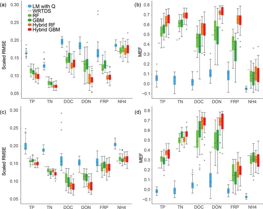
FRP 1990 404
Overall, the scaled RMSE reduced from LM, WRTDS,
NH4 1990 356
stand-alone ML and hybrid ML for all nutrients except NH4 ,
Murray River TN 1983 1648 and the same pattern was found for MEF in both Ellen Brook
TP 1983 1662 and Murray River (Fig. 3). The linear model had the worst
DOC 2006 209 performance: the scaled RMSE was significantly higher and
DON 2006 207 MEF was significantly lower than the other models, for all
FRP 1990 300
six nutrients and across both sites. WRTDS generally had
NH4 1983 570
higher RMSE and lower MEF than the stand-alone ML, al-
though it achieved similar results to stand-alone ML for FRP
and NH4 at both sites. LOOCV was used in WRTDS, and
Geosci. Model Dev., 13, 4253–4270, 2020 https://doi.org/10.5194/gmd-13-4253-2020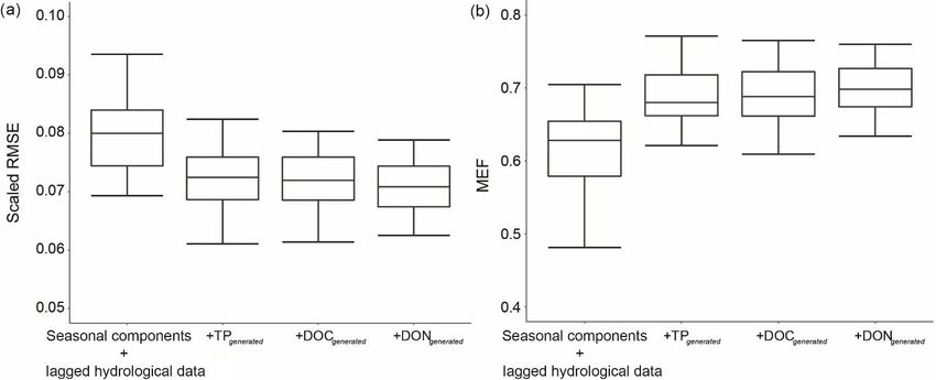
B. Wang et al.: ML-SWAN-v1 4259
Figure 1. Overall modelling processes of ML-SWAN.
only one set of results was generated, compared to 30 RMSE model that allowed more stable results. Interestingly, while
and MEF values for other methods. This results in a short- the hybrid ML had better performance than the stand-alone
ened line for WRTDS in Fig. 3, instead of the interquartile ML, there was no significant difference in performance be-
ranges (IQR = 75th percentile − 25th percentile) presented tween the hybrid RF and hybrid GBM, though they showed
for the other methods. LOOCV can sometimes overestimate differences between different nutrient species. For instance,
the model performance as only one sample was tested at a hybrid RF achieved slightly better performance for DOC in
time; in contrast, 20 % of the independent testing data were Ellen Brook, while hybrid GBM had lower RMSE for DOC
tested in the other five models. LOOCV can also have a in Murray River. There was no significant performance dif-
higher variance than other CV methods (Li, 2016). As such, ference between stand-alone RF and GBM.
the WRTDS results are not directly comparable to the other In summary, the hybrid ML had the best performance
methods. amongst the six methods, followed by stand-alone RF and
Stand-alone ML achieved results that placed it between GBM. WRTDS was better than the linear model but could
WRTDS and hybrid ML. Stand-alone GBM achieved the only achieve results similar to stand-alone RF and GBM for
highest accuracy for NH4 prediction in Murray River. Hy- NH4 prediction in Ellen Brook and for NH4 and FRP predic-
brid RF and hybrid GBM had the lowest RSME and highest tion in Murray River.
MEF for all nutrients except NH4 , in Ellen Brook and Murray
River (Fig. 3). Compared to the stand-alone ML, the hybrid 4.2 Generated daily TN in Ellen Brook
ML also had much lower prediction uncertainty, in that the
RMSE and MEF had narrower IQR than that of the stand- Model performance for six nutrients was compared in the last
alone ML, especially for DON and FRP prediction in Ellen section. To make this section more concise, these six models
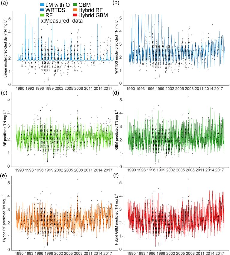
Brook and DOC prediction in Murray River. The use of pre- were then compared in their ability to generate daily TN in
generated daily nutrient data was the only difference between Ellen Brook from 1 January 1989 to 16 July 2018 (Fig. 4).
hybrid ML and stand-alone ML. This means that the gener- The daily TN in Murray River and daily TP in both sites were
ated nutrients provided additional information for the hybrid also generated (see results in the Supplement). TN was se-
lected because TN is the most important and most frequently
https://doi.org/10.5194/gmd-13-4253-2020 Geosci. Model Dev., 13, 4253–4270, 20204260 B. Wang et al.: ML-SWAN-v1
varied in the detail. These models successfully captured the
low-concentration data and the seasonal pattern of TN. Un-
like results by WRTDS, the generated TN by stand-alone ML
and hybrid ML have a more consistent seasonal pattern from
1989 to 2018. The RF and hybrid RF both underestimated
a few high-concentration data (TN < 4.0 mg L−1 ), compared
to GBM and hybrid GBM, although hybrid RF still showed
better performance than RF. For instance, high-concentration
data in 2007 and again from 2014 to 2017 were successfully
predicted by hybrid RF but underestimated by RF. Compared
to stand-alone GBM, the hybrid GBM achieved lower errors
for high-concentration data.
Apart from the better performance for high-concentration
data, another difference between stand-alone ML and hybrid
ML was that the long-term trend in TN was consistent in
stand-alone ML, but this trend fluctuated in hybrid ML. For
instance, hybrid GBM results fluctuated from 1989 to 1999
and then showed an increasing long-term trend from 2005
to 2018, in addition to the seasonal fluctuation. The pre-
generated nutrient is the only difference between stand-alone
model and hybrid model. If there are long-term trends in nu-
trient concentrations (e.g. TN), similar trends should also ex-
ist in the components of TN (either DON or dissolved inor-
ganic nitrogen). The pre-generated nutrients emphasise this
impact on the hybrid model. This suggests that the gener-
ated nutrient data could provide additional information that
allowed the hybrid ML to capture long-term trends; this in-
formation was not included in the seasonal components but
existed in the generated nutrient data.
The distribution of the TN data generated by the six mod-
Figure 2. The location of Ellen Brook and Murray River.
els was compared to the distribution of the measured TN
data (Fig. 5). Similar to the results shown in Fig. 4, hy-
brid GBM had the most similar distribution to the measured
TN data. Only a few low- and high-concentration data were
measured nutrient in many places. This hybrid method can incorrectly predicted by the hybrid GBM. Hybrid RF also
also be used for other nutrients. Note that all data points (not achieved a distribution similar to the measured data, but more
just the 80 % training dataset) were used to generate daily extreme-value data were underestimated compared to the hy-
TN. brid GBM. Stand-alone GBM and RF showed a similar dis-
The LM performed very poorly for TN prediction; low- tribution to the hybrid GBM and RF with less accuracy in
concentration samples (TN < 1.9 mg L−1 ) were all underes- the extreme data. Overall, GBM (either stand-alone model
timated, and some extremely high concentrations were in- or hybrid model) could have a better distribution than RF.
correctly generated due to the high flow (Fig. 4a). There were WRTDS generated some extremely high data and underes-
some seasonal patterns in the generated TN which come from timated many low-concentration data, which is also seen in
the flow data. LM only used total flow to predict nutrient Fig. 4b. The linear model incorrectly predicted most of the
concentrations, while other important hydrological processes TN data. The results in both Figs. 4 and 5 showed that hybrid
were ignored. Thus the oversimplified LM had high errors GBM achieved the best simulated daily TN data, followed
in nutrient prediction (Fig. 4), and this method might be by hybrid RF, stand-alone GBM and RF. WRTDS and LM
more suitable for solutes that are not substantially bioactive generated large biases in TN prediction.
(e.g. SiO2 , Ca2+ , Mg2+ , Cl− ) (Stallard and Murphy, 2014). The hybrid ML models predicted most of the extreme con-
The WRTDS captured some seasonal patterns of TN (from centrations (Figs. 4 and 5), and only a few points were under-
2008 to 2018) but still had problems predicting TN between predicted. The limited number of extreme data and the model
1989 and 1996; some extremely high values were generated, structure that tried to balance the overall trend prediction
and TN < 1.0 mg L−1 were overestimated. Some high val- with extreme data prediction can cause under-prediction. For
ues (e.g. TN in 2008) were underestimated (Fig. 4b). Stand- example, higher weights can be set up for extreme data dur-
alone ML and hybrid ML generated similar daily TN data but ing the model training process to force model to over-predict
Geosci. Model Dev., 13, 4253–4270, 2020 https://doi.org/10.5194/gmd-13-4253-2020B. Wang et al.: ML-SWAN-v1 4261
Figure 3. Model performance across six nutrients and the two sites: (a) RMSE and (b) MEF for Ellen Brook; (c) RMSE and (d) MEF results
for Murray River.
the value for extreme concentrations, which may reduce the The improvement of a certain variable was averaged over all
accuracy for overall trend prediction. In this study, our target trees as the relative importance for the final model. This rela-
is to understand the long-term nutrient trend. Therefore, we tive importance serves as the key index to understanding the
did not use this technique during the model training process. model structure of RF and GBM (Makler-Pick et al., 2011).
The variable importance for TN prediction by hybrid
4.3 Comparison of variable importance in hybrid GBM in Ellen Brook and Murray River is presented in Fig. 6.
GBM for TN prediction The variable importance in the intermediate models is also
included, and the length of coloured sections represents the
The daily data generated by the hybrid GBM showed a lower importance of those variables in the hybrid GBM or interme-
RMSE and better distribution than stand-alone ML, WRTDS diate GBM. The importance was scaled according to the most
and LM (Figs. 4 and 5). Compared to LM, WRTDS and sim- important variable. The generated DON and TP ranked as the
ple CART models, one drawback of RF and GBM, as well first two critical variables in Ellen Brook, while all three gen-
as many ML methods in general, is that there is no specific erated nutrients were listed as the most important variables in
equation in GBM or RF to directly demonstrate model struc- Murray River. This suggests that the generated nutrients do
tures. However, GBM and RF do provide the relative impor- provide critical information to the model and improve model
tance of each variable, which is based on the empirical im- performance. The quickflow was most important for the gen-
provement in the loss function due to the split on the specific erated DON and TP, as well as the TN itself in Ellen Brook.
variable in a tree (Povak et al., 2014; Puissant et al., 2014). The impacts of quickflow decreased, and baseflow, seasonal
https://doi.org/10.5194/gmd-13-4253-2020 Geosci. Model Dev., 13, 4253–4270, 20204262 B. Wang et al.: ML-SWAN-v1
Figure 4. Daily TN generated by the six models for Ellen Brook.
components and rainfall data become more important for TN 5 Discussion
prediction in Murray River. This difference in variable im-
portance reflects different catchment characteristics across 5.1 Different sources of TN in Ellen Brook and Murray
the two sites and therefore different hydrological and hydro- River
chemical processes controlling TN concentrations. The total
flow was not of high importance at either site, which suggests Hydrological conditions, specific sub-catchment character-
that baseflow or quickflow had more impact on surface wa- istics and the chemical properties of nutrients can all im-
ter TN. Moreover, TN concentrations were affected by more pact surface water nutrient concentrations (Barron et al.,
variables in Murray River than in Ellen Brook. 2009; Moatar et al., 2016), nutrient partitioning (Ruibal-
Conti et al., 2013) and nutrient transport (Burt and Pinay,
2005; Tesoriero et al., 2009). TN prediction in Murray River
was impacted by more variables than in Ellen Brook (Fig. 6),
suggesting more complex relationships in Murray River.
Geosci. Model Dev., 13, 4253–4270, 2020 https://doi.org/10.5194/gmd-13-4253-2020B. Wang et al.: ML-SWAN-v1 4263
important variable for TN prediction in Murray River. The
Murray River catchment has large areas with high nutrient-
retaining soils (high PRI) (Kelsey et al., 2011) and rela-
tively low TN concentrations, and it is likely that ground-
water makes significant contributions to TN in Murray River.
Ruibal-Conti et al. (2013) previously found that variability in
TN is strongly associated with variability in flows in Murray
River. Our results extend this finding, in that both baseflow
and quickflow likely impact TN in the river.
It is noted that seasonal components including sin(JD),
and cos(JD) showed significantly higher importance in Mur-
ray River. This may because seasonal information is captured
in other inputs in Ellen Brook (e.g. quickflow and baseflow).
But the main reason is the stronger seasonal TN signals in
Murray River compared to Ellen Brook. This finding is sup-
Figure 5. The distribution of the daily TN generated by the six mod-
ported by the generated daily TN data for Murray River (see
els and that of the measured TN data in Ellen Brook.
results in Supplement S2). Natural reserves occupy large ar-
eas of the Murray River catchment, and this may increase
seasonal signals. Additionally, the lagged quickflow, base-
Quick flow is composed of runoff, interflow and direct pre- flow and rainfall were generated (for the previous 3, 7 and
cipitation (Brodie and Hostetler, 2005) and was shown to be 15 days), but only the lagged 15 d baseflow and quickflow
important for TN prediction in Ellen Brook. Direct precipita- were ranked as important variables for both Ellen Brook and
tion, however, did not have a large impact on TN (the green Murray River. This suggests a timescale of nutrient trans-
bars in Fig. 6); this suggests that runoff and interflow were port in the sub-catchments and likely reflects soil permeabil-
important for TN concentrations. Baseflow can account for ity and geology; long hydrochemical recessions from storm
(on average) 53 % of annual stream discharge in Ellen Brook, events may prolong their impact on the ecological status of
but baseflow was not of high importance for TN prediction in receiving rivers (Mellander et al., 2012).
this study. This may occur due to low TN concentrations in Six models were compared for nutrient predictions and the
the baseflow (Barron et al., 2009), large areas of low nutrient- hybrid GBM model achieved the highest accuracy (Figs. 3
retaining sandy soils in the Ellen Brook catchment, and high and 5). The long-term changes in TN have been discussed
nutrient transport efficiency in quickflow and first flush. Mel- in previous sections. To understand the long-term changes in
lander et al. (2012) quantified nutrient transport pathways in other nitrogen species across the year, the hybrid GBM was
agricultural catchments and found that quickflow was only then applied to generate daily DON, NH4 and NOx in Ellen
2 %–8 % of total flow, but it can transport up to 50 % of TP. Brook from 1 January 1989 to 16 July 2018 (Fig. 7). The gen-
Gunaratne et al. (2017) found that the seasonal first flush was erated DON has much higher concentration than NH4 and
only 30 % of runoff volume but contained 40 %–70 % of the NOx . This is consistent with previous investigations in this
nutrient load. study area that DON was the dominant form of TN in both
Note that the median TN in Ellen Brook (2.1 mg L−1 ) is surface water and groundwater (Nice et al., 2009; Petrone,
significantly higher than that in Murray River (0.67 mg L−1 ) 2010; Bourke et al., 2015). There is no clear long-term pat-
which can be explained to some extent by the large area terns in generated NH4 and NOx ; however, an increasing
of grazing lands in Ellen Brook. Previous investigations in long-term trend in generated DON can be found from 2006
south-eastern Australia (Adams et al., 2014), New Zealand to 2018. There is also an increasing trend in TN from 2005
(Davies-Colley et al., 2004) and north-western Europe (Con- (Fig. 4), suggesting DON was the main reason for the in-
roy et al., 2016) all suggested that livestock can increase TN creasing TN concentrations. DON is often assumed to be rel-
discharge to the receiving water bodies. Most of the piggeries atively slow to react, but depending on the source of DON, it
and poultry farms in the Swan–Canning catchment are lo- can turnover rapidly, thereby constituting an active contrib-
cated in Ellen Brook catchment (Kelsey et al., 2010), which utor to the eutrophication of surface waters (Petrone et al.,
has the highest TN and TP discharge loads. Thus the large 2009).
grazing areas, piggeries and poultry farms and low nutrient-
retaining sandy soils may explain the importance of quick- 5.2 Can we improve our understanding of historical
flow for TN prediction and high TN concentrations in Ellen nutrient conditions using a contemporary data?
Brook.
Baseflow is derived from groundwater discharge to The generated nutrient data provided additional information
streams and the slow drainage of water stored in local wet- to enhance the hybrid model performance (Figs. 3 and 5). To
lands (Kelsey et al., 2010). Baseflow is highlighted as an assess the individual impact of a generated nutrient, we did
https://doi.org/10.5194/gmd-13-4253-2020 Geosci. Model Dev., 13, 4253–4270, 20204264 B. Wang et al.: ML-SWAN-v1
Figure 6. Variable importance in the hybrid GBM for TN prediction in (a) Ellen Brook and (b) Murray River.
a simple test that sequentially added generated TP, DOC and Our results suggest that the recent DON and DOC data
DON data to the base GBM (only seasonal components and improved understanding of historical TN. It is not uncom-
lagged hydrological data) and evaluated RMSE and MEF for mon to have a similar data structure when several datasets
TN prediction. This process was repeated 30 times and the are combined or new measurements are added to a project.
results are presented in Fig. 8. While there were no DON data prior to 2006 in Ellen Brook,
The RMSE significantly decreased when generated TP daily DON can be generated back to 1990 with the help of
was added as an additional variable. DOC and DON only generated TN, DOC and TP data; DON had the highest MEF
have 297 and 129 data, respectively, and were only measured among the six nutrients (Fig. 3). This hybrid method pro-
in recent years, while TP has more than 1000 data and has vides a feasible process to fully utilise all available nutrient
been measured since 1990 (Table 3). However, DOC and data to accurately fill gaps in either historical or recent nutri-
DON could still improve model performance (Fig. 8), and ent datasets.
the generated DON was ranked as the most important vari-
able across both sites (Fig. 6). The medium RMSE slightly 5.3 A comprehensive comparison of six models
decreased when both generated DOC and DON were added.
Moreover, the generated DOC and DON also reduced the Monitoring, modelling and forecasting water quality inputs
model uncertainty, such that the IQRs became narrower than are essential to support the management of the quality of
model results without the generated nutrients. receiving waters while responding to current anthropogenic
stressors (Holguin-Gonzalez et al., 2013; Schnoor, 2014).
Geosci. Model Dev., 13, 4253–4270, 2020 https://doi.org/10.5194/gmd-13-4253-2020B. Wang et al.: ML-SWAN-v1 4265 Figure 7. Generated daily DON, NOx and NH4 by the hybrid GBM for Ellen Brook. Figure 8. Model performance for TN prediction across different input variables for Ellen Brook. https://doi.org/10.5194/gmd-13-4253-2020 Geosci. Model Dev., 13, 4253–4270, 2020
4266                                                                                           B. Wang et al.: ML-SWAN-v1

The performances of six models were comprehensively com-          understanding on which to base the selection of the impor-
pared, in an exploration of historical and contemporary nu-       tant variables.
trient data across two study sites. LM had the highest error         In this study, we tested the generalised performance of the
while stand-alone RF and GBM had similar error. This agrees       hybrid model across six nutrient species and two tributaries.
with previous findings by Erdal and Karakurt (2013) that RF       We also note that nutrients may not always be the critical
and GBM models achieved similar correlation coefficients          variables targeted for pre-generation; the pre-generated DOC
(R) for streamflow forecasting. Ismail and Mutanga (2010)         was ranked as having low importance for Ellen Brook and
also reported that RF and GBM increased the R of a single         produced only a slight improvement in the performance of
CART by 10.01 % and 9.59 %, respectively.                         the hybrid model for NH4 .
   The performance of WRTDS, as well as many conceptual
models, is often reliant on a prescribed set of input infor-      5.4    The application of ML methods for hydrological
mation, which can account for variance in nutrient concen-               modelling
trations but may miss some important processes for certain
rivers (e.g. baseflow in this study). This can compromise the     There were constraints in the nutrient datasets in this re-
performance of WRTDS for nutrient prediction. Moreover,           search, and similar constraints commonly exist in other study
hydrological and chemical processes within the systems are        areas. Many nutrient datasets contain important information,
typically ignored by many conceptual models, which may            but sometimes it can be challenging to directly combine or
exclude important hydrochemical information. By contrast,         utilise them. ML methods provide a feasible approach to
some complex conceptual models may include these hydro-           preprocess these datasets or combine them. In this study,
chemical processes but are often constrained by insufficient      the concentrations of missing nutrient species were first pre-
nutrient data to calibrate and validate the models. Some sim-     dicted by the intermediate ML method and then used as in-
plifications may be made to account for lack of data, but the     puts for another ML method for final predictions. The pre-
simplifications may often weaken model performance. The           generation of missing data and pre-modelling hydrological
hybrid framework presented in this study has overcome the         analysis were critical components of the hybrid model and
challenge caused by data paucity by building intermediate         allowed the identification of the impact of different hydrolog-
models to generate missing nutrient data and then using this      ical transport pathways for TN export from the two tributary
additional hydrochemical information to improve final model       catchments. The hybrid ML methods were further applied to
performance.                                                      generate nutrient data for eight tributaries, and the generated
   The hybrid models developed in this study were able to         data have since been used as inputs to an estuary prediction
take advantage of the complementary strengths of both hy-         model, which simulates and forecasts nutrient concentrations
drochemical (additionally generated nutrient data) and hy-        in the previous and next 5 d in the Swan–Canning Estuary
drological (lagged data) information. This was particularly       (Huang et al., 2019). The modelling methods and strategies
the case for the prediction of high nutrient concentrations,      developed in the work presented here can be easily applied
where the hybrid models were shown to outperform the              to other study areas. Overall, ML methods provide a flexible
stand-alone RF and GBM, in terms of accuracy, reliabil-           and feasible solution to explore the underlying relationships,
ity and value distribution. Improved accuracy in the hybrid       reconstruct spatial and temporal datasets, and combine dif-
model was achieved by using intermediate models, although         ferent models.
these intermediate models may also have a relatively high
error (similar to stand-alone RF and GBM). However, if
the improved model performance is higher than the intro-          6     Summary and conclusion
duced error, the results are manageable. Similar results were
also found in Hunter et al. (2018), who compared a hybrid         A hybrid machine learning model was developed, and its per-
process-driven and ANN model with the stand-alone ANN             formance tested on six nutrients and two estuary tributaries
model and the process-driven model. In their study, the hy-       and compared with alternative modelling approaches. The
brid also achieved the best performance followed by stand-        hybrid ML model exhibited higher prediction accuracy and
alone ANN. The process-driven benchmark model had a sig-          lower prediction uncertainty than stand-alone ML, WRTDS
nificantly lower accuracy than the other two models.              and LM for almost all nutrients. The pre-generation of miss-
   A limitation of the hybrid modelling approach, however, is     ing data and pre-modelling hydrological analysis were criti-
that it requires the time and expertise to develop intermediate   cal components of the hybrid model and allowed the iden-
models for generating additional nutrient data. Prior knowl-      tification of the impact of different hydrological transport
edge also plays an important role in identifying the variables    pathways for TN export from the two tributary catchments.
for pre-generation. Some statistical methods (e.g. the corre-     The results of this study demonstrate the advantages of using
lation test, simple linear model) can be helpful to identify      hybrid models for high temporal resolution nutrient predic-
these variables if there is no clear theoretical or conceptual    tion; the results also demonstrate the use of the hybrid model
                                                                  for re-analysis of historical data in the light of contemporary

Geosci. Model Dev., 13, 4253–4270, 2020                                           https://doi.org/10.5194/gmd-13-4253-2020
B. Wang et al.: ML-SWAN-v1 4267
data. Modelling strategies for different modelling targets and ments in south-east Australia, J. Hydrol., 515, 166–179,
dataset structures have also been discussed. The modelling https://doi.org/10.1016/j.jhydrol.2014.04.034, 2014.
framework presented here can aid others to fully use all avail- Álvarez-Cabria, M., Barquín, J., and Peñas, F. J.: Modelling
able nutrient data to generate accurate nutrient predictions. the spatial and seasonal variability of water quality for
entire river networks: Relationships with natural and an-
thropogenic factors, Sci. Total Environ., 545–546, 152–162,
https://doi.org/10.1016/j.scitotenv.2015.12.109, 2016.
Code and data availability. The data and the data sources used in
Barron, O., Donn, M., Furby, S., Chia, J., and John-
this study are cited and explained in the text. The current version
stone, C.: Groundwater contribution to nutrient ex-
of model is available from the project website: https://github.com/
port from the Ellen Brook catchment, available at:
benyawang-uwa/daily-nutrient-prediction (last access: 9 Septem-
http://www.clw.csiro.au/publications/waterforahealthycountry/
ber 2020) under the MIT licence. The exact version of the model
2009/wfhc-groundwater-Ellen-Brook-catchment.pdf (last
used to produce the results used in this paper is archived on Zenodo
access: 9 September 2020), 2009.
(https://doi.org/10.5281/zenodo.3739611, Wang, 2020).
Belgiu, M. and Drăgu, L.: Random forest in remote sens-
ing: A review of applications and future directions,
ISPRS J. Photogramm. Remote Sens., 114, 24–31,
Supplement. The supplement related to this article is available on- https://doi.org/10.1016/j.isprsjprs.2016.01.011, 2016.
line at: https://doi.org/10.5194/gmd-13-4253-2020-supplement. Bernal, S., Butturini, A., and Sabater, F.: Seasonal variations
of dissolved nitrogen and DOC : DON ratios in an inter-
mittent Mediterranean stream, Biogeochemistry, 75, 351–372,
Author contributions. BW, MRH and CO contributed to the devel- https://doi.org/10.1007/s10533-005-1246-7, 2005.
opment of the methodology and designed the experiments, and BW Bourke, S., Hammond, M., and Clohessy, S.: Perth Shallow
carried them out. BW developed the model code and performed Groundwater Systems Investigation: North Lake, available at:
the simulations. BW prepared the paper with contributions from all https://www.water.wa.gov.au/__data/assets/pdf_file/0016/7432/
coauthors. 108960.pdf (last access: 9 September 2020), 2015.
Breiman, L.: Random forests, Mach. Learn., 45, 5–32, 2001.
Breiman, L., Friedman, J., Stone, C. J., and Olshen, R. A.: Classifi-
Competing interests. The authors declare that they have no conflict cation and regression trees, CRC Press, Boca Raton, 1984.
of interest. Brodie, R. and Hostetler, S.: A review of techniques for analysing
baseflow from stream hydrographs, in: Proceedings of the
NZHS-IAHNZSSS 2005 Conference, Auckland, New Zealand,
Acknowledgements. The authors acknowledge Peisheng Huang and 2005.
Brendan Busch for providing the historical nutrient data. Burt, T. P. and Pinay, G.: Linking hydrology and
biogeochemistry, Prog. Phys. Geogr., 3, 297–316,
https://doi.org/10.1067/mva.2002.123763, 2005.
Financial support. Benya Wang was supported by a postgradu- Chanat, J. G., Rice, K. C., and Hornberger, G. M.: Consistency of
ate scholarship provided by the CRC for Water Sensitive Cities. patterns in concentration-discharge plots, Water Resour. Res., 38,
Matthew R. Hipsey received funding support from the Australian 10–22, https://doi.org/10.1029/2001WR000971, 2002.
Research Council (project LP150100451). Chen, Y., Liu, R., Sun, C., Zhang, P., Feng, C., and Shen, Z.: Spatial
and temporal variations in nitrogen and phosphorous nutrients
in the Yangtze River Estuary, Mar. Pollut. Bull., 64, 2083–2089,
https://doi.org/10.1016/j.marpolbul.2012.07.020, 2012.
Review statement. This paper was edited by Thomas Poulet and re-
Clapcott, J. E., Collier, K. J., Death, R. G., Goodwin, E. O.,
viewed by Thu Huong Thi Hoang and one anonymous referee.
Harding, J. S., Kelly, D., Leathwick, J. R., and Young, R.
G.: Quantifying relationships between land-use gradients and
structural and functional indicators of stream ecological in-
tegrity, Freshw. Biol., 57, 74–90, https://doi.org/10.1111/j.1365-
References 2427.2011.02696.x, 2012.
Cohn, T. A., Delong, L. L., Gilroy, E. J., Hirsch, R. M., and Wells,
Abbott, B. W., Baranov, V., Mendoza-Lera, C., Nikolakopoulou, D. K.: Estimating constituent loads, Water Resour. Res., 25, 937–
M., Harjung, A., Kolbe, T., Balasubramanian, M. N., Vaessen, 942, https://doi.org/10.1029/WR025i005p00937, 1989.
T. N., Ciocca, F., Campeau, A., Wallin, M. B., Romeijn, P., Conroy, E., Turner, J. N., Rymszewicz, A., O’Sullivan, J. J., Bruen,
Antonelli, M., Gonçalves, J., Datry, T., Laverman, A. M., M., Lawler, D., Lally, H., and Kelly-Quinn, M.: The impact of
de Dreuzy, J. R., Hannah, D. M., Krause, S., Oldham, C., cattle access on ecological water quality in streams: Examples
and Pinay, G.: Using multi-tracer inference to move beyond from agricultural catchments within Ireland, Sci. Total Environ.,
single-catchment ecohydrology, Earth-Science Rev., 160, 19–42, 547, 17–29, https://doi.org/10.1016/j.scitotenv.2015.12.120,
https://doi.org/10.1016/j.earscirev.2016.06.014, 2016. 2016.
Adams, R., Arafat, Y., Eate, V., Grace, M. R., Saffarpour, Coopersmith, E. J., Minsker, B., and Montagna, P.: Un-
S., Weatherley, A. J., and Western, A. W.: A catch- derstanding and forecasting hypoxia using machine
ment study of sources and sinks of nutrients and sedi-
https://doi.org/10.5194/gmd-13-4253-2020 Geosci. Model Dev., 13, 4253–4270, 2020You can also read