On the response of tidal rivers to deepening and narrowing - Risks for a regime shift towards hyper-turbid conditions. J.C. Winterwerp March 2013
←
→
Page content transcription
If your browser does not render page correctly, please read the page content below
i

On the response of tidal rivers
to deepening and narrowing

Risks for a regime shift towards hyper-turbid conditions.

J.C. Winterwerp

March 2013
ii

DISCLAIMER:

This is the report as it was delivered in January 2013 to the clients. After discussions on
all the results of the research program 'LTV Safety and Accessibility' with various
stakeholders in the Flemish-Dutch Scheldt Committee a final version of the report is
made
iii

Table of contents

1.    Introduction

2.    Tidal evolution in a converging estuary with intertidal area
 2.1 Derivation of the relevant equations
 2.2 The response of an estuary to deepening and narrowing

3.    Fine sediment transport in narrow estuaries
 3.1 Transport components
 3.2 Reduction in effective hydraulic drag
 3,3 Hyper-concentrated conditions
 3,4 A qualitative description of the regime shift in the Ems estuary

4.    Comparison of various estuaries
 4.1 The Ems River
 4.2 The Loire River
 4.3 The Elbe River
 4,4 The Weser Estuary
 4.5 The Upper Sea Scheldt

5.    Summary and conclusions

6.    Recommendations

      Acknowledgments

      References

      Notation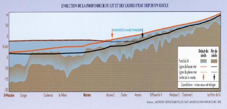
1

1. Introduction

Fig. 1.1 depicts the evolution of the tidal range over roughly the last century in five European
ports, which are all situated more than 50 km from the mouth of fairly small and narrow estuaries.
It is generally accepted that this large tidal amplification is caused by the ongoing deepening and
canalization of these rivers, accommodating ever-larger ships; though the precise mechanisms
behind are not yet understood. Of course, the increases in high water levels, and decreases in low
water levels form serious problems by themselves, e.g. enhanced flood levels, salinity intrusion,
and lowering of ground water table. However, it becomes more and more evident that such
deepening and narrowing induce large environmental problems as well. Infamous are the Ems
(Germany) and Loire (France) Rivers. Today, both rivers can be characterized as hyper-turbid,
with suspended sediment (SPM) concentrations of several 10 g/l, and large-scale occurrences of
fluid mud. Strong vertical stratification causes serious water quality problems, and in the Loire
the enhanced salinity intrusion yields problems with fresh water intake for industry and
agriculture. The causes of the evolution of Loire and Ems to these hyper-turbid states are not yet
fully understood (Talke et al, 2008 & 2009; Chernetsky, 2010; Winterwerp, 2011), though there
is consensus that the large amplification of the tidal range must have played an important role.

                                                 summary tidal evolution
                                   6
                 tidal range [m]

                                   4

                                                                              Antwerp
                                   2                                          Bremen
                                                                              Hamburg
                                                                              Nantes
                                                                              Papenburg
                                   0
                                   1875   1900   1925     1950       1975   2000     2025
                                                           year

Fig. 1.1: Tidal evolution in five European ports (Antwerp along Scheldt, Belgium; Bremen along
Weser, Germany; Hamburg along Elbe, Germany; Nantes along Loire, France; and Papenburg along
Ems, Germany).

Also the Scheldt-estuary is renown for its long lasting human interventions, such as deepening,
narrowing by embankments (land reclamations, and loss of intertidal area), sand mining and
large-scale sediment displacements by dredging and dumping. As authorities fear an evolution
such as in the Ems and Loire Rivers, the Flemish Department of Maritime Access initiated the
current study, which is carried out in the framework of a larger research program on the Scheldt
estuary.

This study is based on a comparison of the analysis of historical tidal data of four rivers, e.g.
Elbe, Ems, Loire and Scheldt. This analysis is carried out with a simple analytical model, which
describes the solution of the linearized shallow water movement equations. The derivation of this
model is presented in Chapter 2, together with a conceptual analysis of the response of a tidal
river to deepening and narrowing (loss of intertidal area). Chapter 3 describes the interaction of
fine suspended sediment with the turbulent water movement, which may result in a considerable
reduction in effective hydraulic drag. Also we introduce the conditions which may lead to a
secondary turbidity maximum, and arguments that hyper-turbid conditions are favorable from an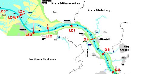
2

energetic point of view. The actual analysis of the historical tidal data is carried out in Chapter 4,
where we establish the evolution of the tidal damping in the rivers as a function of changes in the
river’s geometry and bathymetry, discussing the role of tidal reflection and reductions in effective
hydraulic drag. The results of the individual rivers are compared in Chapter 5, presenting a
conceptual diagram on the evolution of a tidal river towards hyper-turbid conditions in response
to human interventions.
3
2. Tidal evolution in a converging estuary with intertidal area
2.1 Derivation of the relevant equations
the equations
In this section, we derive the dispersion equation for tidal propagation in a converging estuary
with a compound cross section, e.g. Fig. 2.1.
Fig. 2.1: Compound channel and definitions.
We follow Friedrichs (2010) and Dronkers (2005), but make no a priori assumptions on the
contribution of the various terms in the equations, except for a linearization of the friction term,
and we neglect the advection term in the momentum equation:
Acu
bc b 0
t x
(1)
u ru
g 0
t x h
We refer to Dronkers (1964) for a complete analysis of these equations in a straight channel. Here
we focus on a converging estuary, as almost all natural, alluvial estuaries are characterized by a
so-called trumpet shaped plan form (e.g. Prandle, 2004). If we assume Ac hbc , equ. (1) can be
re-written as:
Ac u 1 bc 1 h Ac
u0 (2a)
t bc b x bc x h x bc b
u ru
g 0 (2b)
t x h
where = instantaneous water level, u = cross-sectionally averaged flow velocity, h = tidal-mean
water depth, bc = width flow-carrying cross section, b = width intertidal area (over which the
flow velocity is zero), Ac = surface area flow-carrying cross section Ac hbc , assuming 0 up-estuary). We focus on exponentially converging estuaries, e.g.
bc b0 exp x Lb , where b0 = width flow-carrying cross section in the mouth of the estuary4
and Lb = convergence length (typical values between ~20 and ~40 km). The drag coefficient cD
attains values of 0.001 to 0.003 m/s (corresponding Chézy values of 100 – 60 m1/2/s, as
r gU C 2 ), hence r also varies from around 0.001 to 0.003. In the following, we assume that
the river flow is so small that its effects can be neglected. Finally, further to our linear approach,
we also assume that parameters may vary along the estuary, such as the tidal amplitude, but that
these variations are relatively small, and that the tidal amplitude is small compared to the water
depth.
If we neglect longitudinal gradients in tidal-mean water depth h x , the continuity and mass
balance equation read1):
Ac u Ac u
0 (3a)
t bc b x bc b Lb
u ru
g 0
t x h (3b)
the dispersion relation and wave numbers
We assume that the solution to (3) follows a harmonic function:
x, t h a0 exp i t kx and u x, t U 0 exp i t kx (4a)
where a0 = tidal amplitude at x = 0, U0 = amplitude flow velocity at x = 0, = tidal frequency;
= 2T ; T = tidal period, k = complex wave number; k = kr + iki, kr = real wave number (kr =
2/), = tidal wave length, ki = imaginary wave number, and = phase angle between tide and
velocity. Note that the three unknowns a0, U0 and are real. Next, we substitute (4a) into (3a)
and (3b):
Ac Ac 1
i a0 ik U 0 exp i 0 (5a)
bc b bc b Lb
r
igka0 i U 0 exp i 0 (5b)
h
From equ. (5b) we can derive the velocity amplitude U0 as a function of a0:
igka0 ga0 kr2 ki2
U 0 mod (5c)
i r* exp i r*2 1
1)
Note that a more general derivation is obtained by assuming an exponentially converging cross section;
however, it is difficult to account for spatially varying water depth. To account for longitudinal variations
in water depth as good as possible, the rivers are sub-divided into sub-sections with constant depth in our
analyses below (see f.i. Jay, 1991).5
equ’s (5a) and (5b) can be written in matrix form:
Ac Ac 1
i ik exp i
bc b bc b Lb a0 0 (6)
r U 0
igk i exp i
h
Requiring the existence of non-trivial solutions yields a dispersion equation implicit in the wave
number k:
r Ac Ac 1
i i igk ik 0
h bc b bc b Lb
or 2 2i e 1 ir* 0 (7)
bc b r
Lb k 2 ik Lb 2 1 i 0
ghbc h
in which the following dimensionless parameters have been defined:
r i i 2 kr iki Lb 2kLb
2 Lb 2 Lb gh
L* , where Lg
gh Lg
r gU
r*
h hC 2 (8)
b b
b* c
bc
bc b 4 L2b 2 4 L2b 2
e b L 2
* *
bc gh gAc btot
Here we introduce the estuarine convergence number e, through which all geometrical and
bathymetrical features of the rivers are accounted for. Note that e decreases with increasing
water depth, increasing convergence of the river’s plan form, and decreasing intertidal area. Next,
from (7) k is resolved:
bc b 2 2 b b 2 r
1 1 4 Lb 4 c Lbi
gAc gAc h 1 1 e i e r* (9)
k1,2 i i
2 Lb 2 Lb
Using MAPLE, the real and imaginary part of (9) are determined:6
2 2
1 L2b 2 L2b 2 r
2
kr 2 4 1 b bc 1 4 1 b bc
4 Lb gh gh h
12 (10a)
L2 2
2 4 1 b bc b 1
gh
2 2
1 L2b 2 L2b 2 r
2
1
ki 2 4 1 b bc 1 4 1 b bc
2 Lb 4 Lb gh gh h
(10b)
12
L
2
2
2 4 1 b bc b
1
gh
The positive and negative real wave numbers represent the up-estuary propagating tidal wave,
and its reflection, if any. We note that the imaginary wave number for the up-estuary propagating
wave differs from its reflection, which is to be attributed to the funnel shape of the estuary. This
explains why i is always positive, i.e. the reflected tidal wave is always damped. Indeed, when
Lb = , as in the case of a straight, prismatic channel, all wave numbers become symmetric again.
For a non-converging (Lb = ), frictionless channel (r = 0), equ. (10) converges to the well-
known relations kr bc b bc gh and ki = 0. For a non-converging channel with friction,
we obtain:
b* 2 12
b* 2 12
kr 1 r*2 1 and ki 1 r*2 1 (10c)
2 gh 2 gh
In dimensionless form, the wave numbers (10) for the up-estuary propagating wave, and its
reflection, represented by the superscripts ▪+ and ▪-, respectively, read:
12
r 2 e 1 e r* 2 e 1 and
1 2 2
2 (11a)
12
r 2 e 1 e r* 2 e 1
1 2 2
2
12
i 1 2 2 e 1
1
e 1 e r*
2 2
and
2
(11b)
12
1 2 2 e 1
1
e 1 e r*
2 2
2
i
In the remainder, we will work with both the dimensionless and non-dimensionless equations.
However, we will use the dimensionless parameters of equ. (8) comparing the various estuaries in
Section 4 of this report.7
limiting values of the wave numbers
Let us analyze these solutions for a converging estuary with a rough, frictionally-dominated bed
(r = ) and for an estuary with a very smooth bed, formed by fluid mud ( r ≈ 0). In the first case
the friction term dominates the expression below the square root-sign, in the second case, friction
can be neglected. The real and imaginary wave number for a frictionless system read (assuming
shallow water, i.e. h not too large)
r r 0
e 1 and i r 0 1 (12a)
Equ. (12) shows that for a smooth bed, the tidal wave is amplified with the convergence length
Lb; this is therefore the maximum amplification of the tide according to linear theory. In case of a
rough bed (r = ), the real and imaginary wave number become:
1
kr r
2 e r* or r r
e r* 2
4 Lb
(12b)
1
ki r
2 e r* or i r
e r* 2
4 Lb
The phase angle between tidal elevation and velocity follows from substitution of (4a) into (3a),
elaborating the real part only:
Ac Ac 1
i a0 i kU 0 exp i U 0 exp i 0 (5a)
bc b bc b Lb
Lb ki 1 i 2
tan (13a)
Lb kr r
Substituting from (12) yields the phase angle for a smooth and friction dominated system:
1 e r* 8
tan r 0 and tan r 1 (13b)
e 1 e r*
The celerity c of the tidal wave into the estuary is given by:
2 Lb
c (14a)
kr r
Substituting from (12) yields the celerity for a smooth and friction dominated system:8
2 Lb 8 Lb
c r 0 and c r (14b)
e 1 e r*
the general solution
Next, we study the propagation and amplification/damping of the tide in an infinitely long estuary
and/or an estuary of finite length ℓ (for instance by a weir at x = ℓ). In dimensionless form, the
length of the estuary then measures r = ℓ/2Lb. At the mouth of the estuary we prescribe a simple
cosine tide:
0, t h a0 cos t (15)
in which a0 = amplitude of the tide. Next, we introduce its complex equivalent x, t and
require that Re 0,t a0 . The harmonic solution to equ. (3) then reads:
x, t h a0 exp i t k x a0 exp i t k x and (16a)
u x, t U
0 exp i t k x U exp i t k x
0
in which a and a are the amplitudes of the incoming and reflecting tidal wave. In case of an
infinitely long river, equ. (16a) reduces to:
x, t h a0 exp i t kx and
(16b)
u x, t U 0 exp i t kx
as in equ. (4a). The boundary conditions to the solution of equ.’s (3) and (16a) are given by:
x = 0: a0 a0 a0 ,
x = ℓ: U 0 , hence U U .
Further to equ. (3b), the latter implies that
x = ℓ: a x a x , so that a0 k exp ik a k
0
exp ik 0.
Hence, we find for the two amplitudes a0 and a0 from the modulus of a0:
k exp ik
k exp ik exp ik x
a a0 ; a a0 (17a)
k exp ik k exp ik k exp ik k exp ik
0
k exp ik
k exp ik exp ik x a
a a0 ; a
k exp ik k exp ik k exp ik k exp ik
0 0 (17b)9
resonance of the tidal wave
As k kr iki kr i p q and k kr iki kr i p q , where p and q are
dummy variables, we can re-write (17) as:
k exp ikr
a a0 (18a)
k exp ikr k exp ikr exp 2q
0
k exp ikr exp 2q (18b)
a a0
k exp ikr exp 2q k exp ikr
0
Hence, lim a0 a0 and lim a0 0 , retrieving the simple propagating wave in an infinitely
long converging estuary. Furthermore, equ. (17) shows that resonance can occur when:
Re k exp ik k
exp ik 0 , i.e
kr exp ki k exp ki
tan kr n
r
or
2 ki exp ki k i
exp k
i
(19a)
r exp i r r exp i r
tan r r n
2 i exp i r i exp i r
As equ. (19) is implicit in , we cannot determine the conditions for resonance analytically.
However, for a straight channel, ki ki (e.g. equ. (11b), tan kr , which is the case if
4 , where = wave length in a straight frictionless channel, e.g. Dronkers (1964). For a
very strong converging channel, e.g. lim kr lim ki lim ki 1 , tan kr 1 , and 8 .
Lb 0 Lb 0 Lb 0
Of course, the wave length in a straight and very converging channel are very much different (in
fact if Lb = 0, = 0).
The solution to equ. (19) is depicted graphically in Fig. 2.2. Note that typical values for e
range from 1 to 2 (e.g. Chapter 4).10
resonance in converging estuaries
6
r* = 1 (muddy bed)
5
r* = 3
r* = 6 (sandy bed)
4
krℓ [-] 3
2
1
0
0 2 4 6 8 10
estuarine convergence number e [-]
Fig. 2.2: Conditions for resonance (solution of equ. 19) for a converging estuary as a function of
the estuarine convergence number.
Note that it is not really possible to re-write equ. (16a), in conjunction with equ. (17) in the form
of a single, up-estuary progressing wave with real and imaginary wave numbers kr and ki:
x, t h a0 exp i t kr iki x (16c)
However, it is possible to determine the damping/amplification of the tide through an equivalent
imaginary wave number from the ratio of the tidal amplitudes at two locations, using the
definition a2 a1 exp ki x , where ki is the equivalent imaginary wave number – where
relevant however, we have omitted the superscript. We will use this approach in Chapter 4 to
establish the effect of reflections in the various estuaries.
tidal asymmetry
Next, we study the dependency of tidal asymmetry on the estuaries’ bathymetry. Though we
prescribe harmonic solutions (equ.’s (4) and (16) with one frequency only), we can derive a proxy
for the internally generated tidal asymmetry by analyzing the celerity of the tidal wave. Further to
Friedrichs (2010) and Dronkers (2005) we define an asymmetry parameter = cHW/cLW, where
cHW and cLW are the celerity at high water (i.e. h = h0 + a) and low water (i.e. h = h0 – a),
respectively:11
12
2
12 2 r
1
h 1 a h
LW LW LW
c k
HW r , LW with
cLW kr , HW
2
r
HW 1 2HW
2
1 (20a)
h 1 a h
HW
4 L2*
LW L2b 2
gh 1 a h 1 a h
1 b bc 2 2 b* L2*
HW 4 Lb
gh 1 a h 1 a h
This proxi is relevant for progressive waves, and looses its meaning in case of a fully standing
wave. Equ. (20a) can be written in dimensionless form:
12
2
Lr
*
2
2
2 * * 2
L 1 a h L 1 a h
12
1 a h
1 a h
*
kr , LW
1 a h
(20b)
kr , HW 2
b* L2* r*
b* L* 1 a h 1 a h b* L* 1 a h
2 2 2
Further, for a friction-dominated system we find:
12
1 1
kr , LW 1 a h 1 a h 1 a h 1 1 a h
2
(21a)
r
kr , HW r
1 b bc 1 1 a h b* b*
1 a h 1 a h
Note that this solution can be derived directly from the general formulation of wave celerity in a
straight prismatic compound channel, e.g. c gAc bt . For a frictionless system we find:
12
kr , LW 1
12
1 a h 2 e b* 1 a h
LW
r 0
kr , HW r 0 HW 1 e 1 a h (21b)
In the next section, we study the behavior of these solutions graphically, analyzing the response
of an estuary to deepening and narrowing (loosing intertidal area).
The -proxi for tidal asymmetry has been defined for a single up-estuary propagating wave. As
long as the effects of reflection are not too large, this proxi is still useful. However, in the
asymptotic case of a truly standing wave, the tide is entirely symmetrical, though would always
be larger than unity.12
2.2 The response of an estuary to deepening and narrowing
In this section, we study the behavior of the tidal evolution in a converging estuary graphically. In
particular, we analyze the response of the tide to deepening and narrowing of the estuary, where
the latter implies reduction/loss of intertidal area. Moreover, we elaborate on the effect of bed
friction as one implication of a regime shift towards hyper-concentrated conditions is a dramatic
decrease in effective hydraulic drag in the estuary. In the Fig.’s 2.3 and 2.4, we assume a
convergence length of Lb = 25 km.
First, we evaluate the behavior of the combined solution of equ. (17, e.g. incoming and reflecting
wave), as that solution is not easy to interpret owing to its complex character. Fig. 2.3 indeed
shows resonant behavior in a straight channel when a weir is placed at a quarter wave length
when friction is small. If friction is large enough, damping is predicted. This behavior was
presented earlier by e.g. Dronkers (1964) and our results match his results.
tidal amplification in straight river with weir at /4
20
r = 0.00001 m/s
15 r = 0.0001 m/s
relative amplitude
r = 0.003 m/s
10
5
0
0 10 20 30 40 50
distance from mouth [km]
Fig. 2.3: Evolution of tidal wave in 5 m deep, straight estuary ( = 315 km) and weir at 79 km; r
= 0.000001 m/s yields C ≈ 1000 m1/2/s; r = 0.0001 m/s yields C ≈ 300 m1/2/s and r = 0.003 yields
C ≈ 60 m1/2/s (Lb = ).
tidal amplification without weir and with weir at 53 km
2
r = 0.001 m/s, no weir
r = 0.001 m/s; infinite river
r = 0.001 m/s, weir
1.5 r = 0.003 m/s, no weir
relative amplitude
r = 0.003 m/s; infinite river
r = 0.003 m/s, weir
1
0.5
0
0 10 20 30 40 50
distance from mouth [km]
Fig. 2.4: Evolution of tidal wave in short converging estuary (ℓ = 53 km, Lb = 33 km); r = 0.00001
m/s yields C ≈ 300 m1/2/s; r = 0.001 m/s yields C ≈ 100 m1/2/s; r = 0.003 yields C ≈ 60 m1/2/s.13
Fig. 2.4 presents computed tidal amplitudes in a 5 m deep converging river (Lb = 33 km, e.g.
Ems-conditions) with and without a weir for two values of the friction coefficient, the smaller
representative for high-concentration conditions and the larger for a sandy bed. We have also
plotted the tidal amplitude computed with ki for an infinitely long estuary, using the definition
a x a0 exp ki x - these results overlap the solution based on equ. (17) exactly. Fig. 2.4
suggests that the impact of reflections on the tidal amplitude increases with decreasing effective
hydraulic drag.
Next, we focus on infinitely long estuaries (ℓ = ), and we study the tidal propagation into the
estuary. Fig. 2.5 presents the phase difference between the flow velocity and tidal elevation
(e.g. equ. 13a) as a function of depth, width of intertidal area, and bed friction.
phase angle [deg]
0
no intertidal area; r = 0.003
-15 no intertidal area; r = 0.001
no intertidal area; r = 0.0001
-30 intertidal area 0.5bc; r = 0.003
phi [deg]
intertidal area 0.5 bc; r = 0.001
-45 intertidal area 0.5 bc; r = 0.0001
-60
-75
-90
0 5 10 15 20 25
water depth h [m]
Fig.2.5: Phase angle between flow velocity and tidal elevation (ℓ = , Lb = 33 km).
Fig. 2.6 presents the celerity c of the tidal wave into the estuary, using equ. (14a). Because of the
rapid increase in c with depth h and inverse friction 1/r, we have used a logarithmic axis.
For = –90o (e.g. Fig. 2.5), high water slack (HWS) occurs at high water (HW), as for standing
waves. This condition is met at large water depths, but also at moderate water depths when the
hydraulic drag becomes small – the tidal amplification is governed by convergence mainly. The
latter is the case for instance in the presence of pronounced layers of fluid mud, as in the Ems and
Loire Rivers. However, than the friction length increases, and the effects of reflections become
more important. Fig. 2.6 shows that then c increases rapidly, and can become so large that high
waters along the estuary occur almost simultaneously. For instance, for h = 7 m, and r = 0.001,
we find c = 100 m/s (e.g. Fig. 2.6), and high water at 60 km from the river mouth would occur
only 10 minutes after high water at that mouth. Note that a progressive wave approach
c
gh would yield a travel time of almost 2 hours.
From equ.’s (3a) and (4a) we observe that = –90o occurs when u x 0 (see also Dronkers,
2005 and Friedrichs, 2010), and from equ. (13a), we conclude that = –90o implies kr = . This
explains the rapid increase in c. This also implies large flow velocities over the major part of the
estuary. Then, owing to the harmonic solution prescribed (equ. 4a), also the tidal amplitude is14
more or less constant over a large part of the estuary. An estuary with such conditions is called
synchronous (e.g. Dronkers, 2005). Examples are the current conditions in the Ems and Loire
River (e.g. Chapter 4).
Note that the evolution towards a synchronous estuary is delayed in case of (some) intertidal
area, e.g. Fig. 2.5. However, the celerity is not too sensitive to the intertidal area, though
decreases with b/bc (results not shown).
celerity - no intertidal area b = 0
1000
100
celerity c [m/s]
10
r = 0.003
r = 0.001
r = 0.0001
1
0 5 10 15 20 25
water depth h [m]
Fig. 2.6: Celerity of tidal wave (ℓ = , Lb = 33 km) with frictionless straight-channel value
c gh for reference.
At these resonant conditions for low hydraulic drag, amplification of the tide is governed solely
by the convergence of the river’s plan form (e.g. equ. 11b). This implies a local equilibrium
between water movement and bathymetry. At such conditions, we may expect low sensitivity of
the water movement to interventions in the river, in particular of interventions up-estuary. This
has great implications for mitigating measures in estuaries at resonant conditions.
no intertidal area b = 0
0.05
imaginary wave number ki [km ]
-1
0
-0.05 r = 0.001
r = 0.002
r = 0.003
-0.1
0 5 10 15 20 25
water depth h [m]
Fig. 2.7: Damping of tidal wave in converging estuary without intertidal area.15
Next, we study the amplification of the tide along the estuary; note that a(x)/a0 = exp{kix}, e.g. ki
> 0 implies amplification of the tide into the estuary. Here we elaborate on the wave numbers
directly, whereas in Chapter 5, we will present results in the form of tidal amplitudes facilitating
discussion of the results. Fig.’s 2.7, 2.8 and 2.9 show the imaginary wave number as a function of
water depth, for three values of the hydraulic roughness (from sandy to muddy conditions) and
for three values of the intertidal area. These graphs suggest that a simultaneous deepening and
canalization (loss of intertidal area) results in a very sensitive response of the tidal amplitude (e.g.
Fig. 2.7). This is in particular the case at low hydraulic drag, which can be explained from the
resonant character described above.
with intertidal area b = 0.5bc
0.05
imaginary wave number ki [km ]
-1
0
-0.05 r = 0.001
r = 0.002
r = 0.003
-0.1
0 5 10 15 20 25
water depth h [m]
Fig. 2.8: Damping of tidal wave in converging estuary with small intertidal area.
with intertidal area b = 2bc
0.05
imaginary wave number ki [km ]
-1
0
-0.05 r = 0.001
r = 0.002
r = 0.003
-0.1
0 5 10 15 20 25
water depth h [m]
Fig. 2.9: Damping of tidal wave in converging estuary with large intertidal area.
Note that in case of more intertidal area, more water enters the estuary, implying higher water
levels, i.e. apparent larger amplification with intertidal area. We conclude that loss of intertidal
area has a major effect on the sensitivity of the estuary to further deepening and to a loss in16
overall hydraulic drag. One may conclude that the resilience of the estuary to human interferences
reduces rapidly with the loss of intertidal area.
no intertidal area b = 0, a = 0.5 m no intertidal area b = 0, a = 1.0 m
2 2
1.8 1.8
r = 0.001
tidal asymmetry
tidal asymmetry
flood dominant flood dominant r = 0.002
1.6 1.6
r = 0.003
1.4 1.4
r = 0.001
r = 0.002
1.2 r = 0.003 1.2
1 1
0 5 10 15 20 25 0 5 10 15 20 25
water depth h [m] water depth h [m]
Fig. 2.10: Tidal asymmetry cHW cLW without intertidal area.
with intertidal area b = 0.5bc, a = 0.5 m with intertidal area b = 0.5bc, a = 1.0 m
2 2
r = 0.001 r = 0.001
1.75 r = 0.002 1.75 r = 0.002
r = 0.003 r = 0.003
tidal asymmetry
tidal asymmetry
1.5 1.5
flood dominant flood dominant
1.25 1.25
1 1
ebb dominant ebb dominant
0.75 0.75
0.5 0.5
0 5 10 15 20 25 0 5 10 15 20 25
water depth h [m] water depth h [m]
Fig. 2.11: Tidal asymmetry cHW cLW with some intertidal area.
with intertidal area b = 2bc, a = 0.5 m with intertidal area b = 2bc, a = 1.0 m
2 2
r = 0.001 r = 0.001
r = 0.002 r = 0.002
1.5 r = 0.003 1.5 r = 0.003
tidal asymmetry
tidal asymmetry
flood dominant flood dominant
1 1
ebb dominant ebb dominant
0.5 0.5
0 0
0 5 10 15 20 25 0 5 10 15 20 25
water depth h [m] water depth h [m]
Fig. 2.12: Tidal asymmetry cHW cLW with large intertidal area.
Our linear analysis also allows for an assessment of tidal asymmetry, analyzing the celerity at
high and low water, e.g. equ. (20). This analysis requires information on the tidal amplitude, and
we present results for a = 0.5 m and a = 1 m (kept constant along the river), bearing in mind that17
the amplitude should be small compared to water depth in our linear approach. The tidal
asymmetry parameter is presented in the Fig.’s 2.10, 2.11 and 2.12 as a function of water depth
for three values of hydraulic drag and three values of intertidal area. Remember that > 1 implies
flood dominant conditions.
These graphs suggest a large sensitivity of the tidal asymmetry as a function of the size of the
intertidal area. Without intertidal area, the estuary is always flood dominant. This dominance
decreases with increasing depth and roughness, but is shown to increase rapidly with tidal
amplitude. Small areas of intertidal area (represented by b = 0.5bc) already have a major effect
on the tidal asymmetry. However, Fig. 2.11 suggests that with increasing amplitude such
transition can be obtained at larger depths only. Or, in other words, after deepening, restoration of
the intertidal only is likely not sufficient to restore the original situation.
These results further suggest that in very shallow estuaries, with depths of a few meters only,
flood dominant conditions will always prevail, even for very large intertidal areas.
Finally, the figures (especially Fig. 2.10) suggest a positive feed-back at high concentrations of
fine sediment – at these conditions, the effective hydraulic drag reduces, and the system becomes
even more flood-dominant, while at the same time the tidal amplification in the estuary increases.
tidal asymmetry at x = 25 km from the mouth
2.0
flood dominant
1.5
no intertidal area
gamma [-]
intertidal area: b = 0.5bc
1.0
intertidal area: b = bc
0.5
ebb dominant
sandy bed: r = 0.003
muddy bed: r = 0.001
0.0
0 5 10 15 20 25
water depth [m]
Fig. 2.13: Tidal asymmetry in converging tidal river as function of water depth and intertidal
area (ℓ = , Lb = 33 km).
The results of the Fig.’s 2.7 – 2.9 and 2.10 – 2.12 are combined in Fig. 2.13, where we present the
tidal asymmetry at x = 25 km, i.e. almost one converging length from the mouth. First, we have
computed the tidal range at this location, accounting for tidal amplification as a function of water
depth, hydraulic drag and intertidal area. The resulting amplitude was then substituted into equ.
(20) computing the tidal asymmetry at x = 25 km.
Fig. 2.13 shows initially a rapid increase in tidal asymmetry with water depth at water depths
between 3 and 7 m in the case without intertidal area. This is in particular true for cases of low
hydraulic drag, as when fluid mud is present. This figure also suggests hysteresis in the response
of a hyper-concentrated river in case of undeepening.18 For the case with some intertidal area (b = 0.5bc) the tide is more or less symmetrical, except at low hydraulic drag. When the intertidal area is sufficiently large, ebb-dominant conditions always prevail, and the river is fairly resilient to deepening, as no feed-back occurs. Fig. 2.13 suggests that in case of no or little intertidal area, deepening leads to progressive flood- dominant conditions, pumping mud into the estuary (or arresting river-borne sediments), as a result of which the hydraulic drag decreases and asymmetry increases further. This would yield a hysteresis in the response of the river to deepening – re-establishing the initial depth will not automatically lead to the pre-deepening conditions of the river.
19
3. Fine sediment transport in narrow estuaries
3.1 Transport components
In the previous section, we have discussed the development of the tide in a converging estuary.
However, an assessment of the tidal evolution of the dynamics of fine sediment transport requires
more information. In this section we derive the components for the transport of fine sediment in
narrow estuaries, i.e. lateral gradients are small, an discuss components are affected by the tidal
dynamics discussed in Chapter 2. We follow Uncles (1985), Fischer et al. (1979) and many others
in the decomposition of fine sediments in narrow estuaries. The cross section of the estuary is
schematized as before through the compound channel in Fig. 2.1, and we neglect all lateral
variations in the flow-carrying cross section. Moreover, again we assume that the flow-carrying
cross section Ac may be modeled as Ac hbc . The longitudinal transport of fine sediment is
described with the advection-diffusion equation, in which the effects of exchange of fine
sediment between main channel and intertidal area, and over the cross-section of the estuary are
accounted for by a dispersion term Dx:
bc b hc bc huc c
hbc Dx P x, t S x, t bc b
x
(22a)
t x x
in which huc is the fine sediment flux f(x,t) per unit width through the flow-carrying cross
section, and P and S are production (f.i. from erosion) and sink terms (in particular sedimentation
on intertidal areas) per unit width. In the case of a dynamic equilibrium, we may cancel erosion
and deposition in the channel itself, and only the sink term in (22a) is maintained. If we further
neglect longitudinal turbulent diffusion, we can simplify equ. (22a) into
hc bc huc bc 1 b
huc S x, t or (22b)
t bc b x bc b Lb bc b
hc bc f f b
S x, t (22c)
t bc b x Lb bc b
Further to its effects on the tidal movement in a converging estuary, the loss of intertidal area will
reduce accommodation for deposition of fine sediment (S 0), and the mass of sediment in the
estuary per unit width hc increases.
Next, we elaborate on the flux f addressing the various contributions by estuarine circulation,
tidal asymmetry, etc. Therefore, water depth h, flow velocity u and suspended sediment
concentration c are decomposed in depth-mean values, their variation over depth, tide-mean
values, and variation over time2):
2)
Note that in our schematization bc and b are not a function of time, though at low water, btot = bc.20
h h h t
u u u t u z u z, t
(23)
c c c t c z c z , t with
1 1
T T h h
x x dt 0, x x dz 0
in which and represent variation over time and depth, respectively, and triangular brackets
and overbar averaging over the tidal period T and water depth h, respectively. Note that all
parameters in equ. (23) are still a function of x. Substituting equ. (23) into the advection term of
equ. (22a), yields for the longitudinal sediment flux per unit width F [kg/m], integrated over the
depth first and next over the tidal period:
F uc dz dt T f T huc
T h
T h u c h u c h u c h u c
(24)
h u c u c u c u c u c u c u c
T u h c h u c h u c
h u c h u c h u c h u c Fr FS Fp Fa Fg Fv Fl
Here we have defined the following six contributions to the longitudinal transport of fine
sediment, ignoring the possible longitudinal transport by dispersion (Dx; even though this
transport can be large):
Fr Residual fine sediment transport as a result of net river flow and a net transport rectifying
for Stokes drift, in which u = residual flow velocity (river flow and rectifying Stokes
drift). If the Stokes drift is zero, as for low-friction synchronous converging (short)
estuaries, then Fr Tqriv h c h , where qriv = specific river discharge, i.e. per unit
width.
FS This term is known as the Stokes drift. For a low-friction synchronous(short) estuary with
exponentially converging river plan form. For fine sediments, which are reasonably well
mixed over the water column, the Stokes drift Fs and its rectification are more or less
equal, and we do not further discuss these terms.
Fp This term is generally known as tidal pumping. Note that this term represents the
important asymmetries in peak velocity and in slack water velocity (scour and settling
lag), and is responsible for the net transport of (fine) sediment by tidal asymmetry. We21
will therefore refer to this term as Fa, highlighting the tidal asymmetry contributions. The
tidal analysis discussed in Chapter 2 focuses on this term.
Fg This term is generally referred to as the estuarine circulation, or gravitational circulation,
induced by longitudinal salinity gradients – sometimes longitudinal gradients in
temperature and/or suspended sediment may play a role as well, but these are not
elaborated in this report.
Fv This term represents asymmetries in vertical mixing, sometimes referred to as internal
tidal asymmetry (Jay and Musiak, 1996). Note that these asymmetries can be induced by
vertical salinity gradients, and/or by vertical gradients in suspended sediment.
Fl The last two terms are triple correlations, and represent lag effects, such as around slack
water, and settling and scour lag (e.g. Dronkers, 1986; Postma, 1961; and Van Straaten &
Kuenen, 1957 & 1958). Note that these triple products are often ignored in literature on
the decomposition of transport fluxes, though they can be very important, in particular for
starved-bed conditions.
The decomposition of transport terms was first developed to study the salinity distribution in
estuaries (e.g. Dyer, 1997 and Fischer et al., 1979). Later, for instance Uncles (1985) and others
applied this technique analyzing sediment fluxes in estuaries. Note that different authors use
various definitions for the transport components in equ. (24) – the various terms therefore may
not always directly be compared with literature values.
Fig. 3.1: Sketch of converging estuary with two ETM’s (estuarine turbidity maximum).
The transport by asymmetries in tidal peak velocity (also referred to as tidal pumping) is
important in particular for alluvial conditions, i.e. when abundant fine sediment is available. This
is certainly the case in rivers such as the Ems River and Loire River, as explained below. When
the river bed is predominantly sandy containing little fines (starved bed conditions), asymmetries
in/around the slack water period are often more important.
In general, one finds a turbidity maximum near the mouth of the estuary near the head of salinity
intrusion, referred to as ETM-1 in Fig. 3.1. Here, the sediment transport is governed by a balance
between river-flow induced flushing, and import by estuarine circulation (possibly in conjunction
with salinity-induced internal tidal asymmetry) and tidal asymmetry (slack water asymmetry) –
the more important terms are given in bold:
Fr Fa Fg Fv Fl 0 (25a)22
It may be argued that as long as the river flow is large enough to flush the turbidity maximum out
of the river at times (once a year?), no fine sediments can accumulate in the river forming hyper-
concentrated conditions. Our linear model is unsuitable to analyze such conditions in more detail,
though a qualitative description is given in Section 3.2.
When suspended sediment concentrations within the river, and/or when sediment loads from the
river are large, a second turbidity maximum may be formed (ETM2 in Fig. 3.1) through a balance
by river-induced flushing and tidal asymmetry (peak velocities and internal asymmetry):
Fr Fa Fv Fl 0 (25b)
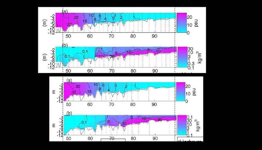
Again, the most important processes are given in bold. Such a second ETM is found for instance
in the Ems River (Fig. 3.2) where high suspended sediment concentrations are found in the fresh
water region, well beyond the head of salinity intrusion. However, Fig. 3.2 suggests that within
the Ems no localized ETM is found, but a large patch of highly turbid water that moves to and
from with the tidal excursion. We anticipate that this is due to the slow remobilization of
sediment from the bed, inducing a longitudinal dispersion of the sediment over the tidal
excursion.
Fig. 3.2: Measured (August 2, 2006) salinity and SPM distributions in the Ems River during flood
and ebb (after Talke et al., 2009) – note that the suspended sediment dynamics have become
independent of the salinity dynamics.
In Section 3.4 we describe qualitatively the evolution from a “normal” estuary to a hyper-
concentrated system, with the Ems River as an example. We argue that it is the change in
dominant processes, e.g. from the balance of equ. (25a) to (25b) which characterizes this regime
shift, and which is responsible for the persistence of this new regime with its second turbidity
maximum (ETM 2).23
3.2 Reduction in effective hydraulic drag
In Chapter 2 we have shown that the response of the tide in a converging estuary is sensitive to
the effective hydraulic drag. In this section we present a simple formula to assess reductions in
hydraulic drag as a function of suspended sediment concentration. Note that these formulae do
not apply for very high concentrations, when fluid mud is formed (occasionally).
Winterwerp et al. (2009) derived a simple formula to quantify the reduction in hydraulic drag as a
function of enhanced levels of suspended sediment concentration and longitudinal salinity
gradients:
u Ceff C C C h
0 SPM 0 4 Ri* (26a)
u* g g g g href
or in terms of excess Chézy coefficient:
Ceff
4hRi* (26b)
g
in which the Rouse number and bulk Richardson number Ri* are defined as:
Ri*
b w gh cgh
and
TWs
u 2
b * w c u*2 u*
(27)
50
40
30
C/g0.5
h= 1m
20
h= 5m
h = 10 m
10 h = 20 m
0
0 0.1 0.2 0.3 0.4
Ri*
Fig. 3.3: Effective hydraulic drag (Chézy coefficient) as function of the bulk Richardson and
Rouse number.
From the implicit equ. (27) we can draw the following conclusions on the effective Chézy
number:
1. The effective Chézy coefficient increases, hence the hydraulic drag decreases with
increasing water depth.24
2. The effective Chézy coefficient increases with suspended sediment concentration c.
3. The effective Chézy coefficient increases with settling velocity, hence with flocculation.
Note that the reduction in effective hydraulic drag is essentially induced by vertical stratification,
induced by vertical gradients in the suspended sediment (SPM) concentration. Because of
hindered settling effects, the same vertical gradient in SPM concentration can exist at relatively
low and relatively high concentrations. Or in other words, low- and high-concentrated mixtures
can be kept in suspension with the same kinetic energy (e.g. Section 3.3).
Hence, the effective Chézy coefficient scales with the following dimensionless parameters:
Ceff
Ri* , (28)
g
The relation between the effective Chézy coefficient and suspended sediment concentrations (e.g.
equ. (26)) is shown in Fig. 3.3. Note that the rivers discussed in this report have water depth of
typically 5 – 10 m, hence we expect an increase in the effective Chézy coefficient by 15 – 30
m1/2/s. Only the Elbe is considerably deeper, and the excess Chézy value is therefore expected to
be larger as well.
3.3 Hyper-concentrated conditions
The literature contains a variety of definitions on hyper-concentrated conditions. In this section,
we present a definition which is relevant for the present study. Winterwerp (2011) argues that the
Ems and Loire River are currently in these hyper-concentrated conditions.
In our definition, hyper-concentrated conditions are related to the concept of saturation (e.g.
Winterwerp, 2001). Let us assume a straight, prismatic channel with a uniform flow at flow
velocity U1. First, we analyze the transport of sand in suspension. From all classical literature,
and data on sand transport, we know that an equilibrium sand transport is established, with an
equilibrium vertical profile in suspended sand concentration, which can be described with a
classical Rouse profile. This profile describes a balance between vertical turbulent mixing and
settling of the grains by gravity. If the flow velocity U1 is reduced to U2, then a new equilibrium
is established immediately, at smaller suspended sand concentrations though. A new equilibrium
between vertical turbulent mixing and settling is established, the suspended sand concentration
being smaller because turbulent mixing is smaller owing to the decrease in flow velocity. Note
that upon deposition from state 1, sand grains form a rigid bed immediately, allowing full
turbulent production, at state 2 conditions, though.
In the case of fine suspended sediment, a different picture emerges, owing to the fact that fine
sediment consists of flocs with high water content (up to 95%). When the flow velocity decreases
from U1 to U2, the fine sediment flocs settle as well, owing to the decrease in turbulent mixing in
response to the lower flow velocity. However, these flocs do not form a rigid bed immediately,
but a layer of soft fluffy sediment. As a result, turbulence production decrease beyond the value
expected at state 2 conditions over a rigid bottom, and more flocs settle, as turbulent mixing drops
further. This snowball effect continues till virtually all flocs have settled on the bed: a layer of
fluid mud has been formed. These conditions are referred to as saturation, and have been
elaborated in detail in Winterwerp (2001).25
A similar condition emerges when the flow velocity is kept constant, but the suspended fine
sediment concentration slowly increases. At a certain level, referred to as the saturation
concentration, vertical turbulent mixing is too small to keep the flocs in suspension, and a fluid
mud layer is formed by the snowball effect described above. This is depicted in Fig. 3.4 (e.g.
Winterwerp, 2011, 2006). The horizontal axis depicts the volumetric concentration of the
suspended sediment, in case of fine sediment, the volume concentration of the flocs; the vertical
axis depicts the flux Richardson number Rif, a parameter describing that part of the kinetic
energy of the flow available for mixing.
super-saturated conditions
low/high-conc. sub-sat. suspension
flux Richardson number Rif
hyper-conc. sub-sat. suspension
U 2 ; U 2 < U1
U1
Ricr
high-conc.
susp.
Ems & Loire conditions
low-conc. susp.
0
0 0.2 0.4 0.6 0.8 1
volumetric concentration f
Fig. 3.4: Stability diagram showing saturation and super-saturated conditions (dotted line). At
smaller concentrations rivers are in the left branch of the diagram, at higher concentrations,
right-branch conditions prevail – these are referred to as hyper-concentrated conditions. The flux
Richardson number Rif yields a proxi for the (kinetic) energy required for vertical mixing, and
this diagram shows that each value of Rif (at sub-critical conditions) can be obtained with two
different volumetric concentrations.
From the above, and from Fig. 3.4 we can conclude that at low suspended sediment
concentrations (left branch of Fig. 3.4), an increase in suspended sediment concentration, for
instance through erosion of the bed, will ultimately lead to a collapse of the concentration profile,
the formation of fluid mud, hence super-saturated conditions. In terms of Fig. 3.4, we follow the
stability curve to the right, and up to larger Rif values until a critical value is surpassed. In
Section 3.2 we have shown that prior to these conditions, already a profound decrease in effective
hydraulic drag may occur.
In the right-hand branch of the stability diagram, we refer to hyper-concentrated conditions. The
suspended sediment concentration is so high, that the sediment’s settling velocity decreases
significantly (up to two orders of magnitude), so that very little turbulent energy/mixing is
required to keep the sediment in suspension. Furthermore, we note that if the flow would erode
sediment from the bed, we would follow the stability curve to the right, but now to lower Rif
values, contrary to the low-concentrated conditions above. This implies that the suspension
becomes more stable: “it likes” to erode the bed, reducing the energy to keep the sediment in
suspension. This is one reason that hyper-concentrated conditions are so persistent, and that
rivers, such as the Ems and the Loire, brought into these hyper-concentrated conditions, are26 difficult to train back into conditions more favorable from an environmental point of view. The reader is referred to Bruens et al. (2012) for a full analysis on the stability of these hyper- concentrated conditions, and why they do not consolidate, but remain fluid over such long periods of time. 3.4 A qualitative description of the regime shift in the Ems estuary Winterwerp (2010) analyzed how the Ems River responded to ongoing deepening. We have no data on the transition of the Ems River from a “normal” turbid river into its current, hyper- concentrated state over time (Fig. 3.2). Therefore, we have developed a conceptual picture for the transition of the river as a result of deepening from its former equilibrium, using our observations described on the previous pages. This picture is summarized in Table 3.1. We start a long time ago from a long-term equilibrium, referred to as phase 0 in Table 3.1, at which up-river directed fine sediment transport induced by gravitational circulation and the various effects of tidal asymmetry balance the down-river transport induced by the river flow. The fine sediments in the Ems River are mainly marine-born, though some sediment may be delivered by the river. Over shorter time periods, accumulation or flushing may occur, as a result of e.g. varying river flows. Under these conditions, the formation of an estuarine turbidity maximum (ETM) is expected near the head of the saline intrusion. Over longer time scales, land formation initiated on vegetated mudflats, may reduce the river’s tidal volume, affecting the long-term morphodynamic equilibrium. As a response to deepening, net accumulation is expected, restoring equilibrium, Phase 1, Table 3.1. The underlying processes are a decrease in river-induced flushing, as river flow velocities decrease in proportion to the river’s cross section, in conjunction with an augmented net transport by gravitational circulation, as water depth increase (scales with h2). Deepening would also increase tidal asymmetry in case of reduced intertidal areas (e.g. Chapter 2). Possibly, reduced vertical mixing already starts to play a role, enhancing the trapping efficiency of the river (see below). As the accumulating fine sediments do not form a rigid bed immediately, also turbidity levels increase, as more sediments are available for remobilization, and suspended sediment concentrations in the ETM increase. A further increase of the river’s depth would increase the amount of remobilizable sediments further, accompanied by a further increase in suspended sediment concentrations. When the riverbed becomes predominantly muddy, profound feed-backs between the various processes are expected through which the river evolves into its present hyper-concentrated state. In this regime, gravitational circulation still plays a role, but its effect is small compared to the dominant contributions of internal tidal asymmetry, with profound differences in vertical mixing during ebb and flood: during ebb, the river is highly stratified by sediment-induced buoyancy destruction. Winterwerp (2010) suggests that this regime shift may be initiated in the Ems River at depth- averaged concentrations typically of the order of a few 100 mg/l. Then, the trapping efficiency of the river increases rapidly as a result of vertical stratification during ebb, and asymmetry in floc size. The rate at which the river really accumulates fine sediments is determined merely by the supply of these sediments from the Wadden Sea – Dollard estuary, than by internal hydro- sedimentological processes. We anticipate a second regime shift in the estuary, Phase 3, Table 3.1, when the river starts to develop pronounced occurrences of fluid mud, as observed presently by Schrottke (2008). In that case, fine sediment transport rates are expected to be dominated by the tidal asymmetry of the
27
peak currents themselves. Now re-entrainment of the fluid mud layers, which scales with U3 as
well, becomes a dominant mechanism (Bruens et al., 2012). Sediment is transported up-river
towards the river’s head at Herbrum by the large tidal asymmetry, and the entire river becomes
highly turbid. As the consolidation rate of fluid mud layers scales with their thickness squared,
we expect that the properties of the fluid mud layer are fully determined by the velocities during
flood conditions. Note that not much consolidation of the thick fluid mud layers during ebb is
expected.
Table 3.1: Summary of Ems River response to its deepening – see text for further explanation;
river depth in Phases 2 and 3 are not necessarily larger than in Phase 1. Phase 0 refers to
“undisturbed” state of the river.
phase dominant transport processes comments
flood-directed transport ebb directed transport
0 “normal” estuary with ETM; equilibrium†) long-term
balance between
(slack water) tidal asymmetry; river-induced flushing
ebb and flood
gravitational circulation)
transport
1 small disturbance; transient state net import;
(slack water) tidal asymmetry ? reduced river-induced flushing weak feed back
enhanced gravitational circ.
2 large disturbance; transient state large net import;
internal tidal asymmetry: mixing & floc size; strong feed-back;
limited sediment load & determined by ebb conditions; large trapping
fairly well-mixed flood; stratified ebb;
relative unimportant grav. circ.; fluid mud;
sediment-induced grav. circ. ? small ebb transport
3 hyper-concentrated estuary; new equilibrium‡) large net import;
asymmetry in tidal velocity; strong feed-back;
internal tidal asymmetry; large trapping
pronounced fluid mud formation;
capacity conditions; transport formula applicable
)
Including possible effects of internal asymmetry, in particular when the salinity field is stratified,
†)
Long-term equilibrium may be disturbed by land formation, reducing estuary’s tidal volume,
‡)
Without maintenance, estuary may return towards its original state if a rigid bed can be formed.
In summary, we infer that in response to deepening of the Ems River, the sediment load in the
river first increases through an increase in the up-river transport by gravitational circulation and a
decrease in river-induced flushing. Then, in the second phase of the river’s transition towards its
hyper-concentrated state, when the concentration in the river attains values of a few 100 mg/l,
internal tidal asymmetry becomes dominant because of pronounced interactions between the
sediment load, and the turbulent water movement and vertical mixing. We believe that the 1990-
survey conditions (e.g. Van Leussen, 1994) fall within this second phase of development. Finally,
the load of fine sediment becomes so large that in the final phase of the river’s evolution, thick
fluid mud layers are formed, and the up-river fine sediment transport is dominated by tidal28 asymmetry of the current velocity. The second phase in transition is probably not stable: trapping is so large that a further development towards the final phase may be inevitable; the time scale of this intermediate phase depends mainly on the sediment supply, and may amount to a decade or so, as in the Ems River. Finally, tidal reflections from the weir at Herbrum are expected to augment the tidal range by a few dm (e.g. Fig. 2.4), further increasing the tidal pumping of mud into the river.
29
4. Comparison of various estuaries
In this section, we compare properties and evolution of a number of estuaries and tidal rivers:
Ems – Germany & The Netherlands
Loire – France
Elbe – Germany
Weser – Germany
Upper Sea Scheldt – Belgium
We have some data available for the Humber (Ouse) and Tamar, both in the UK, the Garonne and
Vilaine, both in France, and the Passaic River in the USA. Note that Kuijper presented similar
analyses for the Western Scheldt estuary.
In the following, the data of the various rivers are analyzed – a synthesis of this analysis is given
in Chapter 5. In this phase of the study we ignore the effects of reflection by a weir, as this is not
easily to be accounted for in an analytical approach. Based on the graphs of Fig. 2.4, it is
anticipated that the tidal amplitude is under-estimated with the single-wave analytical model by a
few decimeter. This implies that a lower friction coefficient (larger Chézy value) is required in
calibrating the model to reproduce observed tidal elevations. However, we expect that the relative
effect of deepening and fine sediments are still reasonably well predicted.
In a next phase of the study we will account for the effects of reflections on barriers/weirs in the
river, but the in current study we discuss the effects of reflections only qualitatively.
The procedure of our data analysis is as follows:
1. We determine the convergence length Lb of the estuary, and its possible variations over
time, by plotting the width of the river against its longitudinal co-ordinate.
2. We establish historical variations in (mean) water depth and intertidal area, and compute
(variations) in the estuarine convergence number e.
3. We compute the imaginary wave number ki between subsequent tidal stations from its
definition a2 a1 exp x2 x1 ki , where a2 = tidal amplitude at x = x2 (etc.), and
make ki dimensionless with Lb.
4. We plot the resulting values of i against e, yielding one data point for each river stretch
in a certain time period.
5. We then fit the analytical model (equ.’s (11)) through the data by tuning the roughness
parameter r*. Note that we assume an infinite long river, but sub-divide the river in sub-
sections with more or less constant water depth.
6. We determine the effective Chézy coefficient C from the fitted r* -values. For this we use
the solution for u from the analytical model (e.g. equ. (41) and (5c)).
7. We plot the variation of C with time identifying possible changes in effective hydraulic
drag over time.
Hence, the linear model discussed in Chapter 2 is merely used as a tool to analyze the historical
data from the various rivers. By making tidal amplification/damping and river
geometry/bathymetry dimensionless, we can compare the various rivers mutually (e.g. Chapter
5).30
4.1 The Ems River
The Ems River is about 53 km long from the weir at Herbrum to Emden, flowing through
Germany into the Ems-Dollard estuary (Fig. 4.1). This river is renowned for its large suspended
sediment concentrations, with values up to 30 – 40 g/l over most of the upper part of the river
(e.g. Talke et al., 2009). These high concentrations are found well beyond the region of salinity
intrusion, and move to and fro with the tide. Also profound layers of fluid mud are found, in
particular around slack water and neap tide (e.g. Schrottke, 2008). Currently, the total mass of
suspended solids amounts to about 1 Mton, while yearly about 1.5 Mton of solids is removed
from the Ems River by dredging. For further details on the river, the reader is referred to Krebs
and Weilbeer (2005).
The Ems River is characterized by a profound tapering, as shown in Fig. 4.2. The overall
convergence length of the river amounts to about 19 km, whereas for the stretches between
Emden – Leeroort Lb ≈ 32 km, Leeroort – Papenburg Lb ≈ 27 km, and Papenburg – Herbrum Lb ≈
33 km. In the following, we refer to these three sections as E-L, L-P and P-H. The apparent
discrepancy of the overall convergence length and those of three smaller stretches of the river is
attributed to some jig-saw patterns in the b-x curve (e.g. Fig. 4.2). In our analysis, we used the
larger values.
Fig. 4.1: Lay-out of Ems-Dollart estuary and Ems River.
An overview of the various interventions in the river was summarized in Vroom et al. (2012),
based on information from Rijkswaterstaat and the Bundesanstalt fur Wasserbau. The evolution
in depths of the river for the three stretches E-L, L-P and P-H is presented in Fig. 4.3, where the
depths have been averaged to obtain mean values for these stretches. Note that after 1940 no
reclamation of intertidal area took place, though we anticipate that a large part of the remainingYou can also read