Mapping Maritime Risk in the Kattegat Using the Automatic Identification System
←
→
Page content transcription
If your browser does not render page correctly, please read the page content below
Mapping Maritime Risk in the Kattegat Using
the Automatic Identification System
Luc van der Lecq

1 March 2021

Thesis for the Degree of Master of Science
MappingMari
          ti
           meRiski
                 nt heKat
                        tegatUs
                              ing
   theAut
        omaticI
              dent
                 ificati
                      onSyst
                           em
                                by

                       L
                       ucv
                         anderL
                              ecq

   1Mar
      ch2021

   Thesi
       sfort
           heDegr eeofMas
                        terofSc
                              ience
   Geographi
           calI
              nformat
                    ionManagementandAppl
                                       i
                                       cat
                                         ions(
                                             GIMA)
   Utr
     echtUniv
            ers
              ity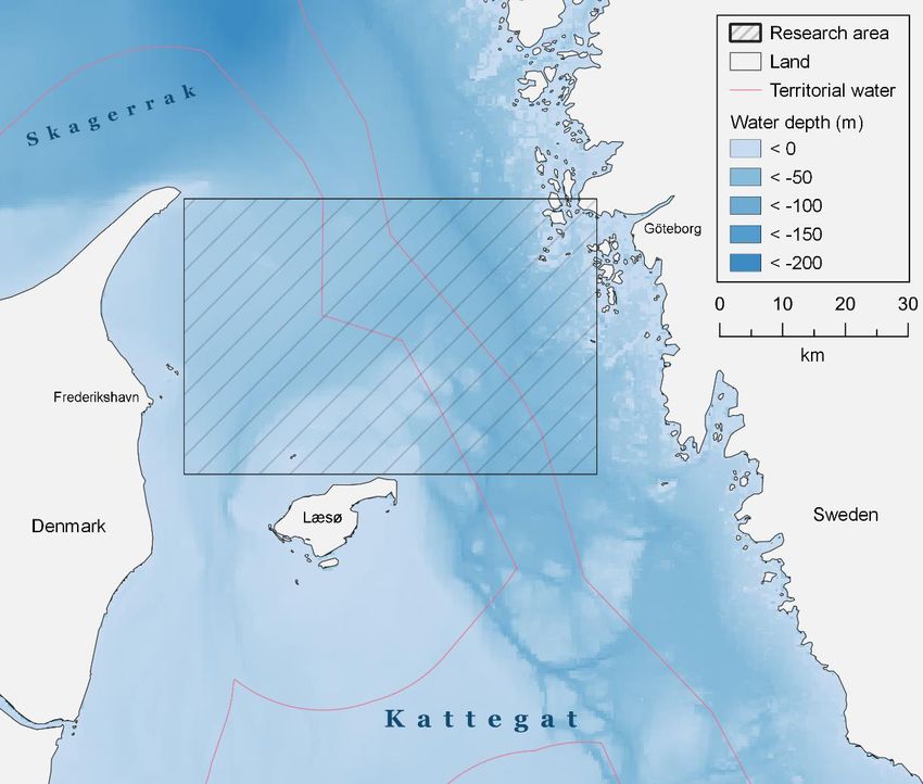
Mapping Maritime Risk in the Kattegat Using the Automatic
Identification System
Thesis for the Degree of Master of Science

Author             Luc van der Lecq
Student number     5719305

Date               1 March 2021

Programme          Geographical Information Management and Applications (GIMA)
                   Faculty of Geosciences
                   Utrecht University (Delft University of Technology, University of
                   Twente, Wageningen University & Research)

Supervision        Martijn Meijers, Delft University of Technology
                   Yigit Can Altan, Delft University of Technology

Responsible        Peter van Oosterom, Delft University of Technology
professor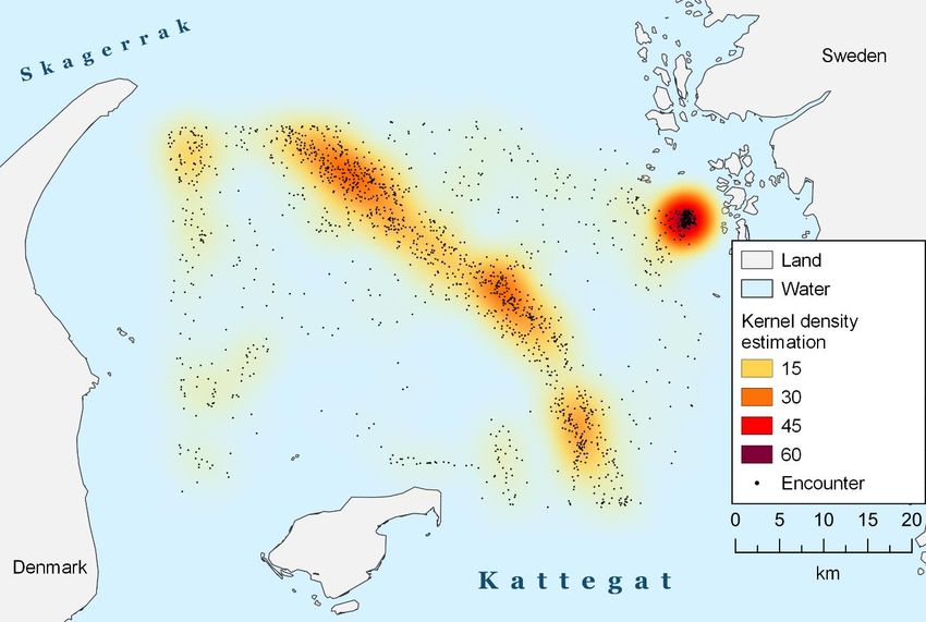
Preface
This thesis on Mapping Maritime Risk in the Kattegat Using the Automatic Identification
System has been written as part of the graduation process of the Geographical Information
Management and Applications (GIMA) Master’s programme, a joint programme between the
universities of Utrecht, Delft, Twente, and Wageningen.

My work on the topic of this thesis started in early July of 2020, partly inspired by my positive
experiences with digital shipping applications at my part time work placement. While initially
aiming to create a comparative case study on the effect of traffic management interventions,
the focus of my thesis work slowly shifted towards exploring the technical details of modelling
vessel movement data and designing a complementary risk analysis system. This balance
proved to be a recurring theme in my research process and keeping it has been an enjoyable
learning experience. Fortunately, my connection with vessel traffic and the Automatic
Identification System does not end with this thesis project, as I will continue my academic
endeavours in the maritime traffic domain in the form of a research internship.

I would like to use this opportunity to thank the people that have helped me complete this
thesis in times of corona. In particular, I have appreciated the helpful comments of and
discussions with my supervisors, Martijn Meijers and Yigit Can Altan. My fellow GIMA
students proved to be indispensable in keeping spirits high, despite the unfortunate closure of
the GIS facilities at Utrecht University. My friends and family also deserve a big thank you for
their valuable feedback and their (online) support on all fronts.

I wish you a pleasant reading experience.

Luc van der Lecq
Utrecht, 1 March 2021

Summary
The Kattegat strait between Denmark and Sweden features high vessel traffic densities and
difficult navigational conditions, making it susceptible to ship collisions. This led to the
implementation of a new shipping route system as of July 2020. This study has assessed the
change in the spatial distribution of maritime risk in the north of the Kattegat after this
implementation and its relation to the spatial pattern of vessel movements and recorded
maritime incidents.
        The maritime risk concept is formed by extracting vessel proximity, encounter type,
speed, and evasive manoeuvres from non-accident critical events. An automated maritime risk
assessment has been developed using vessel tracking data from the Danish Automatic
Identification System (AIS). Several millions of data points have been pre-processed in Python
and stored in a PostGIS database using a basic line segment data model. A three-dimensional
index has been generated to efficiently intersect segments in space and time. A kernel density
estimation has been applied in QGIS to create heatmaps of maritime risk from the detected
vessel encounter locations and their risk values.
        A 17% decrease in encounter frequency has been observed across the entire research
area, which is in line with projections from before the shipping route changes. Maritime risk
values increased slightly. Most ship encounters occurred along the central shipping corridor
from and towards the Baltic sea and involved cargo vessels. This may be because these areas
see the most vessel movements and cargo vessels are the predominant ship type. The maritime
risk pattern along this corridor shifted to the east, which is most likely caused by the shipping
route changes and the corresponding shift in traffic density. Encounters involving passenger
vessels are relatively rare, but have high risk values. This may be due to their crossing of the
busy cargo shipping corridor. It is concluded that maritime risk corresponds to traffic intensity
in terms of the spatial pattern and vessel type. Due to spatial and temporal scope constraints,
the generalisability of this conclusion is limited.
        The result do not show a pronounced relationship between the spatial pattern of
maritime risk and the locations of recorded accidents. Correcting the estimated maritime risk
density for the traffic density bias also did not lead to new insights.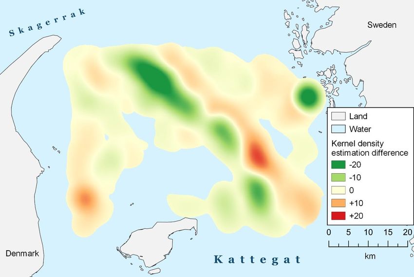
Contents
1     Introduction ............................................................................................................................. 1
    1.1      Problem statement............................................................................................................... 1
      1.1.1         Shipping activity and navigational conditions ...................................................................... 1
      1.1.2         Maritime incidents ..................................................................................................................... 1
      1.1.3         Ship routing changes ................................................................................................................ 2
      1.1.4         Automated maritime risk assessment ..................................................................................... 3
    1.2      Research objectives ............................................................................................................. 3
      1.2.1         Research questions .................................................................................................................... 3
      1.2.2         Spatial and temporal scope ..................................................................................................... 4
    1.3      Research structure ................................................................................................................ 5
2     Theoretical background ......................................................................................................... 6
    2.1      Maritime risk assessment methods ................................................................................... 6
      2.1.1         Maritime risk assessment using recorded accidents ........................................................... 6
      2.1.2         Maritime risk assessment using non-accident critical events ............................................. 6
    2.2      Indicators of maritime risk ................................................................................................... 7
      2.2.1         Ship domain violation ............................................................................................................... 8
      2.2.2         Encounter type ........................................................................................................................... 9
      2.2.3         Speed......................................................................................................................................... 10
      2.2.4         Evasive manoeuvre .................................................................................................................. 10
      2.2.5         Ancillary risk indicators............................................................................................................ 10
    2.3      Database management systems for moving objects ................................................... 10
      2.3.1         Storing spatio-temporal data ................................................................................................. 10
      2.3.2         Indexing and clustering spatio-temporal data .................................................................... 11
    2.4      Knowledge gap .................................................................................................................. 11
3     Methodology ......................................................................................................................... 12
    3.1      The Automatic Identification System .............................................................................. 12
      3.1.1         Principles of the AIS ................................................................................................................. 12
      3.1.2         AIS data from the Danish Maritime Authority ..................................................................... 13
      3.1.3         AIS data from HELCOM .......................................................................................................... 14
    3.2      Vessel traffic analysis .......................................................................................................... 14
    3.3      Maritime risk analysis ......................................................................................................... 15
      3.3.1         Data selection and pre-processing ....................................................................................... 15
      3.3.2         DBMS design ............................................................................................................................ 16
      3.3.3         Vessel trajectory data model .................................................................................................. 17
      3.3.4         Encounter detection ................................................................................................................ 18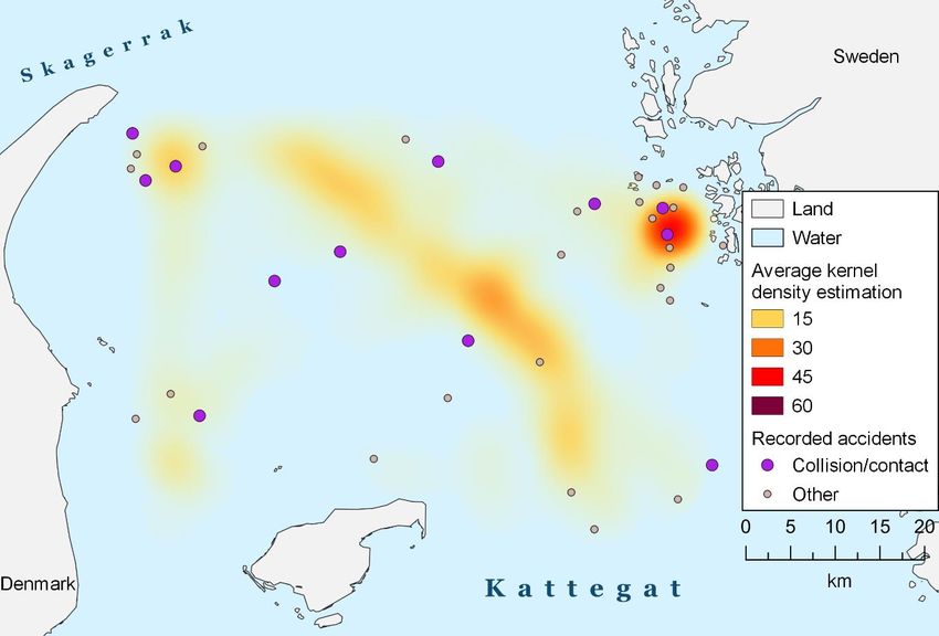
3.3.5          Risk indicator calculation ........................................................................................................ 18
       3.3.6          Heatmap generation ............................................................................................................... 19
       3.3.7          Validation .................................................................................................................................. 20
4      Results .................................................................................................................................... 21
    4.1       Definition and operationalisation of maritime risk ....................................................... 21
    4.2       Spatial pattern of vessel traffic ......................................................................................... 21
    4.3       Spatial patterns of maritime risk ...................................................................................... 23
       4.3.1          Validation .................................................................................................................................. 26
5      Discussion .............................................................................................................................. 28
    5.1       Interpretation of the results .............................................................................................. 28
    5.2       Research limitations ........................................................................................................... 28
       5.2.1          Generalisability of maritime risk results ................................................................................ 28
       5.2.2          Limitations of AIS data ............................................................................................................ 29
       5.2.3          Considerations on modelling and indexing trajectories ................................................... 29
       5.2.4          Improvements to the maritime risk compound .................................................................. 30
6      Conclusion ............................................................................................................................. 31
    6.1       Revisiting the research questions .................................................................................... 31
    6.2       Future work ......................................................................................................................... 32
References ........................................................................................................................................... 33
Appendices ......................................................................................................................................... 36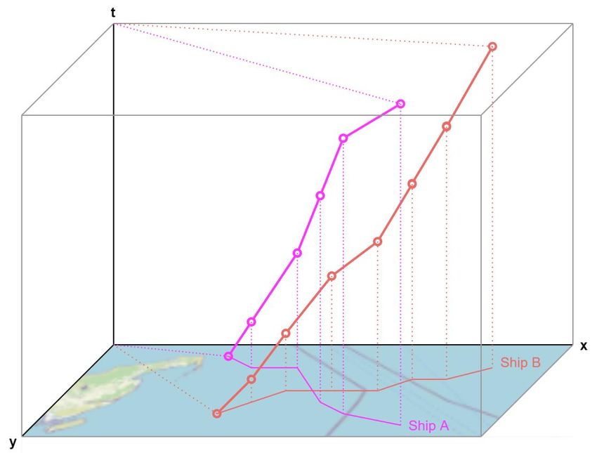
1 Introduction
1.1 Problem statement
With the demand for global transport and seaborne trade showing an upward trend, vessel
traffic intensities across the world’s waterways are high and projected to increase
(International Transport Forum, 2019; Tran & Haasis, 2015). To fulfil this demand efficiently,
vessels are becoming larger and thus require deeper draughts (Tran & Haasis, 2015). Aside
from shipping operations, a wide range of other current developments in the maritime domain
contribute to increasing pressures on the use of sea space. These developments include the
installation of offshore wind farms, the designation of marine protected areas, the exploitation
of mineral resources on the sea floor, and maritime recreation.
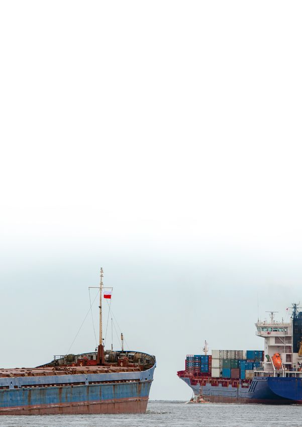
1.1.1 Shipping activity and navigational conditions
The Kattegat strait between Denmark and Sweden is no exception to these global trends and
features heavy international vessel traffic. This strait links the North Sea and the Baltic Sea and
saw nearly 75,000 total ship passages in 2019 (approximately 10,000 unique ships) (Grimvall
& Larsson, 2014). The established shipping routes are primarily used by cargo ships and
tankers (International Maritime Organization [IMO], 2017a). Not only the shipping routes
through the Kattegat see heavier use than those in the Baltic Sea; virtually no part of the
Kattegat area is free of vessel traffic (HELCOM [Baltic Marine Environment Protection
Commission], 2018a). Other relevant groups of vessels are high speed passenger crafts and
ferries crossing the main traffic stream, a large fishing fleet, and smaller, seasonal crafts (IMO,
2017a).
Difficult navigational conditions add a dimension of complexity for ships sailing
through the Kattegat. Large parts of the water between Denmark and Sweden are less than 30
meters deep, limiting the navigable space for deep-draught shipping (Du, Goerlandt, & Kujala,
2020). This results in a relatively high number of groundings (HELCOM, 2018a; IMO, 2017a).
Additionally, the unique environmental configuration of the Kattegat has an impact on
navigational safety. The inflow of salt water from the North Sea versus the inflow of fresh water
from rivers and rain causes spatial differences in water density (Kerbrat, 2018). This can
influence a ship’s draught throughout its passage. The Kattegat is also known for its high
easterly winds in winter and spring, as well as swell from the North Sea (Kerbrat, 2018). Both
of these phenomena result in waves that can impede shipping operations.
1.1.2 Maritime incidents
High vessel traffic densities and difficult navigational conditions make the Kattegat susceptible
to ship collisions (Du et al., 2020). Between 2011 and 2018, a total of 474 maritime casualties
and incidents were reported in the Kattegat region (European Maritime Safety Agency, 2019).
The IMO (2017a) has recorded 20 collisions and groundings between 2000 and 2017. More
than half of the maritime casualties and incidents were caused by navigational issues. The mid-
water phase of a ship’s journey within internal waters or on territorial sea is considered as most
unsafe. No significant decreasing trend in terms of maritime accident events has occurred in
the last decade (EMSA, 2019; HELCOM, 2018a).
Maritime incidents in the Kattegat have a considerable environmental impact. A large
proportion of accidents with pollution (including oil spills) between 2011 and 2016 in the Baltic
Sea occurred along Kattegat shipping routes (HELCOM, 2018b). A valid explanation for this
spatial pattern is given by Lunde Hermansson and Hassellöv (2020): laws and regulations on
1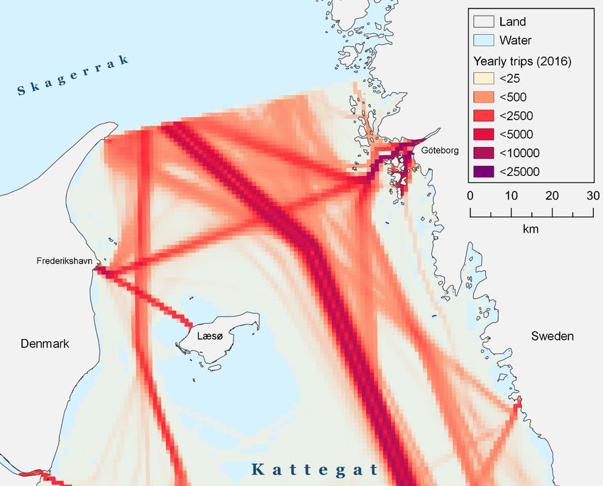
emissions are linked to territorial borders and water depth, resulting in a concentration of tank
washing operations in a small area. Even though the number and size of oil spills shows a
decreasing trend for the Baltic Sea in general, this is not the case for the Kattegat subregion
(reference period 2008-2013) (HELCOM, 2018b).
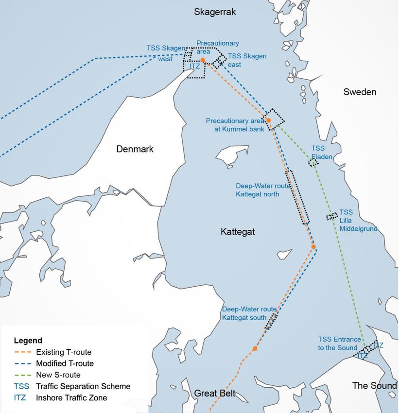
1.1.3 Ship routing changes
In the last ten years, the increase in vessel traffic and number of maritime incidents have
prompted the need for traffic management improvements in the Kattegat. This led to the
development of a new shipping route system (IMO, 2017a). As of July 2020, these changes
have been put in place (Danish Maritime Authority [DMA], 2020). The approved changes
include (1) deep water fairway improvements, (2) alterations in the route to the Great Belt, (3)
a new, shallower route to the Sound, and (4) a number of new traffic separation schemes. A
map of the changes is included in figure 1.1.
Figure 1.1 Ship routing changes in the Kattegat as of July 2020 (SSPA Sweden, 2018)
2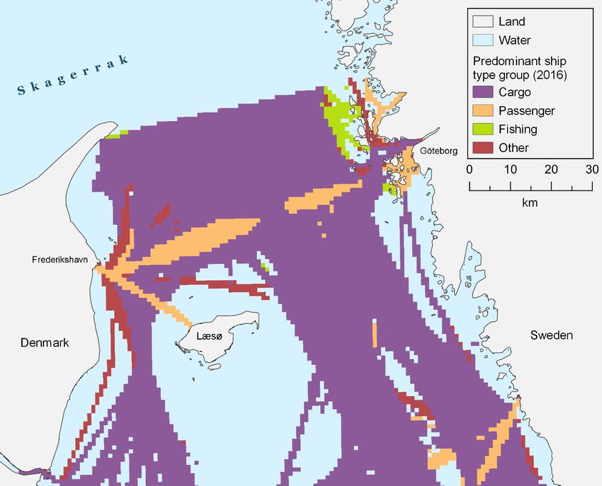
The new situation replaces a 40 year old ship routing system deemed unfit for modern ship
dimensions and traffic separation requirements (IMO, 2017a; Kerbrat, 2018). The goals of
these changes are “to organize the flow of ship traffic in more predictable ways to enhance the
safety of navigation and protection of the marine environment” (IMO, 2017a, p. 1). As the
Baltic Sea handles up to 15 percent of the cargo traffic in the world, achieving these goals is in
the interest of Danish and Swedish authorities and other member states of the IMO (Federal
Maritime and Hydrographic Agency [BSH], 2016).

1.1.4 Automated maritime risk assessment
Manually detecting and analysing the potential risk of maritime incidents in a busy maritime
region like the Kattegat can be labour intensive, imprecise, or disruptive. Using accident
reports proved to be unreliable and the number of reports is too limited for a meaningful
statistical analysis (Du et al., 2020).
         Advancements in data capture and storage technology have paved the way for the
automation of waterway risk assessments. The publication of big digital datasets on vehicular
movements is a particularly relevant development. In this matter, big data relates to both its
volume and velocity (for more detail on the implications of big data for planning transport
systems, see the work of Milne and Watling [2019]). The most notable vehicle tracking dataset
in the maritime domain originates from the Automatic Identification System (AIS).
         The use of vessel encounters extracted from AIS data in lieu of recorded accidents is
common practice in maritime research publications (Du et al., 2020). According to the review
of Du et al. (2020, p. 14), combining a ship domain violation with other risk indicators (e.g.
rate of turn) to detect risky ship encounters is promising. The maritime risk in the Kattegat has
not yet been historically evaluated with this approach. Using this combination can lead to new
insights relating to the automated maritime risk assessment of waterways using large amounts
of vessel movement data.

1.2    Research objectives
The main objective of this research is to identify maritime risk in the Kattegat, with a particular
focus on the differences in risk before and after the ship routing changes of July 2020. Gaining
insight into the changes of risk may have an added value to the operations of maritime
authorities. This main objective requires a definition of risky ship behaviour and its indicators.
Spatial patterns of ship traffic must also be mapped to add context to risky ship encounters.
        The second objective is of a methodological nature and involves the combination of a
ship domain approach with Danish vessel tracking data from the AIS. In order to study
maritime risk using this data source, a scalable database management system (DBMS) must
be designed to manage the large amounts of AIS data. This system should be able to handle
complex queries within reasonable response times. The final DBMS design, as well as the
considerations during its development, may be a valuable addition to the body of knowledge
on database models for movement data.

1.2.1 Research questions
In order to address the problem statement and research objectives, a main research question
is posed:
      To what extent has the spatial distribution of maritime risk changed after the
      implementation of new shipping routes in the Kattegat on 1 July 2020 and how
      does this relate to the spatial pattern of vessel movements and to recorded
      maritime incidents?

                                                                                                      3
Five sub questions serve as building blocks for the main research question. They are:
1. How can maritime risk be defined?
2. How can maritime risk be analysed with spatial movement data?
3. What is the spatial pattern of vessel movements?
4. To what extent has the spatial pattern of maritime risk changed after the
implementation of new shipping routes?
5. To what extent does the spatial pattern of maritime risk relate to the spatial
pattern of vessel movement and recorded maritime incidents?
The sub questions will hereinafter be referred to by their number.
1.2.2 Spatial and temporal scope
Given the spatial extent of the aforementioned ship routing changes, only vessel movements
in a specific part of the Kattegat sea area will be selected to study maritime risk. The northern
limit of this research area is roughly between the Skaw in Denmark and Göteborg in Sweden.
In the west and east, the port areas of Frederikshavn and Göteborg are excluded. The southern
limit of the research area is formed by a line between (1) the Danish town of Sæby, (2) the
Danish island of Læsø, and (3) the start of the new S shipping route towards the Sound. The
total research area covers more than 2,500 km2 and is shown on the map in figure 1.2.
Figure 1.2 Overview of the research area
(Baltic Sea Hydrographic Commission, EuroGeographics, HELCOM)
4No recent changes have been made to the ship routing system in the south of the Kattegat. In
addition, the maritime situation of the Danish straits is not comparable to the spatial
configuration in the north of the Kattegat. For these reasons, the research area definition
excludes vessel movements in the southern part of the Kattegat, the Little Belt, the Great Belt,
and the Sound from the research scope.
The aforementioned ship routing changes in the Kattegat have been effectuated as of 1
July 2020. To evaluate these changes in terms of maritime risk, vessel movement data from a
three month period before 1 July 2020 is selected as a reference period (henceforth referred to
as timeframe 1). This data has been compared to data from 1 July 2020 up to and including
September 2020 (henceforth referred to as timeframe 2).
1.3 Research structure
The flow of this thesis is summarised in figure 1.3. It starts with a comprehensive review of
academic literature. From this theoretical basis, a maritime risk assessment methodology and
a suitable DMBS are developed in tandem. Results are generated using this spatial analysis
method. Finally, the results of the spatial analysis are reflected upon.
Figure 1.3 The flow of the thesis
This flow of reasoning is incorporated into six chapters. Their respective contents are as
follows:
- in chapter 2, existing academic works on maritime risk assessment and database models
for movement data are reviewed;
- next, chapter 3 describes the steps that are required to answer the research questions,
including a motivation for the choices regarding the methodology of this research;
- the main findings are presented in chapter 4;
- chapter 5 provides an interpretation of the results, their meaning in relation to the
theoretical background, as well as the limitations of the research methodology;
- answers to the five sub questions and the main research question are formulated in
chapter 6, as well as directions for future research.
52 Theoretical background
The theoretical background of this research starts with a review of risk assessment methods in
a maritime context in section 2.1. A definition of the constituents of the maritime risk concept
is put forward in section 2.2. This definition contributes towards the answer to sub question 1.
Section 2.3 gives an overview of database models that are suited for storing spatio-temporal
data. A condensed identification of the knowledge gap is presented in the final section of this
chapter.
2.1 Maritime risk assessment methods
The review of Du et al. (2020) identifies a range of methods for studying maritime traffic risk
and safety. Examples include the extraction of maritime movement patterns, anomaly
detection, ship accident probability and consequences modelling, and the statistical analysis
of maritime accidents. A distinction can be made between methods that use non-accident
critical events and methods that have recorded accidents as input.
2.1.1 Maritime risk assessment using recorded accidents
The most direct way of studying maritime risk and safety for a given waterway for a given
period of time is leveraging maritime incident databases and investigation reports. However,
accident reports proved to be unreliable and the number of reports too limited for meaningful
statistical analyses (Du et al., 2020). The underreporting of accident data – which is an
established issue and not limited to the maritime domain – inhibits the use of accident records
for traffic risk assessments, because it may lead to biased risk assessments (Du et al., 2020;
Li, Weng, & Fu, 2020). Selective underreporting may also occur, in the sense that only
incidents of a certain size, impact or at a certain location from the coast (Li et al., 2020). It may
sometimes be in the interest of ship companies to deliberately withhold information during
incident investigations or local procedures may be unclear (Li et al., 2020). An added downside
of accident-based approaches is the lack of contextual information that incident reports
provide (Du et al., 2020).
A statistical analysis of maritime accidents has been performed on the Baltic sea level
(BSH, 2016; Helcom, 2018a). Unfortunately, the cause and location of many recorded
accidents remains unknown or unreported. Accident reports that did include this information
show that collisions are the most common type of accident, especially in the southwestern part
of the Baltic Sea with more than 50%. This percentage has shown an increasing trend in the
last decade. The leading cause of maritime accidents is unintentional human error relating to
navigation. Areas with limited vessel manoeuvrability around ports are main collision hot
spots, as well as the mid-water phase of a ship’s journey within internal waters or on territorial
sea. Construction work at sea and recreational boating in coastal areas are thought to be
complicating factor, as this leads to more potential objects to collide with and more traffic.
2.1.2 Maritime risk assessment using non-accident critical events
Given the drawbacks of using recorded accidents as input for maritime risk assessments, it is
unsurprising that the number of published articles using non-accident critical events has
shown an upward trend between 2006 and 2019 (Du et al., 2020). Non-accident critical events
approaches commonly use vessel tracking information such as AIS as input data. The spatial
tracking of ships allows researchers to evaluate sailing behaviour and other conditions leading
up to an incident. Accident reports may not include this information. Additionally, non-
6accident critical events have a higher occurrence than ship collisions and can be seen as a safety
performance indicator of a maritime traffic system (Du et al., 2020). This has also been found
in practice by Hänninen and Kujala (2014), who report on the relationship between incident
reporting (including near misses) and accident involvement in the Gulf of Finland.
Using non-accident critical events to study maritime risk is based on relational accident
theory. The model structure of this theory can be conceptualised using Hydén’s safety pyramid
(see figure 2.1). It is assumed that several types of events placed on a continuum of severity
occur according to a certain ratio and corresponding frequency (Hydén, 1987). In other words,
ship collisions are thought to seldomly occur and have high impacts, whereas potential
maritime conflicts happen more frequently but tend to have a lower severity or impact. With
this pyramid of proportions in mind, it is only logical that maritime risk assessments rarely
focus on collisions.
Figure 2.1 Conceptual safety pyramid of traffic conflicts
(after Hydén, 1987)
Ship collision risk assessments using non-accident critical events have been performed for
many waterways worldwide. Examples include the coast of Portugal, the North Sea, the
Singapore Strait, the strait of Istanbul, and the Gulf of Finland (Altan & Otay, 2018; Goerlandt,
Montewka, Lammi, & Kujala, 2012; Qu, Meng, & Suyi, 2011; Silveira, Teixeira, & Soares, 2013;
Van Westrenen & Ellerbroek, 2017).
As part of the implementation process of the new shipping routes in the Kattegat (see
section 1.1.3), a commercial analysis of ship collision risk has been performed using data from
the AIS in 2017 (IMO, 2017b). It can be categorised as research on ship accident probability
and consequences modelling. This involved a mathematical model that projects historical AIS
traffic onto a new shipping route layout to create a scenario for comparison. The new
configuration of the shipping routes is expected to lead to a decrease in collisions and
groundings of eight percent (IMO, 2017b). However, this analysis has not been performed with
the exact new shipping route layout that has been implemented. In addition, it does not
consider individual vessel encounters, but uses aggregate data and applies an inflexible
probability factor to calculate maritime risk instead.
2.2 Indicators of maritime risk
A key element of the non-accident critical events approach is classifying events according to
their degree of risk, thereby effectively placing them on the safety pyramid model of figure 2.1.
In a maritime context, this maritime risk concept is formed by (1) modelling ship behaviour
variables extracted from movement data and (2) enriching this data with explanatory
environmental variables. The underlying idea of this model is that situations with a higher
maritime risk have a higher probability of being an accident.
According to Du et al. (2020), the variables speed, course, rate of turn, position,
encounter angle, and ship domain belong to the most used variables to model maritime risk
using non-accident critical events (n=39). These can be grouped into four key factors that
influence maritime risk, which have been conceptualised in figure 2.2. Assessing risky ship
7encounters (i.e. a non-accident critical event) with a ship domain violation is deemed
promising (Du et al., 2020).
Figure 2.2 Conceptual model of key maritime risk indicators
2.2.1 Ship domain violation
A common denominator in research on maritime risk assessments is the definition of a
asymmetrical safety area around a ship that is preferably kept free from other vessels (Du et
al., 2020). This ship domain concept has been introduced in a maritime context in the 1970s
(Fujii & Tanaka, 1971). Ship domains can be the result of theoretical analyses or experts’
knowledge, which tend to be more demanding, heavily parameterised models, whereas more
elementary definitions are generally determined empirically (Szlapczynski & Szlapczynska,
2017). Szlapczynski and Szlapczynska (2017) also note that empirically determined ship
domains may be less suitable for use in the collision avoidance decision making process due to
their relative simplicity. On the other hand, some authors find the complexity of more
advanced ship domain models to be impractical (Szlapczynski & Szlapczynska, 2017).
Regardless of the type of development, the ship domain is commonly affected by the type of
the water region, traffic density, and traffic patterns (Hörteborn, Ringsberg, Svanberg, &
Holm, 2019; Szlapczynski & Szlapczynska, 2017).
Even though the ship domain is one of the most used variables to model maritime risk,
the geometric definition of this domain has considerable variations in the scientific literature
as various authors furthered the work of Fuji and Tanaka between 1970 and 1980 (Du et al.,
2020; Szlapczynski & Szlapczynska, 2017). Early mainstream definitions were established by
Goodwin, Coldwell, and Davis et al. (see figure 2.3). Various authors approach the safety
criterion of the ship domain differently by choosing which domain of the two vessels in an
encounter must be violated by the other’s presence to constitute risk. A more contemporary
approach is that the ship domains of both vessels must overlap for a violation to occur
(Szlapczynski & Szlapczynska, 2017).
Hörteborn et al. (2019) have revisited the debate on ship domain definitions by
analysing its shape using AIS data in the Baltic Sea, including eight locations in the Kattegat
research area of this study. This resulted in a generic ship domain definition of an ellipsoid of
approximately 3.3 by 1.7 kilometres (see figure 2.4). Several additional conclusions were
drawn:
- The ship domain size must decrease in restricted waters.
- The ship domains must attain a more circular shape in a crossing encounter.
- The ship domain is of little significance in a head-on encounter due to the fairway
traffic separation system.
- The ship domain was not dependant on ship size.
8Figure 2.3 Common ship domain definitions (A: Goodwin, B: Coldwell, C: Davis and co.)
(adopted from Theunissen & De Groot, 2014)
Figure 2.4 Empirically determined generic ship domain definition for the Baltic Sea
(after Hörteborn et al., 2019)
2.2.2 Encounter type
The encounter angle is identified as a key indicator for modelling maritime risk (Du et al.,
2020). The encounter situation of two vessels can be divided into three subgroups using this
variable. When considering the individual trajectories of two vessels during an encounter, the
encounter type is deducted from the encounter angle (defined as the difference between the
course over ground, ΔCOG) between the two vessel. These three subgroups are generalised as:
- Head-on encounter
|ΔCOG| = 180° with a given offset
- Overtaking encounter
|ΔCOG| = 0° with a given offset
- Crossing encounter
0° < |ΔCOG| < 180 with a given offset or 180° < |ΔCOG| < 360 with a given offset
92.2.3 Speed
The speed difference variable is identified as a key indicator for modelling maritime risk (Du
et al., 2020). When considering the individual trajectories of two vessels during an encounter,
the speed difference is defined as the difference between the speed over ground (ΔSOG)
between the two vessels. The speed difference variable has a positive relation with the maritime
risk compound.
2.2.4 Evasive manoeuvre
Evasive manoeuvres during vessel encounters may indicate risky shipping behaviour. Such an
evasive manoeuvre can be detected by assessing the rate of turn level of a vessel during its
journey, because a high rate of turn level is a rare occurrence during normal shipping
operations and may results from last moment evasive action (Mestl, Tallakstad, & Castberg,
2016). This rate of turn (ROT) variable is commonly used as a key indicator for modelling
maritime risk, as “it is straight forward and indeed very fast to single out potential critical
situations characterized by non‐normal manoeuvres” (Du et al., 2020; Mestl et al., 2016, p.
76).
Mestl et al. (2016) note that high rate of turn levels in themselves are not sufficient
indicators and propose a method of combining the turning rate with vessel speed to more
accurately reflect abnormal shipping behaviour. The product of the ROT and SOG variables
allows for the calculation of the centripetal acceleration (CA) of a vessel, which is defined as
the change in rotation around the vertical axis to which people on a ship are exposed. The
centripetal acceleration variable has a positive relation with the maritime risk compound.
2.2.5 Ancillary risk indicators
A range of additional factors can be identified that lie outside the vessel tracking information
domain. The following groups of ancillary risk indicators are not included in the conceptual
model of figure 2.2, as they are considered to lie outside of the scope of this research. They are,
however, indicators of maritime risk.
Firstly, external causes affect safe shipping operations (BSH, 2016; Helcom, 2018a).
Examples includes adverse weather, poor visibility, and strong currents (Shu, Daamen,
Ligeringen, & Hoogendoorn, 2013). Second, technical equipment failure is a considerable
contributing factor in shipping accidents (BSH, 2016; Helcom, 2018a). An example of this is
machinery failure. Thirdly, some psychological and social elements of human error behaviour
cannot be deducted from vessel tracking information such as AIS data. A key example is the
decreased vigilance of mariners on the bridge.
2.3 Database management systems for moving objects
2.3.1 Storing spatio-temporal data
Given the increasing availability and magnitude of data from vessel tracking systems, finding
a suitable data model and implementing it in a database system to store and analyse spatio-
temporal data is challenging. Classical spatial database management systems can handle
moving objects, but cannot handle time intrinsically. GIS functionality for analysing moving
objects is therefore limited, as support for handling temporal information has not entered the
mainstream (Graser, 2018).
The current state of the art of open source technology with temporal support has been
identified in the work of Graser and Dragaschnig (2020). Two groups of tools and software
come to the fore: desktop GIS and spatial databases, interactive notebook environments, and
distributed computing solutions. A typology of these two groups is given in table 2.1.
10Table 2.1 Typology of current GI technology with support for temporal information
(after Graser & Dragaschnig, 2020)
Technology groups Software and tools Features and characteristics
Easy interactive mapping
QGIS, PostGIS, Built-in trajectory functions
Desktop GIS and spatial databases
Jupyter, MovingPandas Less suited for big datasets
Lower hardware requirements
Limited trajectory functionality
GeoMesa, M³, SPARK, Dedicated spatio-temporal indexing
Distributed computing solutions
MobilityDB Designed for big datasets
Advanced hardware requirements
With growing amounts of data demanding more processing power, recent scientific efforts
have been focused on the development of distributed big data computing tools (see the work
of Graser, Widhalm, and Dragaschnig [2020] and Bakli, Sakr, and Zimanyi [2020] for novel
applications). Even though desktop GIS, spatial databases, and interactive notebook
environments are primarily used on a single computer, recent developments have paved the
way for parallelisation of these tools, too (Graser, 2018; Graser & Dragaschnig, 2020).
2.3.2 Indexing and clustering spatio-temporal data
The aim of database management systems for moving objects is to introduce the possibility of
representing and querying moving objects to existing database technology. Spatial databases
allow for efficient querying of stationary two dimensional objects by creating a hierarchical tree
using the bounding boxes of the spatial features, which can then be traversed to find objects.
This index is stored separately and reduces the duration of a database scan during a query.
Accommodating moving objects is more difficult (Güting et al., 2000). Many researcher
have worked on indexing spatio-temporal objects (Graser, 2018). In the context of vessel
tracking information systems like the AIS, a given set of spatio-temporal objects can be
considered as having a third dimension, namely time. Following from this, indexes aimed at
moving vessels may apply a three dimensional bounding box to efficiently access the data of
parts of a vessel’s trajectory in three dimensional space (Graser, 2018).
The performance of database management systems depends on the data retrieval speed
from the physical disk, especially for large databases that transcend the storage capacity of the
RAM (Van Oosterom, 2005). Decreasing this speed may be achieved by implementing a
clustered index. A clustered index not only stores a hierarchical tree containing the order of
objects, but also rearranges the data on the physical disk accordingly. For a spatial database,
this means that proximate objects are stored in the same physical data block.
2.4 Knowledge gap
The introduction in the first chapter of this research documentation and the previous sections
in this literature have led to the following unexplored scientific opportunities:
- The combination of non-accident critical events approach with key maritime risk
indicators including a ship domain violation in the Kattegat is a unique approach in the
body of literature on maritime risk assessments.
- Using a relatively accessible data model to represent ship trajectories in a PostGIS
DBMS may add to best practices in the movement data science domain.
- The work of Du et al. (2020) reveals that approximately 20 percent of the selected
published articles validated their model using a reality check. This leads to a need for
scientific evidence that validates already existing research approaches, as opposed to
proposing new methods for maritime risk assessments (Du et al., 2020).
113 Methodology
The methodological procedure of this research project is divided into three main sections. The
first section contains information on the most important data source of this research project,
namely the Automatic Identification System. Section 3.2 describes the workflow of analysing
vessel traffic patterns in the research area. The third section on the maritime risk analysis is
the largest and first discusses the design of a suitable DBMS for large amounts of spatial
movement data. It also elaborates on data pre-processing steps, mapping encounter risk, and
validating detected encounters.
3.1 The Automatic Identification System
The Automatic Identification System (AIS) exchanges navigational and voyage related
information between ships and shore stations via very high frequency radio (VHF) (Harati-
Mokhtari, Wall, Brookes, & Wang, 2007). In its essence, the AIS is a form of remote sensing
according to a Lagrangian frame of reference, because it entails the continuous tracking of
object (Dodge, Weibel, Ahearn, Buchin, & Miller, 2016). The promise of the AIS is an enhanced
level of safety and efficient navigation at sea, because mariners receive continuous and
automatic updates on ship movements in their surroundings. This applies especially to areas
where more traditional navigational aids such as radar fall short. Examples are detecting ships
around bends or behind landmasses. The AIS also poses benefits for maritime environmental
protection, situational awareness, and waterway management (DMA, n.d.). These objectives
and circumstances of use are in line with the current maritime situation of the Kattegat (see
section 1.1). For this reason, vessel information from the AIS is a suitable starting point for a
maritime risk analysis of the Kattegat sea area.
3.1.1 Principles of the AIS
In its core, the AIS is made up of ship-born transceivers and land based transceivers (see figure
3.1). The transceivers broadcast AIS messages regularly and automatically. The information
that is received can be visualised and used for navigational decision making. This information
can contain three types of content (IMO, 2015):
- Static information
This type of information is used to identify a vessel, its type, and to describe its
physical dimensions.
- Dynamic information
This type of information covers the vessel location and the corresponding timestamp,
as well as other navigational readings from vessel instruments.
- Voyage information
This type of information relates to the cargo of a vessel and its destination, which are
to be manually entered for each voyage.
The IMO (2015) distinguishes two shipborne equipment classes, with each class having
different technical specifications and intended applications. Class A equipment is required for
all vessels of more than 300 gross tonnage on international voyages, cargo vessels of more than
500 gross tonnage not on international voyages, passenger ships of all sizes, and fishing vessels
longer than 15 metres. This type of equipment is highly advanced, more expensive, and aimed
at commercial use. The reporting interval of class A units ranges from a maximum of 180
12seconds when the vessel is at anchor or moored and not moving faster than 3 knots, to a
minimum of 2 seconds when moving faster than 14 knots and changing course.
Class B transceivers may be installed on vessels that are not bound by class A
regulations. These transceivers are generally less advanced, less costly, and aimed at lighter
commercial vessels and smaller, seasonal crafts. In general, class B units have a lower reporting
frequency, with the transmitting interval ranging from 180 to 30 seconds.
Figure 3.1 Overview of the AIS
(after IMO, 2015)
3.1.2 AIS data from the Danish Maritime Authority
The Danish Maritime Authority (n.d.) captures, processes, and publishes AIS data of vessel
traffic in Danish waters and their surroundings. It is made publicly available on the basis of
the Directive on the re-use of public sector information (PSI Directive) of the European Union.
The historical data is published in a text file format with a delay of approximately three days.
Figure 3.2 gives an indication of the magnitude of the data files, with each text file containing
millions of data points. A small sample of data points from a single text file is included in
appendix A.
The key elements of the Danish AIS data are a timestamp and coordinates, thereby
making it spatio-temporal object information. Additional relevant elements of the Danish
dataset include vessel characteristics (e.g. identification, vessel type, dimensions, cargo type)
and navigational indicators from vessel sensors (e.g. speed, heading, course, rate of turn). The
majority of data points in this dataset originate from class A equipment, but it also includes
reports from class B units.
Figure 3.2 File size of AIS text files published by the DMA for timeframe 1 and timeframe 2
133.1.3 AIS data from HELCOM
HELCOM publishes shipping density raster files in the GeoTIFF format for all ships with AIS
equipment, as well as separate raster files that only include data from various ship types. These
raster files are publicly available without limitations, with attribution being the only
requirement for reuse (HELCOM, 2018c). The HELCOM AIS system is fed by national data
from Baltic Sea States, including data from Danish sources. Its spatial scope is limited to the
Baltic sea. It includes the Kattegat and excludes the Skagerrak.
The shipping density raster files were created by HELCOM according to the following
workflow (see HELCOM [2018c] for details). First, a total of 339 port entrance areas were
established across the Baltic Sea States, as well as 5 areas representing the Baltic Sea borders.
Secondly, AIS point data from the HELCOM AIS system were transformed into lines, ensuring
that each line represents a unique ship movement between two ports, from an inbound
crossing of the Baltic Sea borders, or towards an outbound crossing of the Baltic Sea borders.
Finally, the resulting lines were overlaid on a 1 x 1 km grid where for each raster cell the number
of trips crossing it was calculated and stored.
3.2 Vessel traffic analysis
The vessel traffic analysis is aimed at providing context for the subsequent main analysis of
maritime risk. Results from this analysis form the basis of the answer to sub question 3.
The workflow of this analysis is shown in figure 3.3. The first step of this procedure was
taking the shipping density raster files of nine ship types from HELCOM and clipping them to
the Kattegat area. The resulting raster files were locally aggregated according to the grouping
in table 3.1, resulting in four raster layers representing a distinct ship type (cargo, passenger,
fishing, and other ships). Finally, the ship category with the highest intensity value was selected
for each individual cell in order to create a predominant ship type raster map.
This final step of this analysis has been performed using the ArgStatistics algorithm in
Esri’s ArcGIS Pro, because this implementation of a local maximum operation was not readily
available in other common GIS software.
Figure 3.3 Methodological steps of the vessel traffic analysis
Table 3.1 Aggregation of ship types from HELCOM raster files into four distinct groups
Cargo Passenger Fishing Other
cargo passenger fishing other
container service
roll-on/roll-off unknown
tanker
143.3 Maritime risk analysis
The maritime risk analysis is the main methodological process of this research and consists of
both exploratory and confirmatory data analyses. Figure 3.4 gives a schematic overview of the
maritime risk analysis. The development of this methodology contributes to answering sub
question 2, while the results of this analysis contribute towards the answer to sub question 4.
The first step involved importing AIS data into a PostGIS DBMS that suits the
functional requirements of subsequent spatial analyses. A process of data preparation in the
database was performed to control data quality. Subsequently, the original point locations were
transformed into a line segment model. The analysis continued with a main phase of analysis
aimed at discovering spatial patterns of maritime risk. The procedure to create maps from AIS
text files was identical for both timeframes 1 and 2. The final methodological steps included
comparative mapping and the validation of results.
Figure 3.4 Methodological steps of the maritime risk analysis
3.3.1 Data selection and pre-processing
The first part of the maritime risk analysis involved importing AIS data into a PostgreSQL
database with the PostGIS extension. Due to the limitations of consumer grade computer
equipment in terms of data storage and processing power, a subsample of the available data
was analysed. Only the text files of a random sample of 15 days per timeframe were selected
(see table 3.2). From this selection of 40 files, only vessel movements within the research area
(see figure 1.2) were analysed to reduce complexity. The data pre-processing procedure of
reducing the number of data points has been scripted in Python using the pandas library. It
includes attribute filters and a bounding box filter (see appendix B for scripts).
15Table 3.2 Random sample of 15 days from timeframes 1 and 2 for text file data import
Timeframe 1 Timeframe 2
2020-04-08 2020-05-05 2020-06-06 2020-07-01 2020-08-07 2020-09-05
2020-04-12 2020-05-16 2020-06-09 2020-07-03 2020-08-16 2020-09-06
2020-04-18 2020-05-24 2020-06-12 2020-07-04 2020-08-21 2020-09-13
2020-04-22 2020-05-29 2020-06-16 2020-07-17 2020-09-18
2020-04-27 2020-06-17 2020-07-18 2020-09-21
2020-04-30 2020-07-30 2020-09-29
A lack of data accuracy and consistency can be expected in AIS datasets (Felski & Jaskólski,
2012; Harati-Mokhtari et al., 2007; Zhao et al., 2018). Controlling this quality was crucial
throughout the maritime risk analysis, as the accuracy of navigational indicators had a
considerable influence on the detection of vessel encounters. As mentioned in section 3.1.1, AIS
specifications generally stipulate that at least one message must be sent every 75 meters or 180
seconds approximately. The system achieves this by making the reporting interval dependant
on speed. For this reason, line segments in the DBMS that greatly exceed these limits were
deemed invalid during the data cleaning process and have been left out (see appendix B for the
corresponding query).
3.3.2 DBMS design
A database design of four tables has been established in the PostGIS DBMS to store the various
intermediate products of the maritime risk analysis. Figure 3.5 gives a schematic overview of
this design. The points table was filled with the results of data pre-processing procedure. The
segments table contained a similar number of data points as the points table, because each
segment consists of a start and end point. The encounter_segments table is made up of a subset
of this number of rows, as only a relatively small portion of all vessel segments represent
encounter situations. This detection process, as well as the grouping of encounter segments
into higher level unique encounters is discussed in section 3.3.4.
Figure 3.5 Table configuration and general flow of information of the PostGIS DBMS
163.3.3 Vessel trajectory data model
Over the course of this thesis project, four types of data models were considered to approximate
a ship’s trajectory based on AIS data from the DMA in a PostGIS database. They were:
- a 2D Point model
A two dimensional points representation (x,y) with a timestamp attribute;
- a basic 2D line segment model
A line representation, consisting of a maximum of two two-dimensional points (x,y)
with a start timestamp attribute and end timestamp attribute;
- a basic 3D line segment model
A line representation, consisting of a maximum of two three-dimensional points
(x,y,t);
- a full trajectory 3D line model
A LinestringM representation, consisting of multiple three dimensional points (x,y,t).
The choice was made to transform the discrete ship position points into a basic 3D line segment
data model. The PostGIS query for this step is included in appendix B. Together, these line
segments make up the full trajectory of a vessel’s journey, as visualised in figure 3.6.
A line segment model has benefits over a point-based model, especially when the
historical AIS data has been stored at irregular intervals (Graser, 2018). This is because a series
of line segments has a more continuous nature than a series of points. The basic 3D line
segment model was also beneficial for the efficiency of the DBMS during analyses, because
choosing short lines as opposed to a full trajectory LinestringM data model made it possible to
use multidimensional indices (see also section 2.3.2) (Graser, 2018). The implementation of
the full trajectory line model has only recently been added to the PostGIS toolbox. It is
therefore assumed that using the core functionality associated with the basic line
representation benefits from better support in terms of its implementation and its use in other
PostGIS functions.
Figure 3.6 Illustrative representation of ship trajectories using the basic 3D line segment model
173.3.4 Encounter detection
The methodological process of this research project continues with the main phase of spatial
analysis (light grey in figure 3.4). The steps that are involved with the encounter detection and
risk indicator calculation are shown in figure 3.7. The PostGIS queries that correspond to these
steps are included in appendix B.
The line segments of the vessel trajectories were the starting point of this phase of
analysis. First, a three-dimensional index was created on the geometry of the line segments.
This allowed for intersecting large amounts of line segments considering space and time in an
efficient way (see section 2.3.2). All ship pairs that were within approximately 1,000 meter of
each other and occurred at an overlapping time interval were stored in the
encounter_segments table in order to guarantee the ship domains of two vessels to overlap. As
an encounter of two vessels can take place over a prolonged period of time, the encounter
segments were grouped based on ship identification numbers and time of the encounter.
Finally, these groups were dissolved and stored as unique higher level encounters in the
encounters table.
Figure 3.7 Methodological steps of the encounter detection and risk indicator calculation
3.3.5 Risk indicator calculation
A total of five risk indicators were calculated that moderate the maritime risk value of each
higher level encounters in the encounters table,. This process is shown in the lower grey box in
figure 3.7. The five indicators that were used in this study are based on the maritime risk factors
from section 2.2.
18You can also read