Social Network Analysis with Content and Graphs
←
→
Page content transcription
If your browser does not render page correctly, please read the page content below
SOCIAL NETWORK ANALYSIS WITH CONTENT AND GRAPHS
Social Network Analysis
with Content and Graphs
William M. Campbell, Charlie K. Dagli, and Clifford J. Weinstein
Social network analysis has undergone a
renaissance with the ubiquity and quantity of
» As a consequence of changing economic
and social realities, the increased availability
of large-scale, real-world sociographic data
content from social media, web pages, and
has ushered in a new era of research and
sensors. This content is a rich data source for development in social network analysis. The quantity of
constructing and analyzing social networks, but content-based data created every day by traditional and
social media, sensors, and mobile devices provides great
its enormity and unstructured nature also present
opportunities and unique challenges for the automatic
multiple challenges. Work at Lincoln Laboratory analysis, prediction, and summarization in the era of what
is addressing the problems in constructing has been dubbed “Big Data.” Lincoln Laboratory has been
networks from unstructured data, analyzing the investigating approaches for computational social network
analysis that focus on three areas: constructing social net-
community structure of a network, and inferring
works, analyzing the structure and dynamics of a com-
information from networks. Graph analytics munity, and developing inferences from social networks.
have proven to be valuable tools in solving these Network construction from general, real-world data
presents several unexpected challenges owing to the data
challenges. Through the use of these tools,
domains themselves, e.g., information extraction and pre-
Laboratory researchers have achieved promising processing, and to the data structures used for knowledge
results on real-world data. A sampling of these representation and storage. The Laboratory has devel-
results are presented in this article. oped methods for constructing networks from varied,
unstructured sources such as text, social media, and real-
ity mining of datasets.
A fundamental tool in social network analysis that
underpins many higher-level analytics is community detec-
tion. Various approaches have been employed to detect
community structure from network data, including a tech-
nique to explore the dynamics of these communities once
they are detected. Insight gained from basic analytical tech-
niques, such as community analysis, can be used for higher-
level inference and knowledge-discovery tasks. Work in
attribute prediction on social networks takes advantage of
recent advances in statistical relational learning.
62 LINCOLN LABORATORY JOURNAL VOLUME 20, NUMBER 1, 2013
WILLIAM M. CAMPBELL, CHARLIE K. DAGLI, AND CLIFFORD J. WEINSTEIN
Graph Construction individuals (e.g., bank accounts, Paypal), collaboration
Social networks are embedded in many sources of data or references (e.g., patent, research, movie databases),
and at many different scales. Social networks can arise and human-annotated and -entered data. The research
from information in sources such as text, databases, sen- described in this article used a database collected by the
sor networks, communication systems, and social media. Institute for the Study of Violent Groups (ISVG) [10]. This
Finding and representing a social network from a data database contains people, organizations, and events anno-
source can be a difficult problem. This challenge is due tated and categorized into a standard Structured Query
to many factors, including the ambiguity of human lan- Language (SQL) relational database structure [5].In addi-
guage, multiple aliases for the same user, incompatible tion, a database of sensor data from the reality mining cor-
representations of information, and the ambiguity of rela- pus [1] is used for dynamic social network analysis.
tionships between individuals.
INFORMATION EXTRACTION FROM TEXT
Data Sources and Information Extraction Information extraction (IE) is a standard term in human
Two primary open sources of social network information are language technology that describes technology that auto-
newswire and social media. Various research efforts examine matically extracts structured information from text [11].
other sources of social network data—smart phones [1–3], A popular subarea in IE is named-entity recognition
proximity sensors [4], simulated data [5, 6], surveys, com- (NER). NER extracts people, places, and organizations
munication networks, private company data [7], covert or that are mentioned in text by proper name (as opposed
dark networks, social science research, and databases. to being referenced by pronominal terms, e.g., “you,” or
Text information from newswire provides informa- nominal forms, e.g., “the man”).
tion about entities (people and organizations) and their Constructing social networks from text can be accom-
corresponding relations and involvement in events [5]. plished in several ways. An overall description of the pro-
This information is encoded in text in multiple languages cess is shown in Figure 1. The simplest approach is to use
and numerous formats. Extracting entities and their rela- links based upon the co-occurrence of entities in a docu-
tions from newswire stories is a difficult task. ment. This approach can be accomplished with simple
Sensors can also serve as sources of data for social string matches [8] or with full-scale NER [5]. This co-
networks [2]. Smartphones and proximity devices [4] occurrence approach works reasonably well with certain
can provide information about dynamic interactions in genres of documents (e.g., newswire reports) in which
social networks and can aid in the corresponding analysis two entities mentioned together are presumed likely to
of those networks. Predicting behavior, personality, iden- be related. This approach fails for long documents that
tity, pattern of life, and the outcome of negotiations are cover a wide range of topics (e.g., a survey report). For the
a few of the proposed applications that may exploit data latter case, the co-occurrence approach can be refined to
from sensor systems. narrower parameters, such as “occurs in the same para-
Communications and social media have been ana- graph, sentence, or even subject topic” of a given report.
lyzed for social network structure. For example, the A second approach to extracting networks is to look
release of the e-mail related to Enron’s bankruptcy, and for mentions of relationships in text [11]. For instance, in
subsequent prosecution for fraudulent accounting prac- a document, Bob and Mary are referred to as brother and
tices [8], has provided a limited window into company sister. This approach is compelling but has drawbacks. In
dynamics and e-mail flow. In the case of social media, an many situations, relationships are implicit and not stated.
analysis of followers in Twitter shows networks of users The problem then becomes a process of inferring relations
who are related by current news topics rather than by from text. Even with human annotators, making such
personal interactions [9]. Other social media companies inferences is a difficult task with high inter-annotator
such as Facebook may also provide network data sources, disagreement for some tasks [11].
although privacy is a major concern. A final issue in the extraction of entities from text
Databases can provide networks in structured form. is that of co-reference resolution. The problem arises
Examples of database types include transactions between because mentions of a name within and across documents
VOLUME 20, NUMBER 1, 2013 LINCOLN LABORATORY JOURNAL 63
SOCIAL NETWORK ANALYSIS WITH CONTENT AND GRAPHS
Source document collection text, speech, image), analysts produce a set of objects,
attributes, and predicates conforming to an ontology
that describes structured information in the document.
An ontology based on standards for information extrac-
tion, primarily the Automated Content Extraction (ACE)
protocol [11], is common.
A typical example extraction from a document might
Named-entity detection be Member (Bob, KarateClub) where Bob is an object of
& within-document co-reference
resolution type per (a person) and KarateClub is an object of type
organization. The statement Member (·,·) is a predicate
and describes some relation between the entities.
An important point is that representation is usually
limited to binary predicates, i.e., relationships of the form
Cross-document Relation (entity, entity). At first, this might appear to be a
co-reference resolution
constraint. For instance, how does one represent multiple
entities participating in a meeting or event? The key is
to create a meeting entity, M, and then state all relations
Link analysis between all people, P, involved in the meeting and M, e.g.,
Participates (Bob, M), Participates (Fred, M), and so on.
FIGURE 1. Information extraction from a corpus of docu- Another property is that objects can have attributes.
ments for social network construction is accomplished by For instance, it is possible to extract ATT_age (Bob, 25).
first performing named-entity detection and co-reference Attributes can be complex. For instance, one attribute of
resolution within a document followed by co-reference resolu- Bob could be the text document of his resume.
tion between documents. Networks can then be constructed
The knowledge representation approach is equivalent
using links of different types found between the entities.
to a relational database model. In fact, the original work
on relational databases by Codd [14] used a predicate
vary—John, John Smith, Mr. Smith. Co-reference resolu- model and corresponding “calculus” for manipulation.
tion combines all of these variants into one entity. How- Each predicate corresponds to a table, and the entities in
ever, a quick look at “John Smith” on Wikipedia shows the relations are stored in the table. A typical example is
that a name alone is not sufficient to disambiguate an shown in Figure 2.
entity. Co-reference resolution is difficult within docu- Note that because our relations are binary, an alter-
ments, and across-document resolution is even harder. nate database structure is a triple store, which is designed
to store and retrieve identities constructed from a set of
Representation three relationships. The triple in this case is (predicate,
Once a social network is extracted from the original data val1, val2). Triple stores have become popular lately in
source, it must be stored in structured form so that auto- the Resource Description Framework (RDF) used by the
matic analysis, retrieval, and manipulation are possible. World Wide Web consortium for the Semantic Web [15].
Multiple possible structures for the representation are
mathematically equivalent. The main difference among ATTRIBUTED GRAPHS
them is that they arise in multiple fields. Two such rep- An alternate representation of social network data is to
resentations are knowledge representation and graphs. view the knowledge representation structure as a graph.
The knowledge representation approach lends itself
KNOWLEDGE REPRESENTATION naturally to graph “conversion.” Figure 3 shows the basic
Extracted structured content from raw data can be process through a restructuring of the data in Figure 2
encoded using standard knowledge representation meth- as a graph. The basic process is as follows. Entities are
ods and ontologies [12, 13]. For every input datum (e.g., converted to nodes in the graph. Note that the nodes
64 LINCOLN LABORATORY JOURNAL VOLUME 20, NUMBER 1, 2013
WILLIAM M. CAMPBELL, CHARLIE K. DAGLI, AND CLIFFORD J. WEINSTEIN
Knows Age: 25 Age: 67
Bob John Knows
ATT_Age Bob John
Bob Fred
Bob 25
John Tom Knows Knows
Fred 35
... ...
John 67
Fred Tom
... ...
Age: 35
FIGURE 2. Knowledge representation in a relational data- FIGURE 3. The directed edges of this attributed graph
base. Standard knowledge representation schemes usually example show the unidirectional Knows relationship
involve binary predicates defining relationships between between Bob and both John and Fred, and the unidirectional
entities. This knowledge representation approach is equiva- relationship between John and Tom. This view of knowledge
lent to a relational database model as shown above for the representation lends itself more easily to graph analysis
predicates, Knows and ATT_Age. problems and approaches.
can have different types—e.g., people, organizations, and in real social networks. For the purposes of this article,
events. This model deviates from the standard model of assume that the communities are disjoint, that is, member-
a graph in which the node set is one type. Edges in the ship in one community precludes membership in another.
graph correspond to relations between entities, so the In considering the problem of community detec-
relation Knows(Bob, Fred) is converted to a directed edge tion for social networks, Lincoln Laboratory researchers
between nodes with the Knows attribute. Note that if we applied multiple algorithms in the literature to the prob-
wanted a relation to be bidirectional [Knows(a , b) implies lem of community detection on the ISVG database. The
Knows(b , a)], an undirected edge could be used between goal was to partition a set of people into distinct violent
nodes. The remaining process is to convert attributes of groups. Because the ISVG database has labeled truth for
entities to attributes on nodes. Note that attributes on people and organizations, the performance of multiple
edges are also possible in both models. For instance, one methods can be quantitatively measured. The Labora-
may want to indicate the evidence for or the time of a tory’s research showed that, in contrast to comparisons
relationship between two entities. in the literature using simulated graphs [16], no method
Although the mapping between graphs and the was a clear winner in terms of performance.
knowledge representation is straightforward once it is
explained, both approaches inspire different perspec- ISVG Database
tives and algorithms for viewing the data. For the graph The Institute for the Study of Violent Groups is a research
approach, analysis of structure and communities in the group that maintains a database of terrorist and criminal
data are natural questions. For the knowledge representa- activity from open-source documents, including news
tion approach, storage, computation, manipulation, and articles, court documents, and police reports [10]. The
potentially reasoning method become natural questions. database scope is worldwide and covers all known terror-
ist and extremist groups, as well as individuals and related
Community Detection funding entities. The original source documents are con-
Many social networks exhibit community structure. Com- tained in the database along with more than 1500 care-
munities are groups of nodes that have high connectivity fully hand-annotated variable types and categories. These
within a group and low connectivity across groups. Com- variables range from free text entries to categorical fields
munities roughly correspond to organizations and groups and continuous variables. Associations between groups,
VOLUME 20, NUMBER 1, 2013 LINCOLN LABORATORY JOURNAL 65SOCIAL NETWORK ANALYSIS WITH CONTENT AND GRAPHS
individuals, and events are also included in the annota- graph can be seen as the problem of optimally (losslessly)
tion. More than 100,000 incidents, nearly 30,000 indi- compressing the node sequence from the random walk
viduals, and 3000 groups or organizations are covered in process in an information theoretic sense [22]. The goal
the database. The data are continually updated, but the of Infomap is to arrive at a two-level description (lossless
version of the database used in the research reported here code) that exploits both the network’s structure and the
covered incidents up until April 2008. fact that a random walker is statistically likely to spend
long periods of time within certain clusters of nodes.
Methods More specifically, the search is for a module partition M
Multiple methods for community detection have been (i.e., set of cluster assignments) of N nodes into m clusters
proposed in the literature. Many of these methods are that minimizes the following expected description length
analogous to clustering methods with graph metrics. of a single step in a random walk on the graph:
Rather than trying to be exhaustive, Lincoln Laboratory
m
researchers selected three methods representative of stan-
dard approaches: Clauset/Newman/Moore (CNM) mod-
L(M) = q ∑p
H(Q) + i
H(P i)
i =1
ularity optimization, spectral clustering, and Infomap.
This equation comprises two terms: first is the
MODULARITY OPTIMIZATION entropy of the movement between clusters, and second is
Modularity optimization is a recent popular method for the entropy of movements within clusters, each of which
community detection [17, 18]. Modularity is an estimate is weighted respectively by the frequency with which it
of the “goodness” of a partition based on a comparison occurs in the particular partitioning. Here, q is the
between the given graph and a random null model graph probability that the random walk switches clusters on
with the same expected degree distribution as the original any given step, and H(Q) is the entropy of the top-level
graph [19]. A drawback of the standard modularity algo- clusters. Similarly, H (P i ) is the entropy of the within-
rithms is that they do not scale well to large graphs. The cluster movements and p i is the fraction of within-
method proposed by Clauset, Newman, and Moore [20] is cluster movements that occur in cluster i. The specifics
a modularity-based algorithm that addresses this problem. are detailed in Rosvall and Bergstrom [22].
SPECTRAL CLUSTERING
Cut
Spectral methods for community detection rely upon nor-
malized cuts for clustering [21]. A cut partitions a graph Best cut P5
into separate parts by removing edges; see Figure 4 for an
example. Spectral clustering partitions a graph into two sub- Group 2
P4
graphs by using the best cut such that within-community
connections are high and across-community connections
P6
are low. It can be shown that a relaxation of this discrete
optimization problem is equivalent to examining the eigen- Group 1 P1
vectors of the Laplacian of the graph. For this research, divi-
sive clustering was used, recursively partitioning the graph
P2 P3
into communities by “divide and conquer” methods.
INFOMAP
A graph can be converted to a Markov model in which FIGURE 4. Spectral clustering of a graph relies on recursive
a random walker on the nodes has a high probability binary partitions, or “cuts,” of the graph. At a given stage, the
algorithm chooses among all possible cuts (as illustrated by
of transitioning to within-community nodes and a low
the dotted line) the “best” cut (shown by the solid line) that
probability of transitioning outside of the community. maximizes within-community connections and minimizes
The problem of finding the best cluster structure of a between-community connections of the resulting subgraphs.
66 LINCOLN LABORATORY JOURNAL VOLUME 20, NUMBER 1, 2013WILLIAM M. CAMPBELL, CHARLIE K. DAGLI, AND CLIFFORD J. WEINSTEIN
Experiments
The first step in the experiments was to exploit the ISVG
data to obtain a social network for analysis. Queries were
designed in SQL to extract people and their associated
mentions in documents. Then, a network of documents
and individuals was constructed on the basis of docu-
ment co-occurrence. The resulting graph is shown in
Figure 5.
Community detection methods were then applied to
the resulting graph. It is instructive to see an example.
Figure 6 shows divisive spectral clustering. For the first
step, the graph is split into two parts. Then, recursively
the graph is split using a tree structure. The colors indi-
cate the final communities.
Qualitatively, the communities found in Figure 6
corresponded to real violent groups. For example, the
system was able to find Al Qaeda, Jemaah Islamiyaah,
and the Abu Sayyaf violent groups with high precision.
In general, the precision and recall of the algorithms can
FIGURE 5. Largest connected component for ISVG indi-
be quantitatively measured. For any two individuals, it
viduals. This graph shows the document co-occurrence con-
was established if they were in the same violent group nections between individuals in the ISVG dataset. Highly
(or not) by using the truth tables from ISVG. Then, this connected individuals account for the small clusters of mass
fact was compared to the predicted membership obtained seen in the graph. Community-detection algorithms can help
from the community-detection algorithm. A true positive partition this graph with respect to this connectivity, giving a
summarized view into the data.
(TP) occurs when both the groups and the communities
are the same for the two individuals. A false positive (FP)
occurs when the groups are not the same, but the indi- The quantitative comparison of the various algo-
viduals are placed in the same community. Finally, a false rithms is shown in Figure 7 using a precision/recall
negative (FN) occurs when the groups are the same, but curve. The figure shows that both the CNM and Info-
the community detection indicates they are not. The two map algorithms produce high precision. The spectral
measures of performance are then clustering algorithm has a threshold that allows a wide
variation in the trade-off of precision versus recall. In
TP TP
precision = and
recall = . general, the trade-off is due to the community (cluster)
TP + FP TP + FN
size. The algorithms can either produce small clusters
FIGURE 6. Divisive spectral clus-
tering on the ISVG social network
graph. The left figure is the first
split; colors indicate the split into
two groups. The right figure shows
the final partitioning into groups
after multiple iterations.
VOLUME 20, NUMBER 1, 2013 LINCOLN LABORATORY JOURNAL 67SOCIAL NETWORK ANALYSIS WITH CONTENT AND GRAPHS
that are highly accurate or larger clusters that are less
accurate but have better recall. Overall, users of these 80 Spectral clustering
Clauset/Newman/Moore
algorithms will have to determine what operating point Infomap
is best fitted to their application. 60
Precision (%)
Community Dynamics
40
As discussed in the previous section, community detec-
tion is a fundamental component of network analysis for
sensor systems and is an enabling technology for higher- 20
level analytical applications such as behavior analysis Fewer clusters
and prediction, and identity and pattern-of-life analysis. 0
In both commercial industry and academia, significant 0 10 20 30 40 50 60 70 80 90 100
progress has been made on problems related to the analy- Recall (%)
sis of community structure; however, traditional work in
FIGURE 7. Precision and recall for various algorithms and
social networks has focused on static situations (i.e., clas-
thresholds on the ISVG social network graph. As can be seen
sical social network analysis) or dynamics in a large-scale from the figure, there is a large range of operating points
sense (e.g., disease propagation). within which community-detection algorithms can operate.
As the availability of large, dynamic datasets con- End-users of these algorithms will have to determine the
tinues to grow, so will the value of automatic approaches trade-off between precision and recall for their applications
of interest.
that leverage temporal aspects of social network analysis.
Dynamic analysis of social networks is a nascent field that
has great potential for research and development, as well analysis and prediction of individual and group behavior
as for underpinning higher-level analytic applications. in dynamic real-world situations. Specifically, the Labora-
tory’s researchers explored organizational structure and
Overview of Dynamic Social Network Analysis patterns of life in dynamic social networks [2] through
Analysis of time-varying social network data is an area analysis of the highly instrumented reality mining dataset
of growing interest in the research community. Dynamic gathered at the Human Dynamics Laboratory (HDL) at
social network analysis seeks to analyze the behavior of the MIT Media Lab [32].
social networks over time [23], detecting recurring pat-
terns [24], community structure (either formation or Reality Mining Dataset
dissolution) [25. 26], and typical [27, 28] and anoma- The Reality Mining Project was conducted from 2004 to
lous [29] behavior. 2005 by the HDL. The study followed 94 subjects who used
Previous studies of group-based community analy- mobile phones preinstalled with several pieces of software
sis have looked into more general analyses of coarse-level that recorded and sent to researchers data about call logs,
social dynamics. Hierarchical Bayesian topic models Bluetooth devices in proximity of approximately 5 meters,
[30], hidden Markov models [1], and eigenmodeling location in the form of cell tower identifications, application
[31] have been used for the discovery of individual and usage, and phone status. Over the course of nine months,
group routines in the reality mining data at the “work,” these measurements were used to observe the subjects,
“home,” and “elsewhere” granularity levels. Eagle, Pent- who were students and faculty from two programs within
land, and Lazer [32] used relational dynamics in the form MIT. Also collected from each individual were self-reported
of spatial proximity and phone-calling data to infer both relational data that were responses to subjects being asked
friendship and job satisfaction. Call data was also used by about their proximity to, and friendship with, others.
Reades et al. [33] to cluster aggregate activity in different The subjects were studied between September 2004
regions of metropolitan Rome. and June 2005. For the Lincoln Laboratory experiment,
Lincoln Laboratory’s work to elaborate on research in 94 subjects who had completed the survey conducted in
this area studied how sociographic data can be used for the January 2005 provided the data for analysis. Of these 94
68 LINCOLN LABORATORY JOURNAL VOLUME 20, NUMBER 1, 2013WILLIAM M. CAMPBELL, CHARLIE K. DAGLI, AND CLIFFORD J. WEINSTEIN
subjects, 68 were colleagues working in the same build- data: term-document-author tensors for the text document
ing on campus (90% graduate students, 10% staff ), and clustering example. Through high-order SVD (HOSVD),
the remaining 26 subjects were incoming students at the MLSI produces M multimodal aspect profiles (topic-term,
Institute’s business school (Sloan School). The subjects topic-document, topic-author) as well as multimodal co-
volunteered to become part of the experiment in exchange clustering between M-tuples (ordered lists) of aspect pro-
for the use of a high-end smartphone for the duration of files through the multilinear equivalent of singular values.
the study. Interested readers are referred to [1] for a more HOSVD can be accomplished through algorithms that
detailed description of the Reality Mining Project. compute a Tucker decomposition of the input tensor [34].
The Reality Mining Project’s data were obtained from Traditional SVD algorithms seek to model input
the MIT HDL in anonymized form. All personal data such matrices as a weighted sum of rank-1 outer products
as phone numbers were one-way hashed (using the MD5 between pairs of vectors (document/term aspect profiles
message-digest algorithm), generating unique identities in the text processing example). Analogously, HOSVD
for the analysis. MIT HDL found that, although subjects via Tucker decomposition seeks to explain the data as a
were initially concerned about the privacy implications, weighted sum of rank-1 tensors, which are the result of
less than 5% of the subjects ever disabled the logging soft- M-way outer products between M-tuples of vectors. The
ware throughout the nine-month study. Data were refor- corresponding weights for these M-tuples are stored in
matted into a MySQL database to enable easier querying the so-called core tensor.
and anomalous information filtering. Accordingly, larger absolute values in the core ten-
sor mean a larger contribution to the final reconstruc-
Inferring Dynamic Community Behavior tion, which therefore implies the relative importance of
Lincoln Laboratory researchers sought a general approach the M-tuple of subspace vectors (as a group) in approxi-
for dynamic social network analysis that would allow for fast, mating the input tensor. In this way, the vectors in these
high-level summaries of, and insight into, group dynamics M-tuples can be considered strongly correlated. Val-
in real-world social networks. To this end, we investigated ues in the core tensor highlight these correlations and,
the use of multilinear semantic indexing (MLSI) [29, 34] as a result, provide meaningful co-clustering between
in the context of dynamic social networks. Multimodal co- M-tuples of vectors from each modality’s projection
clustering tools, based on tensor modeling and analysis, can space. Thus, the core tensor serves an analogous role to
be successfully used to provide fast, high-order summariza- the singular values in traditional LSI. The columns of the
tions of community structure and behavior. projection matrices correspond to a multimodal version
of traditional LSI aspect profiles.
MULTILINEAR SEMANTIC INDEXING
Multilinear semantic indexing is a generalization of tradi- MLSI FOR SOCIAL INTERACTION DATA
tional latent semantic indexing (LSI). To see this connec- In the case of time-varying social network interactions
tion, consider the use-case of text document clustering. (where time is considered the third index in an order-3
Traditional LSI relies on the rank-k singular value decom- data tensor in which indices 1 and 2 are relationships
position (SVD) of the term-document matrix, a matrix of between actors), the Tucker decomposition may be
(weighted) term frequency (rows) as a function of corpus more easily interpreted through time-profile-specific
document (columns). This decomposition creates topic- subnetworks. Specifically, this means reinterpreting the
term and topic-document clustering through the respec- set of 3-tuples of aspect profiles created by MLSI as a
tive sets of k left and right singular vectors. These vectors tuple of a network matrix (created by the outer prod-
are called aspect profiles. Additionally, large singular val- uct between the two actor relationship vectors) and a
ues weight the strength of correlation between pairs of correlated time profile (the vector corresponding to the
document/term aspect profiles, serving to co-cluster docu- temporal aspect).
ments and terms within the corpus. The network matrix can be interpreted as the adja-
MLSI generalizes this idea to create multimodal co- cency matrix of the social interactions correlating most
clustering from higher-order tensor representations of the strongly to a given time profile. When time is the third
VOLUME 20, NUMBER 1, 2013 LINCOLN LABORATORY JOURNAL 69SOCIAL NETWORK ANALYSIS WITH CONTENT AND GRAPHS
Time-marginalized Reality mining Tucker
reality mining adjacency
Time-marginalized Reality Mining Adjacency
decomposition: U and U
Reality Mining Tucker Decomposition:
1 U1 and U22 Reality mining Tucker
Reality Mining decomposition:
Tucker Decomposition: U3 U3
MEDIA LAB
1010 GRAD
GRAD 10
10
1000
1000
2020 20
20
3030 30
30 2000
2000
Time (hr)
4040 40
40
Sensor
Time (Hours)
Sensor
3000
Sensor
Sensor
3000
5050 50
50
6060 60
60
4000
4000
7070 70
SLOAN
70
8080 5000
5000
80
80
9090 90
90
6000
6000
10
10
20
20
30
30
40
40
50
50
Sensor
60
60
70
70
80
80
90
90
55 10
10
15
15
Latent Index
20
20
25
25
5
5
10
10
15
15
Latent Index
20
20
25
25
Sensor Latent index Latent index
(a) (b) (c)
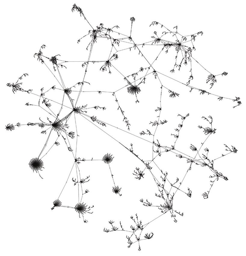
FIGURE 8. Marginal adjacency and Tucker decomposition of reality mining data. Distinct community structure is observed in
the time-marginalized adjacency matrix of the reality mining dataset (a). The three delineated blocks correspond to “General
Graduate,” “MIT Media Lab,” and “Sloan” student clusters respectively. The Tucker decomposition is shown in (b) and (c).
Because of the symmetric property of the adjacency matrix, indices 1 and 2 produce identical projection matrices; therefore,
only one copy is included here for clarity. It is easy to see clear community structures in the social network profiles, most nota-
bly the distinction between Media Lab and Sloan students.
index in the data tensor, this interpretation may be a nating the tensor decomposition. For ease of interpret-
more natural way to interpret a Tucker decomposition as ability, the indices of the input tensor were reordered by
opposed to traditional interpretations of MLSI in which using spectral clustering (as described earlier). To do so,
the list of most active participants from each correlat- the second-largest eigenvector of the normalized graph-
ing pair (or tuple) of indices is returned by the system Laplacian of the time-marginalized social network was
in list form. calculated (Figure 8a). The values in this eigenvector were
To gain insight on the ability of this approach to sum- then sorted, and the resulting reordering of indices was
marize group behavior from dynamic social network data, used to reorder indices in the input tensor.
close-range social interactions were analyzed from the For each dataset, MLSI was performed via a rank-
Reality Mining Project’s corpus. (25, 25, 25) Tucker decomposition of the preprocessed
input tensor, keeping the original time resolution on
Experimental Protocol samples. The size of the decomposition was chosen heu-
For these experiments, the researchers used Bluetooth ristically to represent a reasonable number of profiles
proximity information from periodic scans of nearby users could sort through when interpreting the results.
devices from each of the 94 participants in the reality Both the size of the decomposition and the time reso-
mining study. The proximity information resulted in more lution of the input tensor are open issues when this
dense interaction networks than call data when small approach is used, and a discussion of these issues is
time increments were considered. deferred until the experiment sections. Results were
The number of detections between study partici- generally evaluated qualitatively.
pants per hour was used as the social interaction feature.
Restricting the time range to the academic year (1 Sep- Results
tember 2004 to 15 May 2005) and removing participants The first two of the social profile vectors in Figure 8b
lacking Bluetooth data resulted in a mode-3 data tensor correspond loosely to the two main communities seen
of size 95 × 95 × 6168. That is, for input tensor X, (xi , j, k ) in the Reality Mining Project’s data, namely the Media
corresponds to the number of times participant i was Lab and Sloan participants. Subsequent profile vectors
detected by participant j at hour k. corresponded to the larger, more active Media Lab par-
The values in the input tensor were nominalized by ticipants. In general, researchers observed reasonable
log (1 + xi , j, k )∀xi , j, k to prevent large values from domi- community clustering and co-clustering where it existed.
70 LINCOLN LABORATORY JOURNAL VOLUME 20, NUMBER 1, 2013WILLIAM M. CAMPBELL, CHARLIE K. DAGLI, AND CLIFFORD J. WEINSTEIN
Temporally, the expected gaps in the time pro- SLOAN GRADUATE STUDENTS
files corresponded to the Thanksgiving holiday, 25–29 The most interesting results of the MLSI analysis of the
November [35], and winter break, 18 December–2 Jan- Reality Mining Project’s data were subnetworks (and asso-
uary* [35]. The disbanding of the Sloan School com- ciated time profiles) correlating with the Sloan graduate-
munity as a whole was detected after the fall semester, student community. As can be seen in Figure 9b, both the
and was easily observable in the sharp drop-off of signal Sloan student subnetwork and the corresponding time
energy in time profile 2 as seen in Figure 9b. Additionally, profile were detected cleanly. From the time profile, this
spectral analysis showed that the time profiles exhibited subnetwork appeared strongly only in the fall semester.
behavior corresponding to daily and weekly routines: the Figure 10b lists the most prominent time stamps
two largest spectral components (on average) are 1/24 from each peak cluster (sorted chronologically) from this
hours and 1/163 hours (1/6.8 days). This specific result time profile. Interestingly, the strongest periodic behavior
was also observed by Eagle and Pentland [1]. The time can be observed on Tuesdays and Thursdays at 11:00 a.m.
profiles seen in Figure 8c are more clearly interpreted in from the middle of October to the beginning of Decem-
the context of their correlated subnetworks, which are ber. If one zooms into the time profile, local peaks can be
shown in Figure 9a. observed consistent with this result. Figure 10a shows a
It is instructive to view the results of the MLSI analy- three-week window between 24 October and 22 Novem-
sis with respect to the two main communities represented ber 2004. The red bars on the time axis delineate weekday
among the participants in the study: the Media Lab and from weekend. At this finer time resolution, an additional
Sloan graduate students. weekly subpeak associated with Thursdays at 4:00 p.m.
can be observed. These same spikes on Tuesdays and
MEDIA LAB COMMUNITY Thursdays at 11:00 a.m. and Thursdays at 4:00 p.m.
The first time-profile-specific subnetwork, Figure 9a, appeared locally throughout the profile, not just in weeks
was the most relevant subnetwork for the Media Lab associated with the global peaks.
community, and in general, a compact first-order sum- Because the spikes were clearly periodic, persisted
mary of the data. The time profile exhibited a fairly through the fall semester, and then disappeared in the
uniform structure across all time instances, with gen- spring, the evidence suggested this behavior could be due
eral periodic features consistent with work- and school- to course-attending activity. Of all Sloan course offerings
related activities throughout the academic year. Most in fall 2004 [36], only two courses were consistent with
noticeably, the gap in the time profile corresponded to this behavior. Of these, only the first-year core course,
the break between fall and spring semesters. The subnet- 15.515, Financial Accounting [37], fit all the observed
work showed that the majority of the social interactions evidence. As seen in Figure 10c, 15.515 had three lecture
occurred among the larger Media Lab community (with sessions that met Tuesdays and Thursdays from 10:30
a relatively smaller proportion occurring in the Sloan a.m. to 12:00 p.m., and two recitation sessions that met
community). This information differed from that con- Thursdays at 4:00 p.m. Therefore, one could make the
veyed in the average social network derived from mar- uncertain, yet probable, claim that the behavior observed
ginalizing interactions over time (seen in Figure 8a). in this time profile corresponded to Sloan students
When time information was removed, it appeared the attending 15.515, Financial Accounting.
Sloan community was equally active as the Media Lab This MSLI approach is ideally suited for scenarios in
community during this time period. In reality, as this which actors co-cluster cleanly in space and time. Given
subnetwork and subsequent subnetworks arising from the appropriate context, MSLI analysis allowed research-
tensor analysis showed, this was not the case. ers to establish (with some degree of uncertainty) a causal
link between an observed behavior and a generating event,
a result that was not readily apparent from the input data.
Tensor-based analysis tools such as MLSI are fast,
* Last day before the Independent Activities Period during first-order tools that could allow users to refocus both
the January intersession. their attention and the attention of more resource-inten-
VOLUME 20, NUMBER 1, 2013 LINCOLN LABORATORY JOURNAL 71SOCIAL NETWORK ANALYSIS WITH CONTENT AND GRAPHS
Positively correlated social
interactions for time profile 1 Time profile 1
0.08
10
0.06
20
0.04
30
0.02
40
Strength
Sensor
50
0 (a)
60 –0.02
70 –0.04
80
–0.06
90
–0.08
10 20 30 40 50 60 70 80 90 0 1000 2000 3000 4000 5000 6000 7000
Sensor Time (hr)
Positively correlated social
interactions for time profile 2 Time profile 2
10 0.15
20 0.1
30
0.05
40
Strength
Sensor
50
0 (b)
60 –0.05
70
–0.1
80
–0.15
90
10 20 30 40 50 60 70 80 90 0 1000 2000 3000 4000 5000 6000 7000
Sensor Time (hr)
Positively correlated social
interactions for time profile 3 Time profile 3
0.08
10
0.06
20
0.04
30
0.02
40
Strength
Sensor
50
0 (c)
60 –0.02
70 –0.04
80 –0.06
90 –0.08
10 20 30 40 50 60 70 80 90 0 1000 2000 3000 4000 5000 6000 7000
Sensor Time (hr)
FIGURE 9. Time-profile-specific subnetworks for Reality Mining Project dataset. Subnetworks and
their correlated time profiles are shown in pairs for time profiles 1 (a), 2 (b), and 3 (c) respectively.
Positive and negative values in the time profile indicate positive and negative correlations, respec-
tively, with the associated subnetwork. This representation provides a richer interpretation for com-
munities and their behavior as compared to the results shown in Figure 8.
72 LINCOLN LABORATORY JOURNAL VOLUME 20, NUMBER 1, 2013WILLIAM M. CAMPBELL, CHARLIE K. DAGLI, AND CLIFFORD J. WEINSTEIN
Time profile 2 Thu 11:00:00 07-Oct-2004 15.515 L01 E51-395 TR8.30-10
Thu 16:00:00 14-Oct-2004 15.515 L02 E51-325 TR8.30-10
0.15 Tue 10:00:00 26-Oct-2004 15.515 L04 E51-395 TR10.30-12
Thu 11:00:00 28-Oct-2004
Tue 11:00:00 02-Nov-2004 15.515 L05 E51-325 TR10.30-12
Thu 10:00:00 04-Nov-2004 15.515 L06 E51-315 TR10.30-12
Tue 11:00:00 09-Nov-2004 15.515 R01 E51-151 R3
Tue 11:00:00 16-Nov-2004 15.515 R02 E51-085 R1
Thu 11:00:00 18-Nov-2004 15.515 R03 E51-057 R1
0.1 Tue 11:00:00 23-Nov-2004
Tue 11:00:00 30-Nov-2004 15.515 R04 E51-085 R3
Thu 11:00:00 02-Dec-2004 15.515 R05 E51-085 R4
Strength
Mon 10:00:00 06-Dec-2004 15.515 R06 E51-315 R4
(b) (c)
15.515 Financial Accounting
0.05 Prereq:–
G (Fall)
4-0-5
An intensive introduction to the preparation and interpretation of financial information.
Adopts a decision-maker perspective on accounting by emphasizing the relation between
0 accounting data and the underlying economic events generating them. Class sessions are
a mixture of lecture and case discussion. Assignments include textbook problems,
analysis of financial statements, and cases. Restricted to first-year Sloan Master’s
1300 1400 1500 1600 1700 1800 1900 2000 students.
Time (hr) R. Frankel, G. Plesko
(a) (d)
FIGURE 10. Possible course-attending behavior. The time stamps corresponding to the strongest peaks in time profile 2 (b)
show strong periodic behavior on Tuesdays and Thursdays at 11:00 a.m. Of the two first-year core courses in the fall 2004
course catalog consistent with these times, only 15.515, Financial Accounting (c), looks consistent with the data. Figure 10a
shows local spikes occurring consistently on Tuesdays and Thursdays at 11:00 a.m., as well as minor spikes on Thursdays at
4:00 p.m. (one of two recitation sessions meeting at that time). This behavior persists throughout the fall semester and dis-
appears in the spring. From this analysis, researchers hypothesized the subnetwork corresponding to this time profile could
be those Sloan students attending the first-year core course, 15.515, Financial Accounting (d).
sive analytics, such as relational learning, further down held-out test dataset was used for evaluation, and receiver
the processing chain. operator characteristic (ROC) curves for correct prediction
of leadership were presented. A more complex model was
Relational Learning applied to give improved performance in a more realistic
Prior sections focused on constructing social networks, “data-poor” test condition. Such features can be impor-
finding communities, and analyzing dynamic patterns of tant components of an overall automatic threat detection
activity. This section considers the problem of inference system. In such a system, automatic identification of indi-
on graphs. Given graphs with a rich attribute structure vidual roles and activities from basic features can help infer
and a statistically large sample, it is possible to perform the intent of groups and individuals through higher-level
statistical relational learning on them. These methods pattern recognition and social network analysis.
learn models that relate attributes in a graph neighbor-
hood of a given individual. These Bayesian graphical Graphical Schema
models can be used to impute missing values, perform For the research on predicting leadership roles, Labora-
prediction, and interpret classification results. tory analysts used a subset of the overall ISVG database
Lincoln Laboratory used statistical relational learning schema that contained most of the categorical fields and
algorithms to predict leadership roles of individuals in a continuous variables available in the database. A con-
group on the basis of patterns of activity, communication, tinuous variable may consist of a date, age, number of
and individual attributes [38]. By using labeled training casualties, or other such variables represented by a single
data, analysts applied supervised learning to build a model number. Categorical fields generally represent the type of
that described the structures and patterns of leadership a particular object in the database and may include inci-
roles. The relational model returned a probability that a dent types (e.g., bombing, armed assault, kidnapping)
particular person is in a leadership role, given a graphical or specific information about weapons or bombs used
representation of the individual’s activities and attributes. A in an attack.
VOLUME 20, NUMBER 1, 2013 LINCOLN LABORATORY JOURNAL 73SOCIAL NETWORK ANALYSIS WITH CONTENT AND GRAPHS
Region Operates
within
Region ID
Located Country
Name
within
Country ID
Located State
Name
within
City
State ID Located
Name within City ID
Name
Located
Located
Incident Associate
Located
Incidenttype
Associate Group
Date Involved
Attackpurpose
Located Name
Individual Attacktype
Ideology
Deaths
Region
BirthDate Assaulttarget
Involved
Rank Hostagenationality
Nationality Bombtype
Gender
Education
Member
FIGURE 11. Sample ISVG database schema. Each node in the schema represents an entity type and the available attributes
for that entity. Entities can be linked by relationships of different types. In total, there are 9 node, 90 attribute, and 11 link types.
A sample of the schema is represented graphically in the desired matches and adding annotations to that struc-
Figure 11. Each node represents an object type, and the ture to further refine the query. Matches are returned as
text below the object type represents the available attri- subgraphs, which are small subsections of the overall data
bute fields for each object. For example, individuals have containing only the desired structure.
a “birth date,” “nationality,” “gender,” and other attributes.
Objects are linked via a specific link type indicated by the Methods and Technical Solutions
text on the line. At the center of the schema is the inci- Classification uses statistical methods to predict the status
dent, and groups and individuals connect to particular of an (unknown) characteristic, or feature, of a particu-
incidents via their involvement. The entire dataset con- lar entity given a set of observed characteristics also on
sists of 9 different node types, 90 different attribute types, the entity. Most classification algorithms assume data are
and 11 link types. The actual instantiation of the graphical independent and identically distributed (i.i.d.). However,
database contains more than 180,000 nodes with more because of the connections inherent in social, technologi-
than 2 million attributes spread across the 90 attribute cal, and communication networks, data arising from these
types. Nodes are connected by more than 1 million links. sources do not meet either of these conditions. For exam-
ple, in criminal networks, known associates of convicted
Graphical Query criminals are likely to be criminals as well (noninde-
Once the database was represented as a graph with nodes, pendent), and some criminals have many more associ-
edges, and attributes, QGRAPH software was used to pull ates than others (heterogeneous). Furthermore, network
selected subgraphs from the larger database for analysis. data often exhibit autocorrelation among class labels of
QGRAPH is a graphical query language designed for query- related instances [40]. The concept of autocorrelation,
ing large relational datasets, such as social networks [39]. sometimes called homophily, is best summarized by the
Queries are specified visually by drawing the structure of phrase “birds of a feather flock together,” indicating that
74 LINCOLN LABORATORY JOURNAL VOLUME 20, NUMBER 1, 2013WILLIAM M. CAMPBELL, CHARLIE K. DAGLI, AND CLIFFORD J. WEINSTEIN
individuals with similar characteristics tend to be related. related instances exhibit autocorrelation [44]. Thus, col-
Failure to account for nonindependence and heterogene- lective classification is widely studied within the field of
ity in network data can lead to biases in learned models SRL [45]. Two specific SRL techniques for classification
when traditional approaches are used for classification in relational data are presented here: the relational prob-
[41, 42]. While traditional classification algorithms can ability tree and relational dependency network.
incorporate relational features, an exhaustive aggregation
of relational features becomes less efficient as the dataset RELATIONAL PROBABILITY TREES
becomes large. Even with the incorporation of relational The relational probability tree (RPT) is a probability-esti-
features, the standard classification approach still makes mation tree for classification in relational domains [46]. A
predictions for each instance that are independent, mak- probability-estimation tree is a conditional model similar
ing collective classification more difficult. to a classification tree; however, the leaves contain a prob-
ability distribution rather than a class label assignment
OVERVIEW OF STATISTICAL RELATIONAL LEARNING [47]. To account for nonindependence in network data,
Statistical relational learning (SRL) is a subdiscipline of the RPT is designed to use both intrinsic features on the
the machine learning and data mining communities [43]. target individual and relational features on related indi-
As its name implies, the focus of SRL is extending tradi- viduals. However, because of heterogeneity in the data,
tional machine learning and data mining algorithms for the number of relational features can vary from individ-
use with data stored in multiple relational tables, as typi- ual to individual. To account for possible heterogeneity,
cally occurs in a relational database, such as MySQL or the RPT automatically constructs features by searching
Oracle. This storage model permits analysis of data that over possible aggregations of the training data. The RPT
are nonindependent and heterogeneous, such as social applies standard aggregations—e.g., COUNT, AVERAGE,
network data. The primary focus of this work is classi- MODE—to dynamically flatten the data before selecting
fication in social network data. For example, in criminal features to be included in the model. To find the best
networks, analysts are often interested in predicting a feature, the RPT searches over values and thresholds for
binary variable indicating whether a particular individual each aggregator. For example, to aggregate over criminal
will commit a crime in the near future. The true value of activity of an individual, an appropriate feature might be
this variable is generally unknown at the time of analy- [COUNT(CriminalActivity.type=Larceny) > 1], where the
sis; however, there are a number of observable features type and number are determined by the algorithm. The
that are predictors, such as whether the individual or a RPT has successfully predicted high-risk behavior in the
closely related individual has committed a crime in the securities industry in the United States by using the social
past, has recently filed bankruptcy, or has lost a job. Tools network among individuals in the industry [48, 49].
developed in the SRL community extend the traditional
classification paradigm to include features on both the RELATIONAL DEPENDENCY NETWORKS
individual in question and features on individuals related The relational dependency network (RDN) is a joint rela-
through social or organizational ties. tional model for performing collective classification [50].
In addition to using features on related individuals, An RDN is a pseudolikelihood model consisting of a col-
social network data also provide the opportunity for col- lection of conditional probability distributions (CPD) that
lective classification. Collective classification is possible have been learned independently from data. The CPDs
when many individual class labels (e.g., future crime sta- used in a dependency network are often represented by
tus) are unknown but are connected via social or organi- probability-estimation trees, although any conditional
zational ties. These relations among individuals permit model suffices [51]. Lincoln Laboratory’s work used an
the predictions about one individual to propagate to pre- RDN consisting of a set of individually learned RPTs for
dictions about related individuals. Collective approaches, each attribute that were combined into a single, joint
which infer the value of all unknown labels simultane- model of relational data. Inference (prediction) in the
ously, have been shown to yield higher accuracies than RDN was accomplished by using Gibbs sampling, a tech-
noncollective models, particularly when the labels of nique that relies on repeated sampling from conditional
VOLUME 20, NUMBER 1, 2013 LINCOLN LABORATORY JOURNAL 75SOCIAL NETWORK ANALYSIS WITH CONTENT AND GRAPHS
person incident associate_incident
involved helped
exists exists type = individual
linktype = Involved (incidenttype) [1..]
(rank) [0..]
[1..]
Associate
linktype = Associate [0..]
[1..]
Member_group associate
linktype = Member type =
[1..] individual
[0..]
group associate_group
Member_associate_group
type = type = individual
group linktype = Member
[0..]
[1..]
[0..]
FIGURE 12. Graphical query for leadership. The query looks for all individuals where
the rank is specified (person exists), individuals associated with that person (associate),
incidents and people associated with those incidents (upper box), and groups and groups
associated with those groups (lower box). Nodes indicate entities (people, groups, and
incidents) to look for in the graph. The desired attributes (e.g., “helped”) are specified on
the nodes and edges. Subqueries are indicated using the plate (rectangle). The notation
[n..] indicates that there should be at least n cases of a link or node.
distributions [52]. The RDN can represent autocorrela- learning techniques were applied, highlighting the differ-
tion relationships and was the first joint model that per- ences in data-rich versus data-poor operational conditions.
mitted the learning of autocorrelation relationships from
data. Collective classification was performed via inference LEADERSHIP ROLE PREDICTION
using multiple iterations of Gibbs sampling whenever The ISVG database contains 3854 individuals with labeled
relational features were included in the learned trees. roles. These roles were binned into leadership and non-
leadership categories, and QGRAPH was used to extract
Empirical Evaluation relevant subgraphs for training and testing. There were
Experiments were performed using the ISVG relational 2890 randomly selected subgraphs for training and 964
database. Each of these experiments required a labeled set of for evaluation. The query is shown in Figure 12. The query
subgraphs for training of the relational models and another, looked for persons with a leadership attribute and all of
nonoverlapping set, for evaluation. Using the QGRAPH soft- their associates, including those related through the same
ware, Lincoln Laboratory researchers constructed appropri- group or incident as well as the groups and incidents
ate queries to return these subgraphs and randomly divide themselves. The query in Figure 12 contains two subque-
them into training and test sets using fourfold cross valida- ries (rectangular boxes) that look for zero or more inci-
tion. After the learned model was applied to the evaluation dents and groups, along with individuals involved in the
set on one fold of the randomly selected data, the results incident or members of the group. In this way, the total
were presented in ROC performance curves. number of related individuals was expanded beyond what
The target application was the prediction of leader- the ISVG annotator labeled in the “Associate” link. Addi-
ship attributes of individuals within a group. The ISVG tionally, the incident attributes and group type could indi-
data contains a rich set of individual roles. For the Labo- cate an organizational structure to help predict leadership.
ratory’s research, these roles were binned into categories The first experiment assumed a data-rich condition
pertaining to leadership (e.g., field commander, cell leader, in which full information about neighboring associates is
spiritual leader) and nonleadership (e.g., group member, known (e.g., age, education level, nationality, and so on); see
aide, activist), resulting in a binary classification. Different Figure 13. All of this information was used in the RPT model
76 LINCOLN LABORATORY JOURNAL VOLUME 20, NUMBER 1, 2013You can also read