Projection scrubbing: a more effective, data-driven fMRI denoising method
←
→
Page content transcription
If your browser does not render page correctly, please read the page content below
Projection scrubbing: a more effective, data-driven fMRI
                                                                                          denoising method

                                           Damon Pham1 , Daniel McDonald2 , Lei Ding1 , Mary Beth Nebel3,4 , and Amanda Mejia1
                                                                     1
                                                                         Department of Statistics, Indiana University, Bloomington, IN, USA
                                                          2
                                                              Department of Statistics, University of British Columbia, Vancouver, BC, Canada
                                             3
                                                 Center for Neurodevelopmental and Imaging Research, Kennedy Krieger Institute, Baltimore, MD, USA
arXiv:2108.00319v1 [stat.AP] 31 Jul 2021

                                                                4
                                                                    Department of Neurology, Johns Hopkins University, Baltimore, MD, USA

                                                                                                    Abstract

                                                      Functional MRI (fMRI) data are subject to artifacts arising from a myriad of sources, including
                                                  subject head motion, respiration, heartbeat, scanner drift, and thermal noise. These artifacts cause
                                                  deviations from common distributional assumptions, introduce spatial and temporal outliers, and
                                                  reduce the signal-to-noise ratio of the data—all of which can have negative consequences on the
                                                  accuracy and power of statistical analyses. Scrubbing is a technique for excluding fMRI volumes
                                                  thought to be contaminated by artifacts. Motion scrubbing based on subject head motion derived
                                                  measures, while popular, suffers from a number of drawbacks, among them the need to choose a
                                                  threshold, high rates of scrubbing, consequent exclusion of subjects, and a lack of sensitivity to
                                                  non-motion related artifacts. Data-driven scrubbing methods, which are instead based on observed
                                                  noise in the processed fMRI timeseries, may avoid many of these issues and achieve higher sensitivity
                                                  and specificity to artifacts. Here we present “projection scrubbing”, a new data-driven scrubbing
                                                  method based on a statistical outlier detection framework. Projection scrubbing consists of two
                                                  main steps: projection of the data onto directions likely to represent artifacts, and quantitative
                                                  comparison of each volume’s association with artifactual directions to identify volumes exhibiting
                                                  artifacts. Compared with DVARS, which is also data-driven, a primary advantage of projection
                                                  scrubbing is its use of a common reference to identify abnormal volumes, rather than differences
                                                  between subsequent volumes. We assess the ability of projection scrubbing to improve the reliability
                                                  and predictiveness of functional connectivity (FC) compared with motion scrubbing and DVARS.
                                                  We also compare projection methods, including independent component analysis (ICA), principal
                                                  component analysis (PCA), and a novel fused PCA method. We perform scrubbing in conjunction
                                                  with regression-based denoising through CompCor, which we found to outperform alternative meth-
                                                  ods. Projection scrubbing and DVARS were both substantially more beneficial to FC reliability
                                                  than motion scrubbing, illustrating the advantage of data-driven measures over head motion-based
                                                  measures for identifying contaminated volumes. ICA-based projection scrubbing produced the most

                                                                                                        1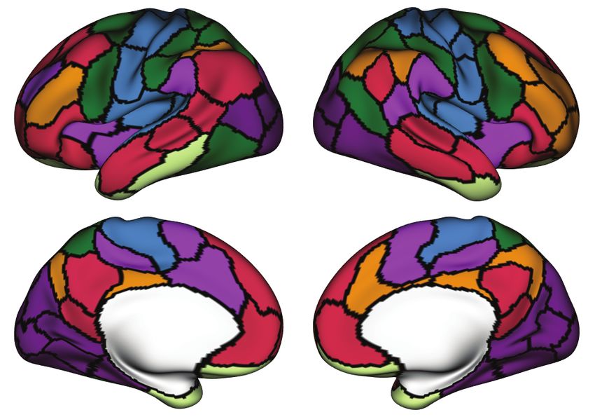
benefit to FC reliability overall. The benefit of scrubbing was strongest for connections between
      subcortical regions and cortical-subcortical connections. Scrubbing with any method did not have a
      noticeable effect on prediction accuracy of sex or total cognition, suggesting that the ultimate effect
      of scrubbing on downstream analysis depends on a number of factors specific to a given analysis.
      To promote the adoption of effective fMRI denoising techniques, all methods are implemented in a
      user-friendly, open-source R package that is compatible with NIFTI- and CIFTI-format data.

1    Introduction

Neuronal activity measured by the blood-oxygen-level dependent (BOLD) signal makes up only a small
component of the total fluctuation in fMRI data (Lindquist, 2008; Bianciardi et al., 2009). A myriad of
artifactual sources of variation cause fMRI data to exhibit low signal-to-noise ratio (SNR) and deviations
from common distributional assumptions—e.g. Gaussianity, stationarity, homoskedasticity—due to ac-
tifacts’ spatiotemporal patterns and variable magnitude. Therefore, it is vital to remove as much noise
from fMRI data as possible prior to statistical analysis. This is a difficult task, because the potential
sources of noise are diverse in their origin and manifestation. For example, artifacts may be introduced
due to subject head motion, physiological processes such as respiration, heartbeat, and blood flow fluc-
tuation, thermal noise, magnetic field non-uniformities, scanner drift, and even prior data pre-processing
steps (Bianciardi et al., 2009; Liu, 2016; Caballero-Gaudes and Reynolds, 2017).

While a single gold standard denoising pipeline for fMRI data has yet to be widely accepted, many meth-
ods for modeling, detecting and removing artifacts have been proposed. These methods can be loosely
grouped into two categories: regression-based methods and “scrubbing” (also known as “censoring” or
“spike regression”). Regression-based methods assume that artifactual fluctuations can be modelled us-
ing external or data-driven sources of information and linearly separated from the data. For example, it
is well-known that head motion induces artifacts (Power et al., 2012; Van Dijk et al., 2012; Satterthwaite
et al., 2012; Yan et al., 2013), so rigid body realignment parameters and their extensions (i.e. higher-order
terms, their derivatives, or the lagged time-courses) are often regressed from the data to minimize noise
coincident with motion (Friston et al., 1996). However, spatially variable spin-history effects introduced
by motion are difficult to model and can persist after the application of such methods (Yancey et al.,
2011). Similarly, BOLD fluctuations caused by respiration and heartbeat can be minimized by measur-
ing the physiological cycles with a pulse oximeter or by estimating them if temporal resolution is high
enough (Le and Hu, 1996; Power et al., 2017; Agrawal et al., 2020) or if phase information is available
(Cheng and Li, 2010). An alternative approach to directly modeling sources of non-neural variability is
to use tissue-based regressors from brain compartments thought to represent noise as a proxy for these
sources, e.g., signals in the cerebrospinal fluid (CSF) and white matter (Behzadi et al., 2007; Muschelli
et al., 2014; Caballero-Gaudes and Reynolds, 2017; Satterthwaite et al., 2019). Removal of the global

                                                        2
signal across the brain parenchyma remains a popular “catch-all” denoising technique due to its ability
to remove noise for which more targeted techniques may lack sensitivity (Power et al., 2014; Ciric et al.,
2017; Parkes et al., 2018b; Satterthwaite et al., 2019) but is controversial due to its potential to worsen
existing artifacts, remove neurologically-relevant variation between subjects and induce anti-correlations
(Liu et al., 2017; Power et al., 2017; Caballero-Gaudes and Reynolds, 2017; Parkes et al., 2018b). Fi-
nally, noise-related signals can be identified via independent component analysis (ICA) using ICA-FIX
(Salimi-Khorshidi et al., 2014) or ICA-AROMA (Pruim et al., 2015) and regressed from the data.
Regression-based methods are effective at mitigating low- and medium-frequency nuisance signals, but
they may be less powerful against “burst noise” caused by sudden head motion, irregular breaths, or
hardware malfunction, which is difficult to model due to its unpredictable incidence and structure (Power
et al., 2012; Yan et al., 2013; Parkes et al., 2018b; Satterthwaite et al., 2019). Therefore, another,
complementary approach is to identify and remove volumes that are highly contaminated, a process
known as scrubbing. The most popular scrubbing techniques are motion scrubbing based on frame-wise
displacement (FD), a summary measure of head movement relative to the the previous volume (Power
et al., 2012, 2014), and DVARS, a measure of the change in image intensity from the previous volume
(Smyser et al., 2010; Power et al., 2012). Both motion scrubbing and DVARS require the choice of a
threshold to identify volumes to remove. Afyouni and Nichols (2018) recently formulated DVARS as
a sum-of-squares decomposition and proposed two DVARS-related measures that can be thresholded
in a principled way. For motion scrubbing, however, there is no principled or universally accepted FD
threshold above which volumes are considered contaminated. While a range of thresholds between 0.2
and 0.5 are commonly used in the literature (Power et al., 2014; Ciric et al., 2017; Afyouni and Nichols,
2018), the rate of scrubbing can vary dramatically across this range, and the downstream effects of
different choices are not well-understood.
While motion scrubbing is arguably the most popular form of scrubbing used in fMRI analyses, it has a
number of disadvantages in addition to the ambiguity of choosing a threshold. First, the percentage of
volumes flagged for removal is often high, particularly for lower (more stringent) FD thresholds, which
can result in unintentional removal of relevant signal. It is also common practice to exclude subjects for
whom too many volumes are scrubbed, so over-aggressive removal of volumes can result in the exclusion
of a substantial number of study participants. Second, recent work has shown that respiratory motion
can artificially inflate head motion estimates and may result in the erroneous removal of volumes not
concurrent with head motion (Fair et al., 2020). These artifacts in head motion estimates may be
present in single-band fMRI data but are exacerbated using multi-band acquisitions (Gratton et al.,
2020). Given the accelerating adoption of multi-band acquisitions and the growing availability of multi-
band fMRI data through the Human Connectome Project (HCP) and other publicly available datasets
adopting HCP-style acquisitions, e.g., the UK Biobank (Miller et al., 2016), the Developing Human
Connectome Project (Hughes et al., 2017), the Adolescent Brain and Cognitive Development (ABCD)
3study (?), and the Baby Connectome Project (Howell et al., 2019), the likelihood of over-aggressive
removal presents a major concern for which there is currently no clear remedy. Furthermore, since
the majority of studies comparing regression-based denoising and scrubbing techniques have focused
on single-band fMRI acquisition (Ciric et al., 2017; Parkes et al., 2018b), the true effects of motion
scrubbing in multi-band fMRI are largely understudied. Third, subject motion may induce artifacts that
persist into subsequent time points. Power et al. (2012) and others have proposed flagging time points
adjacent to high-FD volumes too, but this expansion applies to all high-FD volumes equally and thus
may yield false positives. Finally, FD is computed prior to, and independent of, any denoising strategies,
and therefore may flag volumes that actually exhibit low degrees of noise after regression-based noise
reduction strategies have been applied.
In contrast to FD, data-driven scrubbing metrics can be computed after denoising in order to flag
only those volumes that still exhibit high levels of contamination. Data-driven scrubbing techniques
are also capable of identifying burst noise that is not due to subject head motion. Here we present a
data-driven, statistically principled scrubbing approach known as projection scrubbing. This approach
consists of two main steps. First, the data is projected onto directions likely to represent artifacts
using strategic dimension reduction and selection. Second, each volume’s temporal activity associated
with those directions is formally compared to the distribution across all volumes to identify statistical
abnormalities or spikes representing burst noise (Mejia et al., 2017). By contrast, both FD and DVARS
are based on comparing each volume to only its temporal predecessor. They are therefore also sensitive
to repetition time (TR) (though it is now possible to properly normalize DVARS as proposed by Afyouni
and Nichols (2018)). Projection scrubbing can be combined with robust outlier detection methods at the
second step to enhance sensitivity and specificity in flagging volumes exhibiting statistical abnormalities
(Mejia et al., 2017). We introduce two important improvements to the original projection scrubbing
method proposed by Mejia et al. (2017). First, while the original framework used principal component
analysis (PCA) for the projection step, we consider two alternative techniques that are more effective
at identifying artifactual directions in the data: ICA and a novel technique, FusedPCA. Second, we
propose a kurtosis-based selection method to separate and retain components of artifactual origin from
those more likely to represent neuronal sources.
The goal of this work is two-fold: first, to assess the performance of projection scrubbing compared
with popular scrubbing techniques; and second, to compare its performance using different projections
(PCA, ICA, and FusedPCA) to determine the optimal method. In assessing the performance of each
scrubbing method, it is important to recognize that noise reduction accompanied by drastic loss of
meaningful signal, e.g. due to over-scrubbing, can be detrimental. Indeed, noise reduction strategies
generally must achieve a balance between removal of noise and loss of true signal. We therefore assess
the ability of scrubbing to maximize the presence of the neuronal signal, relative to the noise in the data,
via two indirect measures of SNR in fMRI: the reliability and predictiveness of functional connectivity
4(FC). For reliability, we specifically consider greater reliability to mean a higher proportion of variance
attributable to unique subject-level features, i.e. more individualized FC. We quantify this using the
intra-class correlation coefficient, as in a number of previous studies (e.g., Shehzad et al., 2009; Zuo et al.,
2010; Thomason et al., 2011; Guo et al., 2012; Shirer et al., 2015), and fingerprinting match rate. This
is an important distinction from other reliability metrics such as test-retest mean squared error (MSE)
or correlation, which are effective at assessing noise reduction but do not penalize loss of subject-level
signal. For example, setting FC to a constant value for all subjects would yield an MSE equal to zero, i.e.
perfect reliability. For predictiveness, we consider the ability of FC to predict two measures: biological
sex and total cognitive ability.
The remainder of this paper proceeds as follows. In Section 2, we describe the projection scrubbing
framework, including our FusedPCA dimension reduction technique and novel kurtosis-based approach
for selecting artifactual components. We also describe the reliability and prediction studies performed to
compare projection scrubbing with existing scrubbing techniques. In Section 3, we report the performance
of projection scrubbing, motion scrubbing and DVARS at improving the reliability and predictiveness of
FC. Finally, we conclude with a discussion of our findings, limitations and future directions in Section 4.
2 Methods
2.1 Projection scrubbing
Projection scrubbing is the process of identifying and removing fMRI volumes exhibiting statistically
unusual patterns likely to represent artifacts. The process of projection scrubbing involves projecting
high-dimensional fMRI volumes onto a small number of directions likely to represent artifacts, then
summarizing those directions into a single measure of deviation or outlyingness for each volume that
can be thresholded to identify volumes contaminated with artifacts. This process consists of three steps,
described in turn below: dimension reduction and selection of directions likely to represent artifacts, com-
puting a measure of outlyingness for each volume, and thresholding that measure to identify artifactual
volumes. All steps are implemented in the fMRIscrub R package.
2.1.1 Dimension reduction and selection of artifactual directions
Let T be the duration of the fMRI timeseries, and let V be the number of brain locations included
for analysis. YT ×V is the vectorized fMRI BOLD timeseries, which has undergone basic preprocessing,
typically including rigid body realignment to adjust for participant motion, spatial warping of the data to
a standard space (e.g. distortion correction, co-registration to a high resolution anatomical image), and
optional spatial smoothing. After robustly centering and scaling the timecourse of each brain location
5(which can be voxels in volume space and/or vertices in surface space), we aim to project Y to XT ×Q ,
which represents the timeseries associated with Q latent directions in the data. In Mejia et al. (2017),
PCA was used for this purpose, and the top Q PCs explaining 50% of the data variance were retained.
This choice was based on the observation that a source of severe burst noise (e.g. banding artifacts caused
by head motion) will cause high-variance fluctuations, so its artifact pattern will tend to manifest in a
high-variance PC. Here, we propose several improvements to this original framework to better distinguish
directions representing artifactual variation from those representing neuronal variation: (1) the use of
improved projection methods for better separation of artifactual directions in the data; (2) a principled
method of dimensionality selection; and (3) a novel kurtosis-based method to identify components likely
to represent artifacts. Each of these is described in turn below.
First, we consider two projection techniques to better to identify artifactual directions in the data
compared with the original PCA approach: ICA and FusedPCA. ICA applied to fMRI typically aims
to decompose the data into a set of maximally independent spatial components and a mixing matrix
representing the temporal activity associated with each spatial component. The ability of ICA to separate
fMRI data into spatial sources of neuronal and artifactual origin is well-established (McKeown et al.,
1998). ICA has been used successfully for noise reduction in fMRI, most notably via ICA-FIX (Griffanti
et al., 2014) and ICA-AROMA (Pruim et al., 2015).
FusedPCA is a novel PCA technique that employs a fusion penalty on the principal component time
series. The fusion penalty has two effects: (1) it encourages a small number of larger jumps in the
time series, which may make it easier to detect volumes contaminated with artifacts; and (2) it more
easily finds sequential outliers, a common feature of fMRI artifacts. FusedPCA recognizes that volumes
contaminated by artifacts, as well as those not contaminated by artifacts, tend to occur in sequential
groups. Effectively, the PC scores for volumes in the same category (containing artifacts or free of
artifacts) should be similar but differ dramatically from those in the other category. Thus, FusedPCA
imposes a piecewise-constant constraint on the PC scores such that the scores for the artifactual volumes
are more likely to occur sequentially and are much larger than the PC scores for the non-artifactual
volumes. FusedPCA is a PCA version of constant trend filtering (Tibshirani, 2014; Kim et al., 2009) and
is an instance of the penalized matrix decomposition framework presented in (Witten et al., 2009). The
optimization problem defining FusedPCA and its estimation procedure are described in Appendix A.
Second, for all projection methods, we determine the number of components to estimate automatically
using penalized semi-integrated likelihood (PESEL) (Sobczyk et al., 2017), a Bayesian probabilistic PCA
approach that generalizes and improves upon the popular method of Minka (2000).
Finally, we propose a novel kurtosis-based method for selection of components likely to represent artifacts.
Artifacts caused by burst noise tend to be both severe and transient. Therefore, a component (e.g. IC
or PC) representing an artifactual spatial pattern will have associated timeseries (e.g. IC mixing or PC
6scores) likely containing spikes or outliers at those time points where the artifact exists. The presence of
these outliers alters the distribution of temporal activity associated with that component. In particular,
kurtosis, the standardized fourth moment of a distribution, will be increased by the presence of these
outliers. The kurtosis of a set of values, x = (x1 , . . . , xN ) is computed as
N 4
X xi − x̄
Kurt(x) = − 3,
i=1
s
where x̄ and s are respectively the sample mean and standard deviation of x. The true kurtosis of
Gaussian-distributed data is 0, but sample kurtosis will exhibit sampling variance. Sampling distributions
of kurtosis for Gaussian-distributed data is shown are Appendix Figure B.1. We select those components
whose timeseries have sample kurtosis significantly larger than what would be expected in Gaussian-
distributed data, defined as exceeding the 0.99 quantile of the sampling distribution of kurtosis for a
particular sample size. This corresponds to a probability of 0.01 for a false positive, i.e. falsely selecting
an outlier-free component. As illustrated in Appendix Figure B.1, for time series of long duration
(over T = 1000), it is appropriate to use the theoretical asymptotic sampling distribution of kurtosis to
determine the 0.99 quantile; for shorter time series, we use Monte Carlo simulation.
For kurtosis-based component selection, it is important that the data be detrended prior to projection or
that the component timeseries be directly detrended. Appendix Figure B.2 illustrates the consequences
of failing to detrend properly. Both mean and variance detrending of the component timeseries are
implemented in the fMRIscrub R package. However for the analyses described below, we detrend the
data prior to projection and therefore forego component detrending. Details of our data detrending
procedure are given in Section 2.3.
2.1.2 Quantifying and thresholding outlyingness
Let XT ×Q contain the timeseries associated with the Q high-kurtosis components (PCs or ICs) after
any detrending. Since the selected components are believed to represent artifacts, outliers or spikes in
their associated timeseries can be used to locate the temporal occurrence of artifacts. We compute an
aggregate (multivariate) measure of the temporal outlyingness of each volume, leverage, which can be used
to identify spikes occurring across any of the components or in multiple components. Leverage is defined
as the diagonal entries of the orthogonal projector onto the column space of X, H = X(X> X)−1 X> ,
and is related to Mahalanobis distance. In the linear regression context, H is called the “hat matrix”
and leverage is related to the influence of each observation on the coefficient estimates. In our context,
leverage is an approximation of the influence of each volume on the selected components (Mejia et al.,
2017). Since these components are selected because the are likely to represent artifacts, leverage can be
interpreted as a composite measure of the strength of artifactual signals in each volume.
The final step is to threshold leverage to identify volumes contaminated by artifacts. To determine an
7appropriate threshold, it is important to note that the total leverage over all T volumes is mathematically
fixed at Q. Therefore, the high leverage associated with any outliers will decrease the leverage of all
other volumes. Thus, the mean leverage will always be Q/T , but the leverage of a typical (non-outlying)
volume may be much lower. Therefore, we use the median leverage across all volumes as a reference
value, and consider volumes with leverage greater than a factor of the median to be outliers. Mejia
et al. (2017) considered a range of thresholds between 3 and 8 times the median, and found 4 to be near
optimal. Here, we consider a range of thresholds up to 8 times the median to provide updated evidence
for an appropriate choice of threshold, given the improved methods, different evaluation metrics, and
multi-band data being considered here.
2.2 Alternative scrubbing methods
For comparison, we consider the following alternative scrubbing methods: motion scrubbing using frame-
wise displacement (FD) (Power et al., 2012, 2014) and DVARS (Smyser et al., 2010; Afyouni and Nichols,
2018). While FD is based on head motion and DVARS is based on BOLD signal change, both measure
the change from the previous volume.
Motion Scrubbing. Head motion is estimated by assuming the brain is a rigid body and realigning all
volumes to a chosen reference (e.g., the mean across all volumes). FD is calculated from the rigid body
realignment parameters according to the formula FD(t) = |∆dxt |+|∆dyt |+|∆dzt |+|∆αt |+|∆βt |+|∆γt |,
where ∆qt = qt − qt−1 (Power et al., 2012). At volume t, dxt , dyt and dzt represent the change in the
brain’s estimated position along the x, y and z coordinates, respectively relative to the reference, while
αt , βt and γt represent the estimated rotation of the brain along the surface of a 50-mm-radius sphere
(an approximation of the size of the cerebral cortex) relative to the same reference. Thus, FD(t) is
equal to the sum of absolute changes in the realignment parameters (RPs, also known as the rigid body
coordinates) between volume t and the previous frame. By convention FD(1) = 0. FD thresholds
reported in the literature vary; thus, we consider a range of FD thresholds between 0.2 mm and 1.0 mm.
DVARS Scrubbing. Afyouni and Nichols (2018) propose two variations of DVARS, which can be
thresholded in a principled manner: ZDVARS which measures statistical significance and ∆%DVARS
PV PV
which measures “practical” significance. Define A(t) = V1 v=1 [Yt,v ]2 and D(t) = V1 v=1 [ 12 (Yt,v −
Yt−1,v )]2 . Then the two variations are
D(t) − median(D) D(t) − median(D)
ZDVARS(t) = and ∆%DVARS(t) = × 100%,
shIQR (D) mean(A)
where shIQR estimates standard deviation robustly using the bottom half of the interquartile range (the
first and second quartiles) and a power transformation (d = 3 as selected by Afyouni and Nichols (2018)).
ZDVARS represents a z-score for signal change, whereas ∆%DVARS measures the excess variance in the
8signal change as a percentage of the mean signal change. Following Afyouni and Nichols (2018), we use
an upper-tail 5% Bonferonni FWER significance level as the cutoff for ZDVARS, and 5% as the cutoff
for ∆%DVARS. Only volumes exceeding both cutoffs are flagged by the “dual” DVARS cutoff method.
2.3 Data collection and processing
We analyze resting-state fMRI (rs-fMRI) from the Human Connectome Project (HCP) 1200-subject
release and the HCP Retest Dataset (Van Essen et al., 2013). We use the minimally preprocessed
(MPP) rs-fMRI data (Glasser et al., 2013) for our main analyses, but we include the rs-fMRI data
denoised with ICA-FIX (Griffanti et al., 2014) for comparison. For the reliability study described in
Section 2.4.1 below, we utilize the HCP test-retest data. Forty-five participants were enrolled in both
the main and retest HCP studies, 42 of whom have both MPP and ICA-FIX versions of all rs-fMRI
scans in full duration and are included in the analysis. Each test-retest subject has a total of eight runs
collected across four visits (test session 1, test session 2, retest session 1, and retest session 2), using
two acquisition sequences at each visit (LR and RL phase encoding). For the prediction study described
in Section 2.4.2 below, we use the main HCP dataset, which includes 1,001 subjects with all four runs
collected across two visits using the LR and RL acquisition sequences. Each rs-fMRI run includes 1200
volumes over a duration of approximately 15 minutes (TR = 0.72). The first 15 frames (just over 10
seconds) of each run are removed to account for magnetization stabilization. We analyze the data in
“grayordinates” space resulting from the HCP surface processing pipeline of cortical data combined with
the HCP volume processing pipeline for subcortical and cerebellar structures. This data consists of
91,282 gray matter brain locations across the left and right cortical surfaces, subcortical structures, and
cerebellum.
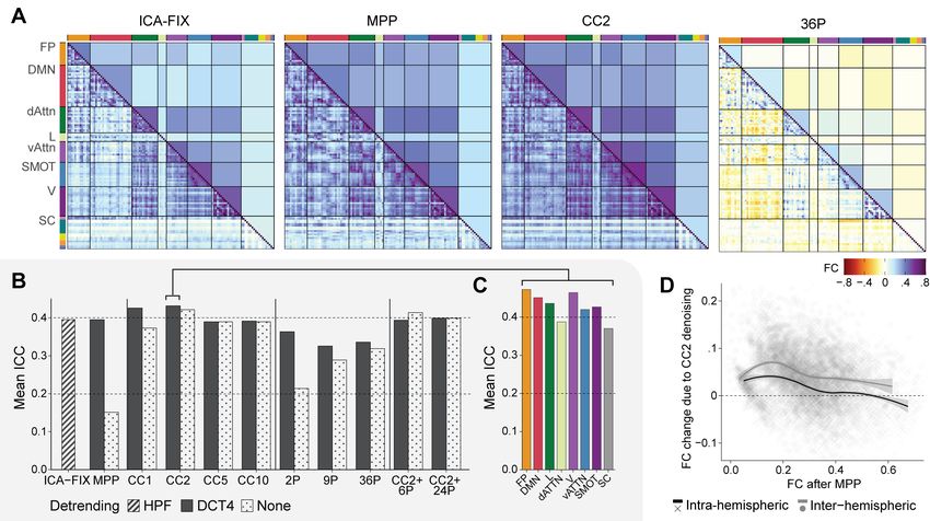
2.3.1 Functional connectivity
In a series of analyses described below, we assess the impact of scrubbing on the reliability and predic-
tiveness of FC. To compute FC, we calculate the average timeseries within each of 100 cortical regions
defined by the Schaefer parcellation and within each of 19 Freesurfer parcels representing subcortical
and cerebellar regions (Figure 1). The 119 × 119 matrix of FC is computed as the Pearson correlation
between each parcel timeseries. Prior to further analyses, a Fisher z-transformation is applied to map
the FC values to the real line. Letting r represent Pearson correlation, the Fisher z-transformation
1
is computed as z = 2 ln {(1 + r)/(1 − r)}. We classify these 119 functional areas into seven cortical
networks based on their overlap with the Yeo et al. (2011) seven-region parcellation and into five sub-
cortical groupings based on location, function, and classical separation between midbrain and hindbrain
structures.
9A B
y = -14 y=3 y = 10
Individual Brainstructures Subcortical Groups
Cerebellum Cerebellum (CBLM)
Accumbens Basal Ganglia (BG)
Caudate Hippocampus−Amygdala (H&A)
Pallidum Brainstem−Diencephalon (B&D)
Putamen Thalamus (TH)
Cortical Networks Amygdala
Frontoparietal Control (FP) Default (DMN) Hippocampus
Dorsal Attention (dATTN) Limbic (L) Brain Stem
Somatomotor (SMOT) Visual (V) Diencephalon
Salience/Ventral Attention (vATTN) Thalamus
Figure 1: Schaefer cortical parcellation and Freesurfer cerebellar and subcortical parcella-
tion. The 100 cortical parcels outlined in black and are grouped based on their overlap with the 7 Yeo
networks (Yeo et al., 2011). Groupings of cerebellar and subcortical structures are indicated using color
gradients. Note that all cerebellar and subcortical regions except the brainstem are separated into left
and right hemisphere in our analysis.
2.3.2 Scrubbing and Denoising
Figure 2 illustrates the data cleaning methods we employ in our comparative analysis of scrubbing
techniques. All cleaning and scrubbing is performed in a simultaneous regression framework to avoid
re-introducing artifacts through sequential processing (Lindquist et al., 2019). First, the original fMRI
data is initially detrended and denoised, as described below. This attenuates trends and certain noise
patterns, providing a lower noise floor and allowing for greater sensitivity of projection scrubbing and
DVARS to burst noise. Second, spike regressors corresponding to volumes to be censored are added to
the matrix of nuisance regressors. The original fMRI data are then simultaneously denoised and scrubbed
using a single regression step.
Data Denoising. Long-lasting noise patterns (e.g. physiological cycles and scanner drift) cannot be
efficiently mitigated by removing individual volumes alone. Regression-based denoising strategies are
therefore complementary to scrubbing, since they remove noise components which last longer than a
few frames. To determine the marginal benefit of scrubbing, we first obtain “baseline” FC estimates
after regression-based denoising alone (indicated in blue in Figure 2). Then we estimate FC again
based on the denoised and scrubbed data (indicated in green in Figure 2). The change in reliability or
predictiveness of the FC estimates compared to the baseline yields the improvement attributable to a
particular scrubbing method.
10FD
Noise
sources
II
Original I Denoised
fMRI data & scrubbed
Nuisance Regression
Leverage
& DVARS
Denoised
Figure 2: Flowchart for fMRI data cleaning. In our processing framework, fMRI data are denoised
in a single simultaneous nuisance regression (blue) which removes shared variance with DCT bases
(yellow) and noise components (orange). For projection scrubbing and DVARS (purple), volumes are
flagged based on the denoised data, and nuisance regression is repeated (green) with a spike regressor
for each flagged volume (purple) added to the design matrix. For motion scrubbing, since FD does not
depend on the fMRI data, the denoised & scrubbed data can be computed directly without a preliminary
nuisance regression.
11Short Description
Name
MPP No additional denoising
CCx Anatomical CompCor based on the top x ∈ {1, . . . , 10} principal components within
masks of cerebral white matter, cerebral spinal fluid (CSF), and cerebellar white
matter in volume space. Two voxel layers are eroded from the white matter ROIs,
and one voxel layer is eroded from the CSF ROI.
2P Mean signals from white matter (cerebral and cerebellar) and CSF. Erosion as in
aCompCor.
9P 2P signals along with the six motion RPs and the global signal. Global signal is
calculated across in-mask voxels in the volumetric MPP data.
36P 9P signals along with their one-back differences, squares, and squared one-back
differences
Table 1: Candidate denoising strategies. All denoising strategies are applied to the minimally
preprocessed (MPP) data via a regression framework using a design matrix including the noise regressors,
an intercept, and (possibly) four DCT bases for detrending and high-pass filtering. The strategy resulting
in the most reliable FC estimates will be adopted as the “baseline” denoising strategy, to be applied
simultaneously with scrubbing.
Since the benefit of scrubbing depends on which denoising strategy is used, we first consider several
options. The strategy yielding the most reliable FC estimates (highest mean ICC, see Section 2.4.1) will
be adopted in subsequent analyses. We consider the following candidate strategies, described in Table
1: no additional denoising (minimal preprocessing, or MPP), anatomical CompCor (CCx), 2 parameter
(P), 9P, and 36P (Behzadi et al., 2007; Satterthwaite et al., 2013a; Muschelli et al., 2014; Satterthwaite
et al., 2019; Parkes et al., 2018b). For each denoising strategy, we also consider including four discrete
cosine transform (DCT) bases for detrending and high-pass filtering. We adopt high-pass rather than
band-pass filtering because removing high-frequency components from rs-fMRI has been shown to worsen
signal-noise separation and reliability of FC estimates (Shirer et al., 2015).
We also include the HCP implementation of ICA-FIX for comparison. The volumetric and surface
BOLD data and 24 motion parameters (6 RPs and their one-back differences, squares, and squared one-
back differences) are all initially detrended with a nonlinear highpass filter. ICA is performed on the
volumetric MPP BOLD data, and noise ICs are identified based on a trained classifier. The noise ICs
are then “softly” regressed from the surface MPP BOLD data, along with 24 RPs, to avoid removing
variance shared with the signal ICs (Griffanti et al., 2014).
Scrubbing. After determining a baseline denoising strategy, we add scrubbing to the regression-based
12data cleaning, as illustrated in Figure 2. The baseline denoised data (blue) is used for computing
DVARS and for identifying outlying volumes using projection scrubbing, i.e., projecting the data onto
artifactual components and computing leverage for each volume. Volumes exceeding a specified threshold
for leverage, DVARS or FD are flagged for removal. We consider a range of thresholds for projection
scrubbing (2 to 8 times the median leverage, in multiples of 1) and FD (0.2 to 1.0 mm, in multiples of
0.1) and choose the one resulting in the most reliable estimates of functional connectivity (highest mean
ICC, see Section 2.4.1).
We perform denoising and scrubbing in a simultaneous regression framework. A second, parallel nuisance
regression on the original MPP data is performed using the same design matrix as in the baseline
denoising, except with a spike regressor column added for each flagged volume (green path in Figure 2).
Finally, flagged volumes are removed from the denoised and scrubbed data. Note that this is equivalent
to censoring the flagged volumes in the MPP data and design matrix prior to the second nuisance
regression.
It is important to note that the final data are obtained through a single simultaneous regression instead
of multiple sequential regressions. This avoids the problem of latter regressors removing orthogonality
between the cleaned data and prior regressors (Lindquist et al., 2019). For example, consider performing
DCT detrending in one regression, followed by another regression with motion realignment parameters
(RPs) estimated from the data prior to DCT detrending. The cleaned data will not necessarily be
orthogonal to the DCT bases after the second regression, meaning that low-frequency trends might have
been re-introduced to the data. Instead, if the DCT bases and RP regressors are combined in a single
design matrix for a simultaneous regression, the cleaned data will be orthogonal to both the DCT bases
and the RP regressors.
2.4 Methods comparison
To compare projection scrubbing with DVARS and motion scrubbing, we assess both the reliability and
predictiveness of FC estimates based on the denoised and scrubbed data. Reliability is assessed using
the intra-class correlation coefficient (ICC) (Shrout and Fleiss, 1979) and fingerprinting match rate.
Predictiveness is based on the accuracy of predicting two demographic/behavioral measures from FC:
biological sex and total cognition. The difference in reliability and predictiveness compared with baseline
denoising yields the marginal improvement attributable to scrubbing.
2.4.1 Reliability study
When large amounts of data are available for individuals (as is the case for each HCP participant included
in our analyses), patterns in FC have been shown to be primarily dominated by organizing principles
13that are common across participants, as well as individual-specific elements of brain networks that are
stable across time (Gratton et al., 2018). Effective noise-reduction strategies will therefore produce FC
estimates that are more stable or reliable across multiple sessions collected from the same subject. Our
metric of reliability, the ICC, can be thought of as a measure of how well an estimate reflects unique
traits in a group of subjects.
To assess the test-retest reliability of FC estimates for each data cleaning strategy, we compute the
ICC(3,1) of the Fisher z-transformed FC values. The ICC(3, 1) is based on the relationship between
mean sum-of-squares between (MSB) and mean sum-of-squares within (MSW). For a given data cleaning
strategy and pair of brain regions, let zij represent the FC estimate for scan j = 1, . . . , J of subject
PJ PJ PN
1
i = 1, . . . , N , let Mi = J1 j=1 zij , and let M̄ = JN j=1 i=1 zij . Then the ICC(3, 1) is given by
MSB − MSW
ICC(3, 1) = ,
MSB + (J − 1)MSW
where
N N J
J X 1 X X
MSB = (Mi − M̄ )2 , and MSW = (zij − Mi )2 .
N −1 i=1
N (J − 1) i=1 j=1
ICC represents a ratio of variances, with ICC = 1 indicating that all of the variance in the estimates
is attributable to between-subject differences, with no variance across repeated measures of the same
individual. At the other extreme, ICC = 0 indicates that all of the variance is attributable to within-
subject variance across repeated measures, with no variance in the underlying measure across subjects.
We adopt ICC(3,1) rather than other ICC measures because it is appropriate for measuring test-retest
reliability when the reliability of a single measurement is of interest (Koo and Li, 2016) and to facilitate
comparison with previous studies of FC reliability (Caceres et al., 2009; Parkes et al., 2018b).
Since previous work has shown FC of individual subjects to be identifiable across multiple sessions (Finn
et al., 2015), we conduct a fingerprinting analysis to assess the extent to which enhanced reliability leads
to enhanced identifiability. That is, does scrubbing improve the fingerprinting match rate? We divide the
eight scans available from each participant into four sets of runs paired by phase encoding acquisition and
visit: the two test LR scans, the two test RL scans, the two retest LR scans, and the two retest RL scans.
For each set of paired runs, fingerprinting is performed using the first scans as the database set and the
second as the target/query set. For each scan in the query set, we calculate Pearson correlations between
its FC and that of each scan in the database set. If the database scan with the highest correlation is from
the same subject, the fingerprint is a match. This procedure is repeated swapping the roles of database
set and query set within each pair to yield eight rounds of matching. The overall match rate is computed
as the rate of successful matches across 8 × 42 total queries. Since previous studies have shown that
using connections only within a certain network can yield more accurate fingerprinting identifications
than using all connections across the brain (Finn et al., 2015), we repeat this procedure using only the
14connections involving each network or the subcortex.
2.4.2 Brain-behavior prediction study
Scientifically useful estimates of FC are those that are not only more reliable, but also more reflective of
demographic and cognitive characteristics of individuals (Finn and Rosenberg, 2021). If subjects’ char-
acteristics can be better predicted using the FC values resulting from a particular data cleaning method,
that method can be thought to better reduce sources of noise, while preserving relevant neuronal signals,
and hence being more predictive of individual characteristics. We predict two demographic variables
available from the HCP: biological sex (“Gender”) and total cognition (“CogTotalComp AgeAdj”). We
chose sex because cognitive function is known to differ between males and females, and there is great
interest in studying the neural basis of these differences (Satterthwaite et al., 2015; Dhamala et al., 2020).
Additionally, many neurobiological disorders impact males and females differently, for instance autism
(Jack et al., 2021; Hernandez et al., 2020), attention deficit hyperactivity disorder (Rosch et al., 2018),
and chronic pain (Fauchon et al., 2021). Thus, reliable methods for investigating sex differences in func-
tional connectivity are needed to delineate the pathophysiology of these conditions. The NIH Cognition
Total Composite Score (referred to as “total cognition” in the HCP behavioral database) (Gershon et al.,
2013; Weintraub et al., 2013) was chosen because data quality has been shown to impact the power of
inter-individual variability in FC to predict inter-individual variability in cognitive performance (Siegel
et al., 2017).
For this analysis, we exclude 18 subjects with fewer than 5 minutes of data remaining after scrubbing
using any method for at least one run, or who had high levels of head motion (FD over 0.3) in at least
half of their volumes across all four runs. We then balance the remaining 983 subjects for sex and motion
within each age group (22 − 25, 26 − 30, 31 − 35 and over 36 years old) by randomly sampling subjects
so that the median FD across males and females is as equal as possible within each age group. The
balanced dataset includes n = 804 (402 female) subjects. For the total cognition prediction model, we
excluded 10 subjects without total cognition scores. Age-adjusted total cognition scores of the remaining
794 subjects range from 88.95 to 153.36, with a mean of 123.36 and a median of 121.58.
For both sex and total cognition, we use a regression framework with a variable selection penalty. For
sex prediction, we use an elastic net penalty that encourages coefficient shrinkage as well as variable
selection (Zou and Hastie, 2005; Friedman et al., 2010). The elastic net is a convex combination of
LASSO (Tibshirani, 1996) and ridge penalties (Hoerl and Kennard, 1970) and usually combines strength
from both for superior predictive accuracy. For total cognition prediction, we use ridge regression,
since empirically we observe virtually no sparsity in the coefficients. For prediction of sex we use a
logistic regression model; for prediction of total cognition we use a linear regression model with Gaussian
errors. We predict total cognition separately for males and females, since the neurobiological correlates of
15intelligence have been shown to vary in both pattern and strength by sex (Jiang et al., 2020a,b; Dhamala
et al., 2021). We employ a nested cross-validation (CV) procedure to obtain out-of-sample predictions
for each subject and session. The predictions are compared to the true values using standard measures of
error: deviance (or log-loss) for sex and MSE for total cognition. Details of the cross-validation procedure
are given in Appendix C. For obtain a set of coefficient values for each method, we re-estimate the model
using all subjects and sessions.
3 Results
3.1 Selection of baseline denoising strategy and scrubbing thresholds
Figure 3 displays the effect of different baseline denoising strategies on the strength and reliability of
FC. Figure 3A displays average FC estimates across all subjects and sessions. Here we display just
four of the denoising strategies for the sake of space: ICA-FIX, as it is provided by the HCP and is a
popular ICA-based denoising method; minimal preprocessing (MPP), since all regression-based denoising
is applied on top of the MPP data; CompCor2 (CC2) since it exhibited the best performance overall,
as described below; and 36P since it illustrates the effect of including global signal regression. Both
CC2 and 36P include detrending with 4 DCT bases. We observe two primary trends: first, we see
clear differences in FC strength across methods, with CC2 having stronger connections than MPP or
ICA-FIX, and 36P inducing off-diagonal negative FC values (e.g., between regions belonging to different
functional networks) due to the inclusion of the global signal (Murphy et al., 2009). The strengthening
of FC with CC2 relative to MPP is likely due to an improvement in signal-to-noise. The effect can be
seen across the entire matrix of FC but is particularly noticeable for connections involving subcortical
regions. Second, a checkerboard pattern of FC can be seen within network pairs (within the diagonal
and off-diagonal blocks), particularly for the MPP data, suggesting differences in FC strength for intra-
and inter-hemispheric connections. This pattern is attenuated or removed by CC2, explored further in
panel (D).
Figure 3B examines the effect of different denoising strategies on the reliability of FC, in terms of the
mean ICC across all connections. First, we observe that DCT4 detrending is nearly uniformly beneficial
for reliability. It tends to yield greater improvement when combined with less effective denoising strate-
gies. This may reflect differences across strategies in the level of implicit detrending they perform. For
example, the MPP and 2P denoising show dramatic improvements to reliability with DCT4, suggesting
that these methods may not achieve effective detrending on their own. From this point forward, DCT4
is assumed to be included in the data cleaning framework unless stated otherwise. The most reliable FC
estimates are produced with low-order aCompCor denoising, with CC2 having the highest mean ICC.
We also consider two extensions of CC2 to assess whether including motion parameters in addition to
16Figure 3: Effects of different denoising methods on the strength and reliability of functional
connectivity. (A) Average FC estimates across subjects and sessions for different denoising strategies,
from left to right: ICA-FIX, minimally preprocessed (MPP), CompCor with two components (CC2), and
the 36 parameter model (36P). CC2 and 36P include detrending with four discrete cosine transform bases
(DCT4). The rows and columns of each matrix represent the 119 regions, which are grouped primarily
by network with subcortical regions last, and secondarily by hemisphere (left then right) (see Figure 1 for
the subcortical legend). The upper triangle of each matrix displays average FC values for each network
pair. (B) Effect of denoising on reliability of FC, in terms of the mean ICC across all connections. Based
on these results, CC2 + DCT4 is adopted as the baseline denoising strategy in subsequent analyses. (C)
Average reliability of connections involving each network after baseline denoising (CC2 + DCT4). (D)
Effect of baseline denoising (CC2 + DCT4) on FC strength for inter- and intra-hemispheric cortical and
subcortical connections. Each point represents a pair of parcels, and lines represent lowess smoothers
with standard errors. Weaker connections and inter-hemispheric connections tend to be strengthened
more by denoising.
17white matter and CSF-derived signals results in more reliable FC. Specifically, we consider the inclusion
of 6 RPs (CC2+6P) or those parameters along with their one-back differences, squares, and squared
one-back differences (CC2+24P). In both cases, we observe worsened reliability compared with CC2
without motion parameters. Thus, we adopt CC2 as the baseline denoising strategy for all subsequent
analyses.
Figure 3C displays the average reliability of connections involving each network after denoising with
CC2. This shows that there are baseline differences in reliability prior to scrubbing, with the most
reliable connections being those involving the fronto-parietal, attention and default mode networks, and
the least reliable connections involving the limbic network and subcortical/cerebellar regions. Figure
3D explores the effect of denoising with CC2 on FC strength for intra- and inter-hemispheric cortical and
subcortical connections. Two effects are clearly apparent. First, weak connections (below 0.3) tend to be
strengthened the most by denoising. Second, inter-hemispheric connections are strengthened more than
intra-hemispheric connections. This explains the near-elimination of the checkerboard pattern observed
in the MPP matrix in Figure 3A. Thus, denoising may help to alleviate noise-related attenuation of
long-range connections.
Figure 4 examines the effect of different thresholds for FD and leverage on both the reliability of FC and
on the proportion of volumes removed. For DVARS, we adopt the dual cutoff as described in (Afyouni
and Nichols, 2018), which results in mean ICC improvement of 0.0057 and removal of 2.5% of frames
on average. For FD, the most reliable FC estimates are produced using a threshold of 0.3 mm, which
results in removal of approximately 10% volumes on average. We therefore adopt this value, which is
between the “lenient” (0.5 mm) “stringent” (0.2 mm) cutoffs characterized by (Power et al., 2014) and
is in the neighborhood of values often adopted in the literature.
For projection scrubbing, we consider all three projection methods (ICA, PCA and FusedPCA) described
above. While they exhibit similar reliability and removal rates, the highest overall reliability is achieved
with ICA and FusedPCA at a threshold of 3 times the median. Note that similar reliability is achieved
with a threshold of 4 times the median, which was recommended by Mejia et al. (2017). We therefore
adopt a cutoff of 3, which results in approximately 3−4% of volumes being removed on average, depending
on the projection. Notably, projection scrubbing removes fewer than half the number of volumes than
motion scrubbing, yet achieves more than double the improvement to reliability. Compared with DVARS,
projection scrubbing removes slightly more volumes but results in more overall improvement to reliability.
Projection scrubbing will be compared in more detail with DVARS and motion scrubbing in subsequent
analysis, but these high-level findings suggest that it tends to produce the most reliable FC estimates
overall. From this point forward, we consider only the ICA and FusedPCA projection methods, since
they tend to outperform the original PCA-based approach.
It is important to ensure that sufficient data remains for each scan (Ciric et al., 2017; Parkes et al.,
18A Motion Scrubbing B Projection scrubbing
.010 .010
ICC improvement
.000 .000
−.005 −.005
0.2 0.4 0.6 0.8 1.0 2 4 6 8
50% 50%
% frames removed
10% 10%
5% 5%
1% 1%
0% 0%
0.2 0.4 0.6 0.8 1.0 2 4 6 8
FD cutoff Leverage cutoff
ICA PCA Fused PCA
Figure 4: Selection of scrubbing thresholds. (A) We consider FD cutoffs between 0.2 and 1.0
mm in multiples of 0.1 mm. A threshold of 0.3 mm (indicated by the vertical gray line) results in the
greatest improvement to FC reliability. At this threshold, approximately 10% of volumes are scrubbed on
average. (B) For projection scrubbing, we consider leverage cutoffs between 2 and 8 times the median,
in multiples of 1. A threshold of 3-times the median (indicated by the vertical gray line) results in the
greatest improvement to FC reliability for all three projection methods (ICA, FusedPCA and PCA).
At this threshold, 3 − 4% of volumes are scrubbed on average, depending on the projection. Notably,
leverage scrubbing censors fewer than half the number of volumes as motion scrubbing, while producing
more than double the improvement to overall reliability.
19A B
5000
Total Volumes Censored
(out of 9600)
4000 900
3000
600
2000
300
1000
0 0
Subjects Subjects
Scrubbing Method Projection (ICA) (both) Motion Scrubbing Method Projection (ICA) (both) DVARS
Figure 5: Overlap between ICA projection scrubbing and other scrubbing methods. (A)
The number of volumes flagged per subject by motion scrubbing, projection scrubbing, or both. Motion
scrubbing tends to flag a much larger number of volumes compared with projection scrubbing. The over-
lap between volumes flagged with projection scrubbing versus motion scrubbing is fairly small. Similar
patterns of overlap with motion scrubbing are seen for DVARS and FusedPCA projection scrubbing (re-
sults not shown). (B) The number of volumes flagged per subject by DVARS, projection scrubbing, or
both. The overlap between DVARS and projection scrubbing is moderate, though a substantial number
of volumes are flagged by only one but not both methods.
2018a). For projection scrubbing and DVARS, all scans had at least 900 volumes (75%, or 10 minutes)
remaining after scrubbing. For FD, only three of 336 total scans had fewer than 5 minutes remaining
after scrubbing, and all scans retained at least 350 volumes (30%, or 4.2 minutes). Thus, we did not
omit any scans from our study on the basis of excessive scrubbing.
Figure 5 examines the overlap between volumes flagged with projection scrubbing and those flagged
with motion scrubbing and DVARS. We only consider ICA projection scrubbing here for brevity, but
FusedPCA projection scrubbing shows similar patterns of overlap. There is strikingly little overlap
between projection scrubbing and motion scrubbing, shown in Figure 5A. Motion scrubbing typically
flags a much higher number of volumes. Using projection scrubbing, only a small portion of high-FD
volumes are typically flagged, and a majority of the volumes flagged are not associated with high levels
of head motion. Patterns of overlap with motion scrubbing are similar for DVARS (results not shown).
This suggests two fundamental differences between motion scrubbing and data-driven scrubbing such as
DVARS and projection scrubbing: first, many volumes with high FD do not exhibit abnormal patterns
of intensity after denoising; second, many volumes without high FD exhibit abnormalities, likely due to
other sources of artifacts.
Considering the overlap between projection scrubbing and DVARS shown in Figure 5B, the two methods
often flag a large number of common volumes. However, for most subjects there is a substantial portion
of volumes identified by only one technique, showing that the two methods work in different ways and
20Figure 6: Effect of scrubbing on FC reliability and strength. (A) The average change in ICC
(over baseline CC2 denoising) across all connections involving a given network or subcortical group.
Projection scrubbing produces greater improvement to FC reliability than DVARS or motion scrubbing
across nearly all networks and subcortical groups. (B) Effect of scrubbing on reliability of FC for
cortical-cortical (C-C) connections, cortical-subcortical (C-SC) connections, and subcortical-subcortical
(SC-SC) connections. Connections involving subcortical regions (SC-SC and C-SC) tend to enjoy the
greatest improvement in reliability due to scrubbing. (C) Effect of ICA-based projection scrubbing
on FC strength. Split violin plots display the distribution of change in FC strength due to scrubbing
for all within-network intra- and inter-hemispheric connections. Vertical bars within each violin half
indicate the mean value. On average, scrubbing increases the strength of inter-hemispheric FC relative
to intra-hemispheric FC.
produce different results, even though they have fairly similar rates of scrubbing, and similar effects on
overall reliability of FC as described below.
3.2 Reliability study results
Figure 6 displays the effects of different scrubbing methods on the reliability of FC, relative to baseline
denoising with CC2. Figure 6A shows the average change in ICC across all connections involving
a particular network. Generally, scrubbing tends to improve reliability of FC for nearly all networks.
Second, projection scrubbing with ICA or FusedPCA tends to improve reliability of FC the most, followed
by DVARS, with motion scrubbing showing the worst performance across all networks with the exception
of the visual network, which is affected negligibly by scrubbing in general. Third, scrubbing results in the
most dramatic improvements in FC reliability for connections involving cerebellar and subcortical areas.
Strong improvements are also observed for connections involving the limbic, ventral attention, and fronto-
21You can also read