Proxy surrogate reconstructions for Europe and the estimation of their uncertainties - Recent
←
→
Page content transcription
If your browser does not render page correctly, please read the page content below
Clim. Past, 16, 341–369, 2020
https://doi.org/10.5194/cp-16-341-2020
© Author(s) 2020. This work is distributed under
the Creative Commons Attribution 4.0 License.

Proxy surrogate reconstructions for Europe and the
estimation of their uncertainties
Oliver Bothe and Eduardo Zorita
Helmholtz Zentrum Geesthacht, Institute of Coastal Research, 21502 Geesthacht, Germany

Correspondence: Oliver Bothe (ol.bothe@gmail.com)

Received: 3 July 2019 – Discussion started: 5 July 2019
Revised: 10 January 2020 – Accepted: 21 January 2020 – Published: 18 February 2020

Abstract. Combining proxy information and climate model          1   Introduction
simulations reconciles these sources of information about
past climates. This, in turn, strengthens our understanding      There have been numerous efforts to reconstruct regional to
of past climatic changes. The analogue or proxy surrogate        global surface temperature for the last 500 to 2000 years.
reconstruction method is a computationally cheap data as-        Many of the statistical reconstruction methods essentially as-
similation approach, which searches in a pool of simulated       sume a linear relationship between proxy information and
climate states the best fit to proxy data. We use the ap-        temperature data. Here, we apply a non-linear method, the
proach to reconstruct European summer mean temperature           analogue method, to reconstruct the mean European summer
from the 13th century until present using the Euro 2k set of     temperature over the past 750 years in annual resolution. Our
proxy records and a pool of global climate simulation output     main goal is to provide a perspective on estimating uncertain-
fields. Our focus is on quantifying the uncertainty of the re-   ties for reconstructions by analogue, which only few previ-
construction, because previous applications of the analogue      ous applications quantified. Our approach relies on a collec-
method rarely provided uncertainty ranges. We show several       tion of dendroclimatological proxy records and the output of
ways of estimating reconstruction uncertainty for the ana-       paleoclimate simulations.
logue method, which take into account the non-climate part          The core of the analogue method is the search for simi-
of the variability in each proxy record.                         lar spatial patterns in simulated temperature data compared
   In general, our reconstruction agrees well at multi-decadal   to the proxy records. That is, we search for simulated ana-
timescales with the Euro 2k reconstruction, which was con-       logues of the climate anomalies indicated by the set of prox-
ducted with two different statistical methods and no infor-      ies at each available date. The method originated during
mation from model simulations. In both methodological ap-        the Second World War when the US Air Force catalogued
proaches, the decades around the year 1600 CE were the           weather situations of previous decades as a means of long-
coldest. However, the approaches disagree on the warmest         range weather forecasting. In this approach, forecasters ob-
pre-industrial periods. The reconstructions from the analogue    tain forecasts by analogy between current observations and a
method also represent the local variations of the observed       past set of weather patterns (Namias, 1948). Lorenz (1969)
proxies. The diverse uncertainty estimates obtained from our     was the first to mention the method in the wider academic
analogue approaches can be locally larger or smaller than the    literature. The analogue method found subsequent applica-
estimates from the Euro 2k effort. Local uncertainties of the    tions in downscaling and upscaling of climate information
temperature reconstructions tend to be large in areas that are   (e.g., Zorita and von Storch, 1999; Schenk and Zorita, 2012).
poorly covered by the proxy records. Uncertainties highlight     Modern analogue techniques of paleoecology follow a simi-
the ambiguity of field-based reconstructions constrained by      lar idea (e.g., Graumlich, 1993; Jackson and Williams, 2004).
a limited set of proxies.                                           The approach allows to reconcile the spatially sparse in-
                                                                 formation from environmental and documentary proxy data
                                                                 with spatially complete and dynamically consistent infor-
                                                                 mation from observational data or long climate simulations

Published by Copernicus Publications on behalf of the European Geosciences Union.
342                                                     O. Bothe and E. Zorita: Uncertainty of proxy surrogate reconstructions

in the sense of data assimilation (Graham et al., 2007;             of reconstructed climate. On the other hand, it allows to pro-
Trouet et al., 2009; Guiot et al., 2010; Franke et al., 2010;       vide alternative reconstructions that are compatible with the
Luterbacher et al., 2010; Schenk and Zorita, 2012; Gómez-           sparse information from the proxy records. The procedure
Navarro et al., 2015b, 2017; Diaz et al., 2016; Jensen et al.,      further acknowledges the possibility that the analogue pool
2018; Talento et al., 2019; Neukom et al., 2019; Wahl et al.,       does not cover certain points in the predictor space. Our pro-
2019). It can provide an initial dynamic understanding of           posed uncertainty estimates originate in the uncertainty of
past climate variability. However, it is less sophisticated than    the individual proxies, whereas Neukom et al. (2019) quan-
full data assimilation procedures (compare, e.g., Tardif et al.,    tify the variations in reconstruction results by using less in-
2019, and discussions in Gómez-Navarro et al., 2017). Gra-          formation than available.
ham et al. (2007) call reconstructions by analogue “proxy              Recent continental proxy-based reconstructions (PAGES
surrogate reconstructions” in an early paleoclimatological          2k Consortium, 2013a) and the underlying proxy predic-
application. Later studies use the approach for climate index       tors are potential test cases and allow to assess the ana-
and climate field reconstructions (e.g., Franke et al., 2010;       logue method against more common reconstruction proce-
Trouet et al., 2009; Gómez-Navarro et al., 2015b, 2017;             dures. (Dis)agreement between the analogue reconstructions
Jensen et al., 2018; Talento et al., 2019; Neukom et al., 2019).    and previously published estimates helps to reevaluate our
   The analogue method is generally found to perform well,          confidence in our understanding of past climate changes. For
e.g., for area-averaged indices and also at the locations of the    the present purpose, we choose the European reconstruction
used predictors (compare, e.g., Franke et al., 2010). However,      from PAGES 2k Consortium (2013a) as a single test case.
reducing the number of predictors prominently worsens the           See also the work by Luterbacher et al. (2016), who discuss
skill at remote locations, and reconstruction skill accumu-         the methods and the proxy selection in more detail. Luter-
lates at the predictor locations (Franke et al., 2010; Gómez-       bacher et al. (2016) rigorously select proxy records of high
Navarro et al., 2015b). Annan and Hargreaves (2012) found a         quality for their reconstruction.
trade-off between accuracy and reliability of reconstructions          In the following, first, we introduce our approach to the
dependent on quality and quantity of the available proxy            analogue search uncertainty as well as the used proxy and
records. They tested a particle filter method. As simple ana-       model data. Then, we discuss the results for three different
logue searches and particle filter methods share common as-         approaches to an analogue reconstruction. These are (i) using
sumptions, this also applies for analogue search reconstruc-        a single best analogue, (ii) using a fixed number of good ana-
tions. Similarly, it is well established that applications of the   logues, and (iii) considering all analogues complying with
analogue method have to deal with a trade-off between ac-           the proxies within a fixed level of uncertainty. We also con-
curacy and variability (Gómez-Navarro et al., 2015b, 2017).         sider estimates from an ensemble following the subsampling
Franke et al. (2010), Gómez-Navarro et al. (2015b), and Tal-        approach of Neukom et al. (2019). We compare the resulting
ento et al. (2019) discuss the influence of considering more        uncertainties among each other, consider general character-
than one analogue to produce a composite reconstruction,            istics of the different reconstructions, and shortly compare
while Graham et al. (2007) and Trouet et al. (2009) consider        reconstructions to records based on station data.
only the single best analogue based on specific criteria. In
any application, one has to consider the potential biases in
the simulation data.                                                2     Methods and data
   Previous analogue search reconstructions do not usually
consider the uncertainty in the predictor data, and studies         2.1     Methods
rarely provide an uncertainty estimate for the final recon-         2.1.1    Analogue search reconstructions
struction. This precludes to some extent a realistic evalua-
tion of predictors or reconstructions. Exceptions are the stud-     The paradigm that past analogues may provide information
ies by Jensen et al. (2018) and Neukom et al. (2019). The           for anthropogenic climate changes is pervasive in climate sci-
former use age-uncertain proxies and obtain an uncertainty          ence (Dahl-Jensen et al., 2015; Schmidt, 2010; Schmidt et al.,
estimate of their reconstruction for Marine Isotope Stage 3         2014) but the origin of the analogue method lies in weather
through shifting the dates of individual proxies (Jensen et al.,    forecasting (see, e.g., Lorenz, 1969). Zorita and von Storch
2018). The latter use a subsampling approach to provide an          (1999) show the method’s value for downscaling, while oth-
ensemble of reconstructions for the Common Era of the last          ers provide evidence for its ability to upscale local informa-
2000 years (Neukom et al., 2019). Their study interprets the        tion (e.g., Schenk and Zorita, 2012; Luterbacher et al., 2010;
spread as uncertainty of the final reconstruction.                  Franke et al., 2010).
   Here, we propose alternative means to estimate the uncer-           Here, we obtain annually resolved large-scale fields of sea-
tainty of analogue search reconstructions based on the cali-        sonal mean summer (June, July, and August; JJA) tempera-
bration correlation of the proxy predictors with an appropri-       ture based on a pool of relevant candidate fields and a set
ate observational dataset. Our approach to estimating uncer-        of local data indices as predictors for the period of 1260 to
tainty ranges reduces the possibility of producing time series      2003 of the Common Era (CE). The reconstruction domain

Clim. Past, 16, 341–369, 2020                                                                  www.clim-past.net/16/341/2020/

O. Bothe and E. Zorita: Uncertainty of proxy surrogate reconstructions                                                         343

                                                                     est and then provide a reconstruction for each date using this
                                                                     minimum number of analogues. Finally, we fix the value of
                                                                     the uncertainty level around the predictors and consider all
                                                                     valid analogues within this uncertainty level.
                                                                        We consider predictors and analogues normalized by their
                                                                     local standard deviation to conserve the interfield relations.
                                                                     The final reconstructions are rescaled by a chosen standard
                                                                     deviation, which is, here, usually the local full-period stan-
                                                                     dard deviation of one of the simulations.

                                                                     2.1.2   Assumptions on uncertainty
                                                                     Empirical reconstructions of past environmental conditions
                                                                     rely on proxy data, which may be documentary notations but
                                                                     more often are measurements of biological, geological, or
                                                                     chemical properties of the environment. Such proxy repre-
                                                                     sentations of the past conditions are naturally uncertain. A
Figure 1. Reconstruction domain and locations of the included        prominent source of uncertainty is that the archives recorded
proxies. Red squares show the proxies included in our search, grey   signals from more than one climate or environmental variable
squares show the locations from the original Euro 2k setup which     (e.g., temperature and precipitation; compare Evans et al.,
we exclude. The grey shaded box shows the original domain of Do-     2013; Evans et al., 2014; Tolwinski-Ward et al., 2013, 2015).
brovolný et al. (2010).                                                 In the following, we describe our thinking on the uncer-
                                                                     tainty of an analogue reconstruction. We first provide gen-
                                                                     eral derivations before describing the three reconstruction ap-
is Europe from − 10 to 40◦ E and from 35 to 70◦ N (Fig. 1).          proaches of (i) best analogue, (ii) fixed number of analogues,
The predictors are proxy reconstructions in temperature units        and (iii) fixed uncertainty level. Our derivation of the uncer-
from the PAGES 2k Consortium (2013a), and the pool of can-           tainty estimates relies on a number of assumptions, which we
didate fields consists of more than 9000 summer temperature          detail in the next paragraphs. Table 1 lists all mathematical
fields from simulations with an Earth system model (Jung-            expressions used in the following.
claus et al., 2010).
   The approach of an analogue search is usually that, for           Derivation of the uncertainty estimates
each set of predictors, i.e., each point in time, one ranks all
                                                                     Correlations provide a simple measure of the relation be-
potential analogues according to a criterion of similarity to
                                                                     tween proxy observations and the climatic environment over
the target proxy pattern. The criterion is traditionally the Eu-
                                                                     a period when reliable (instrumental) observations of the cli-
clidean distance and only the single pool member with the
                                                                     matic variability exist. We assume we can derive the uncer-
smallest Euclidean (e.g., Franke et al., 2010) or a low num-
                                                                     tainty of how well a local proxy record represents the local
ber of so-defined best analogues is considered. It is possible
                                                                     climate from the correlation coefficients. We denote this un-
to weight the found analogues, e.g., according to their dis-
                                                                     certainty hereafter as proxy uncertainty. We use correlations
tance. This can provide more reliable posterior distributions
                                                                     between the proxy records and the observational gridded Cli-
about the climate state.
                                                                     mate Research Unit (CRU) data (Harris et al., 2014, CRU TS
   The approach presented here differs from previous appli-
                                                                     version 3.10). Table 2 in Sect. 2.2 lists the used proxies and
cations in some important aspects. While we also show a sin-
                                                                     their correlations to the observational data. These listed cor-
gle best-analogue reconstruction and a reconstruction based
                                                                     relations enter our considerations on uncertainty.
on a fixed number of analogues, we add a reconstruction that
                                                                        In our present approach, we consider normalized proxy
explicitly considers the uncertainty of the proxy records in
                                                                     data. That is, the variance of an individual proxy i is Vari =
the selection of the analogue fields.
                                                                     1. We also consider normalized simulated records, and their
   The next subsection provides details on our three different
                                                                     local variance then also is Varsim = 1. Our goal is to derive
approaches. In short, first, the single best reconstruction is the
                                                                     a simple criterion for the similarity between proxy patterns
common application, and our uncertainty estimates are de-
                                                                     and simulated (analogue) patterns that takes into account the
rived from the local correlation between gridded observation
                                                                     inherent uncertainty in the proxy records.
data and the local proxy series. Second, a further common
                                                                        Assuming one can interpret the squared correlation coef-
approach is to use a fixed number of analogues. As we want
                                                                     ficient (R 2 ) as explained variance, one can profit from the
to consider the uncertainty of the local predictors, we iden-
                                                                     equivalence:
tify for a given uncertainty level of the proxies the smallest
number of valid analogues for any date in our period of inter-       R 2 = 1 − Varres /Vartot ,                                 (1)

www.clim-past.net/16/341/2020/                                                                    Clim. Past, 16, 341–369, 2020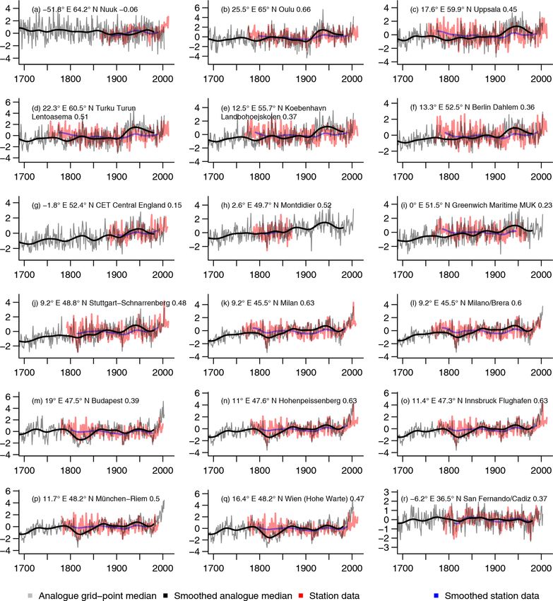
344                                                       O. Bothe and E. Zorita: Uncertainty of proxy surrogate reconstructions

Table 1. List of mathematical expressions.                              We assume these represent 1 standard deviation uncertain-
                                                                        ties. However, they are only an approximation of the uncer-
    Expression    Description                                           tainty. From these, we calculate the assumed standard de-
    r             Correlation coefficient
                                                                        viation intervals, e.g., 2 standard deviations. These are con-
    R2            Squared correlation coefficient                       stant estimates over the full period. If we want to plot the
    Varres        Residual variance                                     time series in temperature units, we have to rescale these es-
    Vartot        Total variance                                        timates. We do this simply by multiplying the noise variances
    Varsig        Variance of the signal                                in the square root by the grid-point variance from a selected
    Varnoi        Variance of the noise                                 simulation. Secondly, our visualizations for the single best-
    Varnoii       Variance of the noise of an individual record         analogue reconstruction add an alternative uncertainty enve-
    Varsim        Variance of a simulation record                       lope. This is given by the mean squared error between the
    Vari          Variance of an individual time series                 proxy values and the best-analogue values at the closest grid
    SD            Standard deviation                                    point. This uncertainty envelope varies over time.
    SDnoi         Standard deviation of the noise                          From our point of view, the real benefit of our derivation
                                                                        of uncertainty is to use only analogues which comply with
                                                                        a certain tolerance criterion. That is, a second way towards
The subscripts are res for residual and tot for total.                  an uncertainty estimate assumes that we can obtain a similar-
  We can take the total variance Vartot to be equal to the              ity criterion between proxy data and simulation pool by con-
variance of the sum of a signal (subscript sig) and the residual        sidering the noise standard deviation for an individual proxy
noise. If we assume these are uncorrelated, we obtain                   as a local noise tolerance threshold. A candidate field has to
                                                                        comply with all local thresholds to be considered a valid ana-
1 − R 2 = Varnoi /(Varsig + Varnoi ).                             (2)   logue. We then can limit our analogue search to only those
                                                                        analogues within a certain tolerance range at each location,
We replaced the residual variance with the noise variance
                                                                        i.e., within plus and minus 1, 2, or 3 SDnoi around the proxy
(subscript noi) and reorganized the equation.
                                                                        value.
   Because we consider normalized data, the total variance
                                                                           In the following, we only consider analogues within tradi-
becomes 1: Vartot = 1. For a simulated climate record in a
                                                                        tional 90 %, 95 %, 99 %, and 99.9 % intervals. We consider
grid cell of a climate model, there is no uncertainty, and
                                                                        two cases: (a) we use a fixed number of analogues, and (b) we
then it is indeed Vartot = Varsig = 1; i.e., the total variance
                                                                        use a fixed noise level SDnoi . For the fixed-number approach,
is a pure signal. For the case of a normalized proxy, we take
                                                                        we ad hoc require that there are at least 10 valid analogues
Vartot = 1 = Varsig + Varnoi and thus
                                                                        for all years.
1 − R 2 = Varnoi .                                                (3)      For a defined noise tolerance criterion, there may be at best
                                                                        a few locally tolerable analogues for a certain date. For ex-
This is an expression for the noise variance of one local proxy         ample, if we consider a criterion of 1 SDnoi , that is, a ∼ 68 %
record.                                                                 interval, this criterion is so strict that we do not find any tol-
   We want to use the local estimates of the proxy noise to             erable analogues for 35 years in our period of interest. Simi-
formulate a criterion for finding analogues in simulated field          larly, ∼ 1.64 SDnoi (90 %) and ∼ 1.96 SDnoi (95 %) criteria
records from climate simulations. Because we use simulated              still imply that we find less than 10 analogues for 1 year
records with unit variance, we can consider the following as            (2003 CE).
a noise standard deviation:                                                However, we want to provide a reconstruction at each date
         p                                                              in the period of 1260 to 2003 CE and want to consider a fixed
SDnoi = 1 − R 2 .                                            (4)        number of analogues. We find that among the tested levels, a
                                                                        tolerance criterion of 2.57 SDnoi , i.e., a 99 % interval, is the
Based on these assumptions, there are a number of possible              smallest noise level that provides more than 10 analogues for
ways to obtain uncertainty estimates for a reconstruction by            every year in the full period. The minimal number of ana-
analogue, which we describe next.                                       logues is 39 for this criterion if we include the year 2003. It
                                                                        increases to 156, excluding the year 2003. We do not test ad-
Different reconstructions and uncertainty estimates                     ditional noise levels between ∼ 1.96 SDnoi and 2.57 SDnoi as
                                                                        we further, ad hoc, decide that 39 analogues are still a reason-
First, we consider the case of a reconstruction from the single
                                                                        ably small number of analogues for the reconstruction with a
best analogue. We use the normalized data and we consider
                                                                        constant number of analogues. Thus, our reconstruction with
two uncertainty estimates for this reconstruction. First, we
                                                                        a constant number of analogues uses 39 analogues.
assume that we can obtain uncertainties as the square root of
                                                                           Considering a fixed standard deviation criterion, the num-
the sum over the individual proxy noiseqPvariances (Varnoii )           ber of valid analogues can become large for individual years.
                                             N
divided by the number N of proxies:          1 (1 − V arnoi )/N.        For example, the largest number of analogues for a single

Clim. Past, 16, 341–369, 2020                                                                        www.clim-past.net/16/341/2020/
O. Bothe and E. Zorita: Uncertainty of proxy surrogate reconstructions                                                           345

Table 2. Proxies considered, their geographic position, and the correlations between the proxy records and the summer (June, July, and
August; JJA) mean temperature observations from the CRU TS 3.10 data (Harris et al., 2014) over the period of 1901 to 2003. The proxy
record data are from PAGES 2k Consortium (2013a).

                                Proxy name, country, ID               Long       Lat        Correlation
                                Torneträsk, Sweden, Tor               19.6◦ E    68.25◦ N        0.79
                                Jämtland, Sweden, Jae                 15◦ E      63.1◦ N         0.65
                                Northern Scandinavia, Nsc             25◦ E      68◦ N           0.74
                                Greater Tatra region, Slovakia, Tat   20◦ E      49◦ N           0.16
                                Carpathians, Romania, Car             25.3◦ E    47◦ N           0.56
                                Alps, Austria, Aus                    10.7◦ E    47◦ N           0.75
                                Alps, Switzerland, Swi                7.8◦ E     46.4◦ N         0.68
                                Alps, France, Fra                     7.5◦ E     44◦ N           0.52
                                Pyrenees, Spain, Pyr                  1◦ E       42.5◦ N         0.41
                                Albania, Alb                          20◦ E      41◦ N          −0.16

year for 1 standard deviation is 2105 in our approach. We              rope. Thereby, we obtain 65 combinations of four proxies. In
regard this still a subjectively reasonable maximal number.            addition, we choose 100 sets of simulated candidate fields.
Thus, we choose a 1 SDnoi interval to discuss results for a            Each set includes 4824 candidate fields. We then produce 100
fixed SDnoi criterion. As the previous paragraphs highlight,           reconstructions for each of the 65 combinations of proxies.
such a 1 SDnoi criterion will fail to find analogues for certain       That is, our ensemble has in total 6500 reconstructions. We
years.                                                                 use the same 100 sets of candidate fields for all 65 combina-
   We later show the results for these reconstructions in com-         tions of proxies. For each date and each reconstruction, we
parison to the single best-analogue reconstruction. For en-            only consider the single best field according to the Euclidean
sembles of analogues, uncertainty estimates are the full range         distance.
of the ensemble and an uncertainty envelope based on the                  We compare our reconstructions to the European data
intra-ensemble variance.                                               by PAGES 2k Consortium (2013a). They derive the uncer-
   As a side note, we could also use the individual local val-         tainty from the range of a nested composite-plus-scaling
ues for all proxies to construct a maximally tolerated Eu-             reconstruction ensemble and the standard deviation of the
clidean distance. The obvious caveat of this approach is that          reconstruction-validation residuals (see the Supplement to
the analogues may locally lie outside the tolerance range of           PAGES 2k Consortium, 2013a).
some of the proxy records, although the Euclidean distance
is smaller than the maximally tolerated value. On the other            2.2     Data
hand, the criterion that the analogue should lie within each
individual proxy tolerance may exclude the overall best ana-           2.2.1    Proxies
logue according to the minimal Euclidean distance. We con-             The target of our application of the analogue method is a rep-
sider this downside acceptable and only consider these. Fur-           resentation of European temperature in summer (JJA), equiv-
thermore, we do not weight the analogues, e.g., according              alent to the original Euro 2k reconstruction by the PAGES 2k
to their distance, because our approach of explicitly consid-          Consortium (2013a). Therefore, we rely on the proxy selec-
ering the uncertainty in the proxies already accounts for the          tion of the Euro-Med 2k Consortium (PAGES 2k Consor-
mismatch between the proxies and candidate pool.                       tium, 2013a; Luterbacher et al., 2016). PAGES 2k Consor-
   Recently, Neukom et al. (2019) used a subsampling strat-            tium (2013a) and Luterbacher et al. (2016) provide individ-
egy to assess the uncertainty of reconstructions from an ana-          ual references for the proxy records. Table 2 gives the corre-
logue search. To compare our uncertainty estimates to such             lations between the proxy series and the CRU data over the
an ensemble-based uncertainty, we also apply their approach.           period of 1901 to 2003. These correlations enter our consid-
That is, we produce an ensemble of reconstructions by us-              erations on uncertainty as detailed in Sect. 2.1.2. Figure 1
ing only half of the available proxy records and half of the           shows the proxy locations.
available simulation pool. Such an ensemble estimate of the               Since neither the Albanian nor the Slovakian proxy
reconstruction uncertainty mainly measures the uncertainty             records provided by the PAGES 2k Consortium (2013a) ex-
due to sampling variability in the available proxy and simu-           plain a relevant portion of the variability of the CRU TS 3.10
lation data.                                                           (Harris et al., 2014) summer temperature data at the clos-
   More specifically, our set of eight proxies (see the next sec-      est grid point, we exclude them from the following recon-
tion) allows for 70 combinations of four proxies. We exclude           struction efforts. Already Luterbacher et al. (2016) noted this
those combinations without any information in northern Eu-             and therefore did not consider these two proxies in their re-

www.clim-past.net/16/341/2020/                                                                       Clim. Past, 16, 341–369, 2020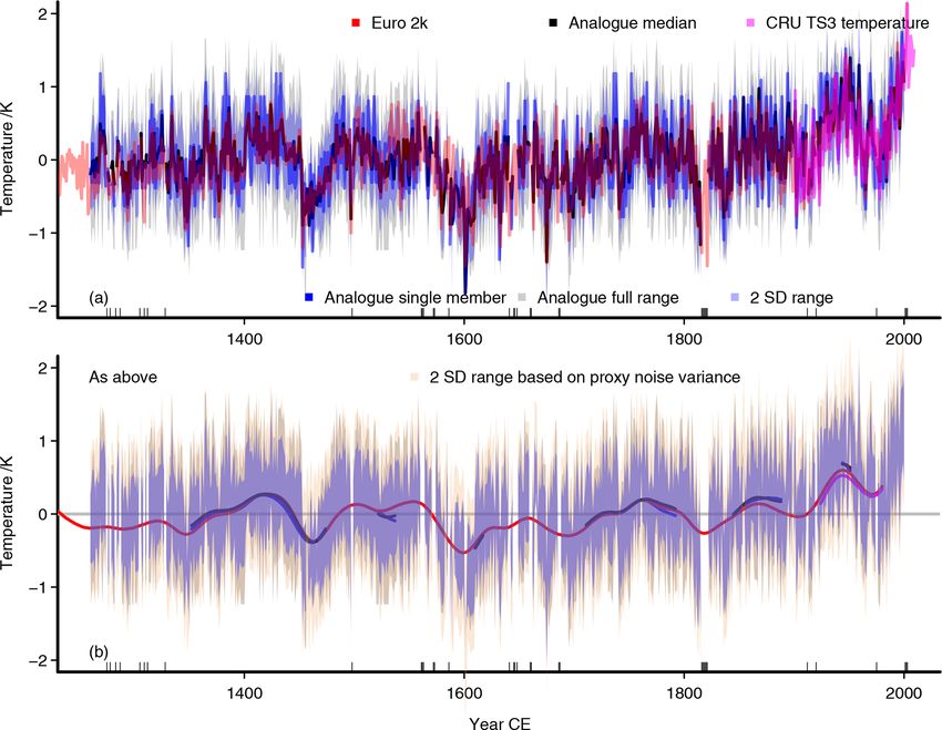
346                                                   O. Bothe and E. Zorita: Uncertainty of proxy surrogate reconstructions

construction effort. That is, we, as Luterbacher et al. (2016),   Table 3. Simulations in our pool of analogue candidates: ID, forc-
exclude these proxies because there is not a clear relation to    ing components, data reference. We consider for all eight simu-
temperature. Furthermore, since the Dobrovolný et al. (2010)      lations the period of 800 to 2005 CE, i.e., 1206 simulated years.
central European data are a spatial average, we also do not       Forcings are stratospheric sulfate aerosols from volcanic eruptions
consider them in the reconstruction. The central European         (V), variations of total solar irradiance (large amplitude: S, small
                                                                  amplitude: s), changes in Earth’s orbit (O), land use change (L),
data are subsequently compared to the reconstructed data.
                                                                  greenhouse gases (G); note, only methane and nitrous oxide were
   We describe results for the period of 1260 to 2003 CE, al-     prescribed; the carbon dioxide concentration was calculated inter-
though two of the Euro 2k proxy series extend back to the         actively. For details, see data references and Jungclaus et al. (2010).
year 138 BC, and the analogue approach is suited to use vari-
able numbers of proxies. The latest start date of any of the               ID          Forcing     Reference
used eight proxy indices is the year 1260 CE, and thus all
eight records cover the period of 1260 to 2003 CE. We decide               mil0010     VsOLG       Jungclaus (2008a)
against using uneven numbers of proxies and against extend-                mil0012     VsOLG       Jungclaus (2008b)
                                                                           mil0013     VsOLG       Jungclaus (2008c)
ing the reconstruction further back to ease the comparison of
                                                                           mil0014     VsOLG       Jungclaus (2008d)
the results and our different uncertainty estimates.                       mil0015     VsOLG       Jungclaus (2008e)
                                                                           mil0021     VSOLG       Jungclaus and Esch (2009)
2.2.2   Model simulations                                                  mil0025     VSOLG       Jungclaus (2009a)
                                                                           mil0026     VSOLG       Jungclaus (2009b)
Thanks to the PMIP3 effort (Paleoclimate Modelling Inter-
comparison Project phase 3, e.g., Schmidt et al., 2012), there
exists a multi-model ensemble of climate simulations for the
                                                                  ation over the same period. Jungclaus et al. (2010) provide
last approximately 1100 years. A number of additional simu-
                                                                  details on the simulations (see also data references in Ta-
lations comply with the PMIP3 protocol but are not included
                                                                  ble 3). We use simulation output from the ensemble mem-
in the effort (Jungclaus et al., 2010; Fernández-Donado et al.,
                                                                  bers including all forcing components for the period of 800
2013; Lohmann et al., 2015; Otto-Bliesner et al., 2016).
                                                                  to 2005 CE (Table 3). Thereby, we have a pool of 9648 can-
Wagner (Sebastian Wagner, personal communication, 2016,
                                                                  didate fields. Forcings are solar, volcanic, greenhouse gas,
2019) has performed a simulation for the last 2000 years,
                                                                  orbital, and land use; the carbon dioxide concentration was
and Gómez-Navarro et al. (2013, see also Gómez-Navarro
                                                                  calculated interactively (compare Jungclaus et al., 2010).
et al., 2015a) and Wagner (Sebastian Wagner, personal com-
munication, 2014, 2018, 2019; see also Bierstedt et al., 2016,
Bothe et al., 2019) has performed regional simulations for        3     Results
Europe for approximately the last 500 years. All these simu-
lations would be suitable as a pool of analogues. Especially      3.1    Single best-analogue reconstruction
the PMIP3 ensemble is easily available.
   We opt here for a single model ensemble predating the          Figures 2 and 3 compare the single best-analogue reconstruc-
PMIP3 effort but compliant with its protocol, i.e., the mil-      tion to the Euro 2k reconstruction and the observational data
lennium simulations with the COSMOS setup of the Max-             relative to the full period (1260 to 2003 CE). There is gener-
Planck-Institute Earth System Model (MPI-ESM) by Jung-            ally good agreement between the Euro 2k reconstruction and
claus et al. (2010). This choice is mostly based on the as-       the analogue reconstruction, but the latter appears to over-
sumption that the simulations provide a very similar inter-       estimate the warming starting from the early 19th century
nal variability. This is beneficial in our case because we        (Fig. 2a). Note that the observational data are plotted relative
rescale the final reconstructions by a chosen standard devi-      to the mean of the Euro 2k reconstruction over the observa-
ation, which is usually the local full-period standard devia-     tional period and solely provide a qualitative comparison. We
tion of one of the simulations. Furthermore, one may assume       evaluate our analogue reconstruction against the Euro 2k re-
that the single model ensemble provides data with a consis-       construction, because we regard the former reconstruction as
tent bias throughout the ensemble, which may ease compar-         the main benchmark for the analogue uncertainty estimation.
ison of the results. On the other hand, such consistent bi-       Figure A1 in the Appendix makes the comparison relative to
ases may translate to the reconstruction, i.e., a biased recon-   the period of the observational data. We note that differences
struction. This could be avoided by using a pool of simula-       between the observations and the reconstructions are larger
tions from structurally different climate models. Obviously,      for the best-analogue approach compared to the Euro 2k re-
the shortcomings in simulating the El Niño–Southern Oscil-        construction (Figs. 3a and A2).
lation (ENSO) (Jungclaus et al., 2006) are prominent in the          The analogue reconstruction shows rather small centennial
MPI-ESM-COSMOS ensemble and affect the results.                   variations as does the Euro 2k reconstruction (Fig. 2). We
   We use data centered on the full period of 1260 to             note that the Bayesian hierarchical modeling (BHM) recon-
2003 CE, and the data are normalized with the standard devi-      struction by Luterbacher et al. (2016) shows larger variations

Clim. Past, 16, 341–369, 2020                                                                    www.clim-past.net/16/341/2020/
O. Bothe and E. Zorita: Uncertainty of proxy surrogate reconstructions                                                                     347

Figure 2. The best-analogue reconstruction relative to its full-period mean: (a) the interannual temperature reconstruction in black, the red
line is the area mean Euro 2k reconstruction, magenta is the observational CRU temperature adjusted to the mean of the reconstruction over
its time range. The analogue reconstruction is rescaled by the variability from one of the simulations. Panel (b) is the same as (a) but for 47-
point Hamming filtered data; we further add the uncertainty estimates for the interannual data: red is the unsmoothed Euro 2k uncertainty, the
blue envelope is a 2 standard deviation uncertainty based on the correlation between the proxies and the observations at the proxy locations,
the grey envelope is a 2 standard deviation uncertainty based on a mean squared error (MSE) estimate. Panel (b) adds a zero line as visual
assistance.

compared to their composite-plus-scaling reconstruction in                servational data emphasize that the analogue reconstruction
the early part of the last millennium prior to our study period.          (magenta dots in Fig. 3a) disagrees more with the observa-
The larger warming starting from about 1800 in the analogue               tions than the Euro 2k reconstruction does (red dots).
reconstruction is in line with a slightly larger warming in the              Considering uncertainties for the reconstructions, Fig. 2b
BHM reconstruction by Luterbacher et al. (2016). Figure A3                shows the unsmoothed 2 standard deviation uncertainties for
in the Appendix shows a comparison of the best-analogue                   the Euro 2k reconstruction and the single best-analogue re-
reconstruction to the two European summer temperature re-                 construction together with the smoothed records. We show
constructions of Luterbacher et al. (2016). This complements              two uncertainty estimates for the analogue reconstruction as
Fig. 2, where we show the comparison to the Euro 2k recon-                described in Sect. 2.1. The Euro 2k uncertainty intervals in
struction of PAGES 2k Consortium (2013a).                                 Fig. 2b are derived from the data provided by the PAGES 2k
   Figure 3a shows differences between different datasets as              Consortium (2013a), and they are based on the range of a
swarm plots. Swarm plots are categorical scatter plots, where             nested composite-plus-scaling reconstruction ensemble and
the data points are adjusted to avoid overlap between points.             the standard deviation of the reconstruction-validation resid-
Thereby, swarm plots provide information on the distribu-                 uals (see the Supplement to PAGES 2k Consortium, 2013a).
tion of the data plotted. The differences between the Euro 2k                The noise-variance-based envelope for the best-analogue
composite-plus-scaling reconstruction and the best-analogue               reconstruction is generally wider than the uncertainty of the
reconstruction highlight again their reasonable agreement                 Euro 2k reconstruction, while the mean squared error (MSE)-
(Fig. 3a on the left in grey dots). These differences do not              based analogue uncertainty is usually narrower. The MSE-
exceed 1 K. Time series plots of the smoothed differences                 based uncertainty is also generally narrower than the noise-
reveal temporal structure with periods of over- and under-                based uncertainty but can become occasionally very wide.
estimation (not shown). Differences are especially large in               The latter widening reflects that the best analogues may fit
periods before the 1600s and starting from about 1800 (not                poorly to the proxy records. The MSE-based uncertainty es-
shown). Differences between the reconstructions and the ob-               timates become particularly wide in the late 20th century,

www.clim-past.net/16/341/2020/                                                                             Clim. Past, 16, 341–369, 2020

348                                                        O. Bothe and E. Zorita: Uncertainty of proxy surrogate reconstructions

Figure 3. Further information about the single best-analogue reconstruction: (a) swarm plots for the differences between different datasets
relative to their periods of overlap: grey is the Euro 2k reconstruction minus the single best analogue, red is the CRU TS data minus the Euro
2k reconstruction, and magenta is the CRU TS data minus the single best analogue. Since the data are relative to their overlapping period, the
visualization hides potential biases. (b) Ratio between the standard deviations of the normalized analogue values at the closest grid points to
the normalized proxy values. (c) Mean squared error between the normalized analogue grid-point values and the normalized proxies, i.e., the
basis for one of the uncertainty estimates in Fig. 2. Swarm plots are categorical scatter plots that ensure that points do not overlap.

highlighting that the single best analogues found for this pe-            the MSE-based uncertainty estimate. Figure 4 plots both the
riod do not match the proxy data well. The best-analogue re-              proxy values as squares and the best-analogue values at the
construction is generally within the 2 standard deviation un-             closest grid points as lines for years of interest and arbitrar-
certainty of the Euro 2k reconstruction. Similarly, the noise-            ily selected years. The analogues agree well with the proxies,
based uncertainty estimate for the analogue reconstruction                e.g., for the year 1827, but notable differences occur as well,
usually includes the Euro 2k data.                                        e.g., for the years 1601 or 2002. Overall, this small selection
   Both uncertainty measures for the analogue reconstruction              indicates that the considered simulation ensemble represents
describe different but not mutually exclusive parts of the un-            well the relation between the considered regions. We note
certainty of the reconstruction. The variance-based envelope              that for these years and the selected analogues, it is not nec-
estimates the reconstruction uncertainty based on the local               essarily the case that spatial clustering of proxies in the Alps
agreement between proxies and observations over the period                or Scandinavia results in close agreement.
when instrumental data are available. Thus, it is unlikely that              A slightly disconcerting feature is visible for, e.g., the year
the uncertainty of the reconstruction at any time is smaller              1947, where the analogue appears to underestimate the intra-
than this estimate because we can assume that the quality                 location variability. Figure 3b shows the relation between
of the proxies is best in the recent period. The proxy-based              the standard deviation of the best-analogue locations and
noise uncertainty estimate includes local information but ex-             the standard deviation of the proxy records as swarm plots.
trapolates this over the period without instrumental data. On             While the intra-grid-point variability can be larger than the
the other hand, the mean square error captures the misfit be-             intra-proxy variation, it is apparent that the ratio is more of-
tween the uncertain proxies and the final reconstruction prod-            ten smaller than 1, indicating that the intra-proxy variation is
uct. Where it is smaller than the variance-based estimate, we             larger.
would call it unrealistic. When it exceeds this estimate, it is              Figure 3c adds the mean squared error of the best-analogue
preferable.                                                               locations and the proxy values. As already seen in Fig. 2,
   Both measures of reconstruction uncertainty rely on the                for the MSE-based uncertainty envelope, the errors are of-
level of agreement between reconstructed and observed data.               ten rather small, but there are times when they become very
In the following, we particularly look at the agreement be-               large. This stresses again that the best analogue may occa-
tween the reconstructed data and the proxy data as it enters              sionally fit the proxies rather badly.

Clim. Past, 16, 341–369, 2020                                                                           www.clim-past.net/16/341/2020/
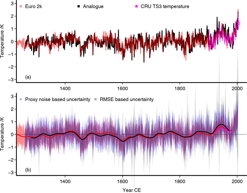
O. Bothe and E. Zorita: Uncertainty of proxy surrogate reconstructions                                                                 349

Figure 4. Normalized proxy values (squares) for proxies included and the values of the best analogue for selected years (lines). Proxy loca-
tions on the x axes are from PAGES 2k Consortium (2013a): Tor (Torneträsk, Sweden), Jae (Jämtland, Sweden), Nsc (northern Scandinavia),
Car (Carpathians, Romania), Aus (Alps, Austria), Swi (Alps, Switzerland), Fra (Alps, France), Pyr (Pyrenees, Spain).

   We do not investigate the differences in intra-location vari-        tainty estimates for the single best-analogue reconstruction.
ability in detail. There are a number of explanations on which          The potential of the MSE-based uncertainties to become very
we only very shortly touch here. First, the noisy proxy se-             large emphasizes that a best analogue may be a very bad fit
ries may overestimate the true intra-location variability. Sec-         for the underlying proxies. Indeed, uncertainty levels gen-
ond, our selected simulations may be spatially too smooth.              erally include the other reconstruction, which helps to build
This, thirdly, might be due to the low resolution, and sim-             confidence in the estimates. We regard this convergence of
ulations with higher resolutions might help then. Fourth, the           evidence important for confidence in our understanding of
chosen distance measure may result in such a feature depend-            past climates. Strong differences with the central European
ing on the characteristics of the simulation pool, which how-           data (e.g., Fig. 5) challenge how well the included proxies
ever should usually not be the case. Including a more diverse           really represent the European domain and its intra-regional
set of simulations may be the simplest way to investigate this          relations.
in future applications.
   Figure 5 provides a summary evaluation of the local dif-
ferences by showing swarm plots for the various proxy loca-             3.2    A set of “good” analogues
tions. The figure also gives the correlations between the prox-         As described above, we also consider a reconstruction based
ies and the local records from the analogues. Differences are           on a set of good analogues. One could base such a selection
well constrained for the proxies included but become very               on an arbitrary number of, e.g., 10 analogues. However, we
large for the area mean central European record. Indeed, cor-           base our choice of the number of analogues on our consid-
relations are also small for this record, while generally being         erations in Sect. 2.1.2 on the uncertainty of the local proxies
larger than 0.85 for the included records. The swarm plots              and on the number of analogues available for different uncer-
hide low-frequency variations in the differences for some of            tainty levels of the proxies. That is, in our case, a 2.57 SDnoi
the proxies (not shown). For example, the Swiss Alps data               uncertainty interval for the proxy values allows for at least
show a small amplitude multicentennial variation in their lo-           39 analogues for each date. Thus, we select 39 analogues at
cal differences.                                                        the locations of the grid points closest to the proxy locations.
   In summarizing, the general agreement between the Euro                  Figure 6 presents local results for the analogue search re-
2k and the analogue reconstruction as seen in Fig. 2 and                construction for the case of a fixed number of analogues. We
this section is another encouraging sign that the analogue              display the correlation coefficients between the proxies and
method is a valid reconstruction tool at least for the con-             the reconstructed local series medians at the top of each panel
sidered time period and regional focus. We give two uncer-              next to the proxy ID. They are between 0.84 and 0.98 for the

www.clim-past.net/16/341/2020/                                                                          Clim. Past, 16, 341–369, 2020

350                                                        O. Bothe and E. Zorita: Uncertainty of proxy surrogate reconstructions

Figure 5. Differences between local grid-point series for the single best analogue and the proxy series as swarm plots. Numbers above the
x axis are correlation coefficients between the proxy series and the grid-point records. Proxies are Torneträsk (Tor), Jämtland (Jae), northern
Scandinavia (Nsc), Carpathians (Car), Austrian Alps (Aus), Swiss Alps (Swi), French Alps (Fra), and the Pyrenees (Pyr). Ceu is central
European data. All data are from the normalized series and thus dimensionless.

Figure 6. Analogue reconstruction values at the locations of the included proxies. Shown are the normalized proxies in red, the median of
39 analogue values in black, and the full range of the 39 local analogues in blue. The x axes are years CE. Correlations between the local
reconstruction median and the proxy series are given as numbers next to the proxy IDs in each panel.

anchor locations of the reconstruction. These correlation co-             closely with the simulated data. Thus, successful constraints
efficients are larger than the correlations to the observational          provide confidence in the method but tell little about past cli-
data. That is, the proxies included in our analogue search                mate. We stress that the correlations only indicate agreement
constrain the search effectively towards the proxy values.                with the proxy records and not with the true temperature.
This holds especially for the median, which is a filter for the              The good agreement between the proxies included in our
data of the reconstruction ensemble members. The aim of the               analogue search and our reconstructed local series extends
analogue search is to match the observations, i.e., the proxies,          beyond correlations. The range of reconstructed values usu-

Clim. Past, 16, 341–369, 2020                                                                           www.clim-past.net/16/341/2020/
O. Bothe and E. Zorita: Uncertainty of proxy surrogate reconstructions                                                        351

ally is narrow for these proxies. However, there are also ob-      chor the area mean reconstruction to a narrow range of vari-
vious mismatches, e.g., 16th century warmth in the Austrian        ability if we choose a fixed number of analogues.
Alps and, more frequently, individual very cold excursions,           The distribution of the uncertainty estimates of the 39-
which are not matched in the analogues (Fig. 6). Plotting          analogue median is narrower than for the single best ana-
local analogue data against the proxy series highlights how        logue, and the distribution also has smaller values than for the
commonly the reconstruction median and random individual           two estimates for the single best analogue. However, in this
analogue members do not match the extreme values of the            case, the variability of the fixed number of analogues does
proxies (not shown). These considerations highlight that, al-      not encompass the full range of potential analogues com-
though the analogues may be well constrained locally, this         pliant with a specific uncertainty level. Again, we note that
gives no indication about the strength of the relations away       as long as an uncertainty estimate is smaller than the proxy
from the anchoring locations. Indeed, correlations with the        noise-based estimate as seen in Fig. 2, we think one should
observational CRU data are in line with the correlations be-       use the proxy noise-based uncertainty.
tween the proxies and the CRU data (not shown). Section 3.7           Interannual differences between the single best-analogue
shows that, indeed, the correlations in Fig. 6 do not necessar-    reconstruction and the median of the 39-analogue recon-
ily reflect how well the reconstruction captures the observed      struction appear to be of similar size as the interannual dif-
temperature elsewhere.                                             ferences between the Euro 2k reconstruction and the 39-
   Figure 6i shows the comparison for the spatial average          analogue median (not shown). The smoothed representations
summer temperature for the central European area (Dobro-           align quite well for the two different analogue approaches.
volný et al., 2010). This mean is computed over the grid           On the other hand, there are some systematic differences be-
points from 7.5 to 18.75◦ E and 46.4 to 50.1◦ N in the coarse-     tween the 39-analogue median and the Euro 2k reconstruc-
resolution model data. This domain obviously represents a          tion in the smoothed version particularly in the 14th and 16th
larger area than the data by Dobrovolný et al. (2010). There       centuries and starting from approximately the year 1850. We
is not any identifiable variability in the uncertainty envelope.   generally assume that such systematic differences are due to
Consequently, the median also shows very little variability.       differing sensitivities between the regression-based approach
Nevertheless, the variability is comparable between central        of the Euro 2k reconstruction and our analogue search. How-
European data for the analogue reconstruction and the orig-        ever, considering the mid-16th century, the work by Wetter
inal record if one considers individual members. Although          and Pfister (2011, 2013) may suggest that indeed our simula-
the temporal variations of the median are muted, the median        tion pool is insufficient for this period and the Euro 2k data
record still correlates notably but not strongly with the cen-     more reliably capture the temperature then.
tral European data of Dobrovolný et al. (2010).                       Differences between the two analogue approaches do not
   The median of the fixed-number analogue ensemble is             show such systematic differences except maybe for the early
shown in Fig. 7. It correlates slightly better with the Euro       20th century. Both analogue approaches appear to overesti-
2k reconstruction at r ≈ 0.89 than the single best analogue        mate the warming trend since the early 19th century. This
(r ≈ 0.82). The variability of the median of the analogues,        is more pronounced in the single best reconstruction com-
however, is approximately 8 % smaller than the variability of      pared to the median of the 39 analogues, for which we al-
the Euro 2k reconstruction and approximately 17 % smaller          ready noted the reduced variability.
than the variability of the single best-analogue reconstruc-
tion. Similarly, while the range of the best analogue is com-
parable to the Euro 2k reconstruction, the range of the 39-        3.3   Analogues within 1 SDnoi
analogue ensemble median is strongly reduced compared to
both other series. The coldest values are only slightly warmer     The use of a fixed number of analogues in the previous
but the warmest values are about 1 K colder than for the           section implies that we consider for each date a different
other two series. Therefore, using a set of analogues to pro-      level of proxy uncertainty according to our considerations
duce a reconstruction suppresses variability. This reduction       in Sect. 2.1.2. Next, we shortly present a reconstruction for
of variability for median- or mean-based reconstructions is        which we consider only those analogues falling within a cer-
expected due to the compensation of noise and within the in-       tain uncertainty interval around all of the original proxies for
dividual members. It is well established that such a trade-off     each date. This will result in an uneven number of analogues
between accuracy and variability exists for analogue search        at each individual date. We use a fixed 1 noise standard devi-
algorithms (Gómez-Navarro et al., 2015b, 2017).                    ation interval around the proxy values. The method is more
   Although the uncertainty of the regional average for cen-       likely to find valid analogue for all dates if we choose larger
tral Europe shows a wide uncertainty for the 39 analogues,         uncertainty intervals. However, larger intervals imply that the
the full domain reconstruction has a rather narrow uncer-          number of analogues may become exceedingly large for cer-
tainty range. The full ensemble range and a 2 standard de-         tain dates. As mentioned above, the 1 standard deviation in-
viation uncertainty based on the variance of the ensemble are      terval has a maximal number of 2105 possible analogues,
nearly indistinguishable in Fig. 7. The included proxies an-       which one may already rate as too many.

www.clim-past.net/16/341/2020/                                                                   Clim. Past, 16, 341–369, 2020
352                                                       O. Bothe and E. Zorita: Uncertainty of proxy surrogate reconstructions

Figure 7. The analogue reconstruction for the 39 best analogues. (a) The interannual rescaled temperature reconstruction median in black;
the blue line is the single best-analogue reconstruction; the red line is the Euro 2k reconstruction; magenta is the CRU temperature adjusted
to the mean of the reconstruction median over the CRU period. (b) The unsmoothed uncertainty, estimates given by light grey lines are
the ensemble range, and the brown envelope gives a 2 standard deviation interval based on the variance of the 39 samples; note that both
uncertainty estimates are nearly indistinguishable on this scale, the panel adds the series from (a) but for 47-point Hamming filtered data.
Panel (b) adds a zero line as visual assistance.

   Figure 8 displays the results for such an analogue recon-             COSMOS millennium simulation ensemble includes ana-
struction collecting all analogues within 1 noise standard de-           logues also matching the recent summers. However, we do
viation around the proxy values. Again, there is good agree-             not search analogues that only fit the observed area mean
ment between the analogue reconstruction and the Euro 2k                 warming regionally or globally, but we search for analogues
reconstruction. Blue lines in Fig. 8a show a single member               that also represent the interrelation among the proxy loca-
of the reconstruction ensemble which also compares quite                 tions and do so within a fixed noise threshold. Under these
well to the Euro 2k reconstruction.                                      constraints, it is considerably harder to find analogues. The
   As indicated before, if one chooses smaller uncertainty in-           European temperature slowly leaves the temperature range
tervals around the proxy values, it becomes more likely that             observed in approximately the previous 750 years, and we
the method fails to identify suitable analogues. This becomes            have only few candidate fields that may represent the warm
obvious when considering the smoothed estimates. This way                climate after the year 2000 CE, e.g., the summer heat of the
of constraining the analogue space quite frequently fails to             year 2003 CE (compare, e.g., Wetter and Pfister, 2013; Black
provide any analogue at all. Small ticks at the time axes of             et al., 2004; Stott et al., 2004; Garcia-Herrera et al., 2010).
Fig. 8 show that such failures appear to cluster in the 13th             Additional gaps occur in uncertainty envelopes based on the
and 14th centuries, in the 16th and 17th centuries, and in the           ensemble variance when there is only one valid analogue.
early 19th century. A number of these are years with strong                 Figure 8 shows three different uncertainty estimates. For
forcing from volcanic eruptions (compare Sigl et al., 2015).             one, there is in both panels in grey the full range of the
This is a shortcoming of our approach to uncertainty in this             analogues that comply with the 1 noise standard deviation
section. Our results in previous sections as well as subsam-             around the proxy values. Second, the panels show in blue a
pling approaches (e.g., Neukom et al., 2019) do not have this            2 standard deviation uncertainty based on the variance of the
specific problem.                                                        ensemble members at each date. The latter is in this case usu-
   Another period without suitable analogues occurs after the            ally notably narrower than the full range, which reflects to a
year 2000 CE. Considering the results of Jungclaus et al.                good part simply the number of available analogues. We also
(2010, e.g., their Fig. 3), one might have hoped that the                add in Fig. 8b an assumed 2 standard deviation uncertainty

Clim. Past, 16, 341–369, 2020                                                                          www.clim-past.net/16/341/2020/
O. Bothe and E. Zorita: Uncertainty of proxy surrogate reconstructions 353
Figure 8. Analogue reconstruction based on an 1 SDnoi uncertainty of the proxies. (a) Interannual data: red, the Euro 2k reconstruction;
black, the analogue median; blue line, a single analogue member; blue shading, 2 standard deviation uncertainty range around the analogue
median based on variability of the analogues; grey shading, the full range of analogues; marks at horizontal axis mark unsuccessful analogue
searches. Panel (b) is the same as (a) for 47-point Hamming filtered data, but we add a 2 standard deviation uncertainty based on the square
root of the proxy noise variances in brown, as also shown in Fig. 2. Panel (b) adds a zero line as visual assistance.
envelope based on the proxy noise at each individual proxy The 24 analogues for the year 1424 have a tendency to-
location. It is slightly wider than the full range of the ensem- wards warm values, but again warm and cold conditions are
ble. found within a 1 standard deviation interval around our proxy
Until now, we concentrated on time series. Figure 9 shows anchors for southeastern and southwestern Europe. On the
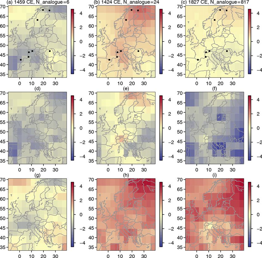
how the analogue reconstruction can provide diverse spatial other hand, the six analogues available for the year 1459
representations for the same set of proxy values. It can give mostly give slightly cold conditions over wide parts of the
several different reconstructions that strongly differ from domain and especially for continental Europe.
each other. The example years are chosen to represent a Figure 10 reflects on the potentially very wide local range
rather cold, a rather warm, and an approximately average of the analogues. It shows the mean range and the maximum
year, and the top row shows the median of the found ana- range of the ensembles for the field. Thereby, it summarizes
logues for the three cases of 1459 CE, 1424 CE, and 1827 CE. the local uncertainties for the analogue fields. Dependent on
Incidentally, these are also three years for which we find few, location, the mean range of the ensemble is between approx-
i.e., 6, reasonable, i.e. 24, and as many as 817 analogues imately 1.7 K and approximately 5.9 K (Fig. 10a). The mean
in a 1 standard deviation interval. The subsequent rows add range is generally large at the eastern border of the domain,
the local minimum and maximum values, respectively. Black and it becomes also large over the southern Adriatic Sea, the
dots in the top row show the original proxy locations. Note central Baltic Sea, and particularly at the western boundary
that the figure displays temperature anomalies from the mean over the Iberian Peninsula. The local maxima of ranges over
over the full period in Kelvin. time mirror the distribution of the mean ranges. Further, they
It is surprising that, e.g., the proxies anchor the year 1827 emphasize how weakly constrained the reconstructions are
in Turkey only within a range of up to 8 K for the more than throughout the domain (Fig. 10b).
800 analogues. Even central Scandinavia may be rather cold We noted for Fig. 4 that it is not necessarily the case lo-
or rather warm, although it should be constrained by three cally that individual analogues fit better in regions with mul-
proxy records. Indeed, the best analogue for that year is close tiple proxies. However, the mean ranges in Fig. 10 are indeed
to the proxies (compare Fig. 4). smallest in northern Scandinavia and the Alps, and small
ranges extend towards the French coast of the Mediterranean.
www.clim-past.net/16/341/2020/ Clim. Past, 16, 341–369, 2020You can also read