New Vehicle Fuel Economy and CO2 Emission Standards Emissions Evaluation Guide - Francisco Posada, Zifei Yang & Kate Blumberg International ...
←
→
Page content transcription
If your browser does not render page correctly, please read the page content below

New Vehicle Fuel Economy and
CO2 Emission Standards
Emissions Evaluation Guide

Francisco Posada, Zifei Yang & Kate Blumberg
International Council on Clean Transportation – ICCT

Project Context The Guide
The Advancing Transport Climate Strategies (TraCS) project is im- This guide on the calculation of emissions baselines of new vehicle
plemented by the Deutsche Gesellschaft für Internationale fuel economy and CO2 emission standards was developed by the
Zusammenarbeit (GIZ) and funded through the International
International Council for Clean Transportation (ICCT) together
Climate Initiative of the German Ministry for the Environment, with a Microsoft Excel based spreadsheet tool – the Fuel Economy
Nature Conservation, Building and Nuclear Safety (BMUB). Standards Evaluation Tool (FESET). FESET includes data of the
Its objective is to enable policy makers in partner countries Mexican new vehicle CO2 emissions and fuel economy standards
(Vietnam and Kenya) to specify the con-tribution of the transport for 2012 to 2016, as an example. The tool is open so that values can
sector to their respective Nationally Determined Contributions be exchanged and adapted to allow applying the tool in other
(NDCs). Detailed knowledge on transport-related emissions and countries, too. Chapter 6 provides a step-by-step description of the
mitigation potentials can furthermore lead to raising the level of Mexican example and how to apply the FESET.
ambition in the two countries.
The project follows a multi-level approach:
At the country level, TraCS supports (transport) ministries and
other relevant authorities in systematically assessing GHG emissi-
ons in the transport sector and calculating emission r eduction po-
tentials through the development of scenarios.
At the international level, TraCS organises exchanges between im-
plementing partners, technical experts, and donor organisations to
enhance methodological coherence in emission quantification in
the transport sector (South-South and South-North dialogue). The
dialogue aims to increase international transparency regarding
emissions mitigation potential and the harmonisation of methodo-
logical approaches in the transport sector. As part of this internati-
onal dialogue, TraCS also develops knowledge products on emissi-
ons accounting methodologies.
New Vehicle Fuel Economy and CO2 Emission Standards Emissions Evaluation Guide 3
Content

        Project Context / The Guide                                                                                             03

        1. Description and characteristics of fuel economy standards for light-duty vehicles                                    05

        2. Structure of mitigation effects                                                                                      08

          2.1 Cause impact chain                                                                                                08

          2.2 Key variables to be monitored                                                                                     09

          2.3 Interaction factors                                                                                               11

          2.4 Boundary setting                                                                                                  12

          2.5 Key methodological issues                                                                                         14

          2.6 FE/GHG standard complementary policies                                                                            16

        3. Determining the baseline and calculating emission reductions                                                         17

          3.1 Analysis approach                                                                                                 17

          3.1.1 Determination of baseline new-vehicle fleet-average GHG emissions                                               17

          3.1.2 Fleetwide GHG emission model development                                                                        18

          3.2 Uncertainties and sensitivity analysis                                                                            22

        4. Guidance on the selection of analysis tools for new vehicle GHG and fuel economy standards for light-duty vehicles   23

          4.1 Description of tool types                                                                                         24

        5. Monitoring                                                                                                           26

        6. Example – Impact of new vehicle CO2 Standards in Mexico                                                              29

        References                                                                                                              36

        Imprint                                                                                                                 37

4    New Vehicle Fuel Economy and CO2 Emission Standards Emissions Evaluation Guide
1. Description and characteristics of fuel economy standards
for light-duty vehicles
Fuel economy (FE) or greenhouse gas (GHG) emission standards Globally, the application of stringent GHG/FE standards in key
regulations are one of the main instruments available to policy regions is expected to attenuate and even offset growth in vehicle
makers to achieve significant improvements in fuel consumption activity and vehicle sales numbers by reducing overall GHG
and GHG emissions from light-duty vehicles (LDVs). These emissions from the transportation sector. Figure 1 shows the evolu-
standards require new LDVs to achieve lower fuel consumption tion of sales weighted carbon dioxide (CO2) emissions from the
and GHG emissions over time through continued development passenger car fleets of ten countries with GHG or FE standards in
and application of fuel efficient technologies. Adoption of such place today (Yang, 2017). The figure compares country standards
standards results in a market transformation towards vehicles that for passenger vehicles in terms of grams of CO2-equivalent per
are increasingly fuel-efficient-consuming less fuel per kilometre kilometer adjusted to the European NEDC test cycle. The
driven and thus emitting less GHG. European Union has historically outpaced the world with the
lowest fleet average target of 95 gCO2/km by 2021. However,
New GHG emission and FE standards regulations are policies South Korea will match, if not exceed the European Union with a
typically set at the national level and typically span three to eight fleet target of 97 gCO2/km in 2020. With high hybrid percentage,
years. Additional regulatory phases are commonly applied to Japan already reached its 2015 target of 142 g/km in 2011 and
continue these policies. Successful implementation of new vehicle 2020 target of 122 g/km in 2013. If Japan keeps reducing CO2
GHG/FE standards translates into more efficient vehicles being emissions at this same rate, Japan’s passenger vehicle fleet would
incorporated into the fleet, which, combined with the natural achieve 82 g/km in 2020, far below the targets set by other coun-
retirement of older and less efficient models, results in an impro- tries. The United States and Canada, long laggard in regulating fuel
vement of the national fleet average fuel efficiency. economy, have evolved into leaders. As the first country with 2025
targets, the example set by U.S. has encouraged other countries
The regulated entities are vehicle manufacturers and importers of (e.g., Canada) to consider enacting similarly long-term standards.
all new vehicles intended for sale within the country. Each automo- The United States is expected to achieve the greatest absolute GHG
tive manufacturer should meet a target value based on the LDV emission reduction – 49% – from 2010 to 2025. 1
fleet that it sells. Each manufacturer’s compliance with their target
ensures that the entire national fleet of new vehicles achieves the
desired reductions in GHG emissions and fuel use. FE/GHG
standards mandate no specific technology, fuel, or vehicle type/size.
Manufacturers can choose the technology pathway that is most sui-
table to their business plan while respecting local consumer
preferences.
1
China proposed a fleet average fuel consumption of 4 L/100km by 2025 (MIIT, 2015), which would be among the lowest target levels if it is enacted.
New Vehicle Fuel Economy and CO2 Emission Standards Emissions Evaluation Guide 5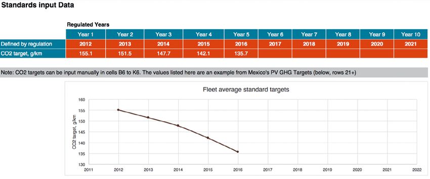
Figure 1: Passenger car sales CO2 emission targets and sales-weighted averaged actual fleet historical performance 2
Figure 2 presents an example of the overall impact of FE/CO2 jectives of the G20 Energy Efficiency Leading Program (EELP):
s tandards adoption for light-duty vehicles in selected G20 countries these aspirational targets include a 50% reduction in LDV fuel
(Miller, Du, and Kodjak, 2017). Three scenarios are compared for consumption compared to a 2005 base year by 2030 (G20, 2016).
new vehicle efficiency and CO2 standards: the “baseline” scenario The analysis by Miller, Du and Kodjak show that currently adopted
assumes no further improvements in new vehicle efficiency after vehicle efficiency standards will avoid 1.7 billion tons of carbon
2005, to enable the estimation of benefits from a dopted policies. dioxide (GtCO2) in 2040, whereas new world-class LDV efficiency
The “adopted policies” scenario includes all policies adopted as of standards could mitigate direct emissions from fuel combustion by
September 2016, including those taking effect in the future. Final- an additional 1.2 GtCO2 in 2040.
ly, the “world-class” scenario models the impacts of all countries
developing new vehicle efficiency standards consistent with the ob-
2
International Council on Clean Transportation (ICCT) 2016. Global PV Standard Library. Available at: http://www.theicct.org/global-pv-standards-chart-library
6 New Vehicle Fuel Economy and CO2 Emission Standards Emissions Evaluation Guide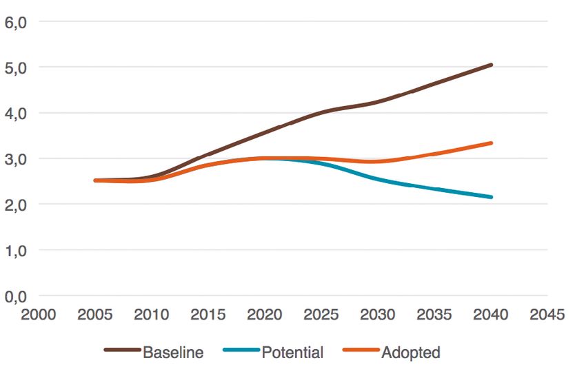
Figure 2 Direct combustion CO2 emissions of light-duty vehicles in selected G20 member states under baseline, adopted policies, and world-class
efficiency scenarios, 2005–2040.
Figure shows historical and projected emissions for Australia, Brazil, Canada, China, the EU-28 (including United Kingdom), India, Japan, Mexico,
the United States, and Russia. Source: Miller, Du, and Kodjak (2017)
Direct combustion Co2, Gt
Vehicle fuel economy and equivalent metrics
Different metrics can be used to describe the amount of fuel, HG/CO2 emissions measures GHG or CO2 emissions per distance
energy and GHG emissions generated by unit of distance traveled, expressed as grams of pollutant per kilometer or mile.
traveled by a vehicle. Selection of the metric is driven by the The metric can be expressed in grams of CO2 or CO2-equivalent
intention of the policy to either reduce fuel use, or GHG per unit distance (gCO2/km or gCO2e/km). A CO2-equivalent
emissions. (CO2e) metric incorporates emissions of non-CO2 pollutants,
using the global warming potential (GWP) to translate their im-
Fuel economy (FE) measures distance traveled per unit of fuel pact to CO2 equivalency. Primary GHGs besides CO2 are methane
consumed. The most common metrics are kilometers per liter (CH4), nitrous oxide (N2O), and fluorinated gases (F-gases).
(km/L) and miles per gallon (mpg) in the U.S.
Energy consumption (EC) measures the energy consumed per
Fuel consumption (FC) is the reciprocal of fuel economy, and distance traveled, for example in megajoules per kilometer
measures fuel consumed per distance traveled. It is usually (MJ/km). Despite being a less common metric, it is relevant as
expressed in liters per 100 kilometers (L/100 km), and it is a fuel-neutral metric across different fuel types and vehicle
used in Europe, for example. technologies. Vehicle energy consumption is the metric used in
Brazil’s vehicle efficiency standards policy.
New Vehicle Fuel Economy and CO2 Emission Standards Emissions Evaluation Guide 7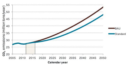
2. Structure of mitigation effects
2.1 Cause impact chain Adopting new vehicle GHG/FE standards regulations would pro-
vide the following direct and indirect benefits with respect to the
Adoption of new vehicle GHG/FE standards measurably reduces baseline scenario:
GHG emissions and fuel consumption for the average light-duty – Reduce the fleet average emission of CO2 and fuel consumed
vehicle via increased adoption of fuel efficient technologies. This per kilometer driven for the fleet covered.
improvement, coupled with new vehicle sales and activity–which – Reduce the total annual contribution of GHG emissions
have been showing significant growth in most emerging economies from the transportation sector.
(ORNL, 2016)–has the potential to significantly reduce fleetwide – Reduce fuel consumption from the transportation sector,
GHG emissions compared to business-as-usual (BAU) conditions. and, potentially, fuel imports.
Those reductions can be assessed applying bottom-up models – Reduce emissions of GHG and pollutants generated by oil
based on CO2 emission factors, number of vehicles, and vehicle extraction, fuel production, and distribution.
activity. This measurable fuel consumption and GHG reduction – Accelerate adoption of advanced efficiency technologies and
found in regulated average new vehicles would reduce the overall potentially incentivize transition to electric mobility and zero
vehicle fleet GHG impact as illustrated in Figure 3. emissions. As the standards become more stringent over time,
the most advanced fuel-efficient technologies are required.
Estimates by EPA in the US show that the most stringent
GHG/FE standards in 2025 would require increased adopti-
on of hybrid and battery electric vehicles to meet future stan-
dards (USEPA, 2016). Other complementary policy instru-
ments can be deployed to increase the rate of adoption via
direct taxation incentives or indirect incentives such as easier
access to high occupancy lanes or parking spots.
8 New Vehicle Fuel Economy and CO2 Emission Standards Emissions Evaluation Guide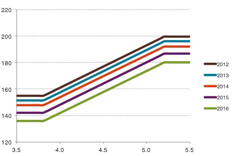
Figure 3 – Causal chain for new vehicle fuel economy and greenhouse gas emission standards

                                                                                                 Persons

                                                                                                 Trips/Person
                                                                                                                                    PKM
                                                                                                 Km/Trip

                                                                                                 Trips/Mode

                                                                                                 Load factor/Occupancy

                                                                                                 Number of veh./Type
                                                                                                                                    VKT
                                                                                                 Km/Vehicle type

            New light-
           duty vehicle
                                                                                                 Fuel/Km
             GHG/FE
            standards
                                                                                                                                          Fuel use

                                                                                                 GHG/Fuel

           Intended effect          Leakage/Rebound
                                                                                                                                                    GHG
                                                                                                                                                  emissions
           Historic and/or default values         Parameters to be monitored            Intermediate results

2.2 Key variables to be monitored                                                        Monitor for intended effects:
                                                                                         New Vehicle GHG or FE Standards
GHG/FE standards require vehicle manufacturers to achieve a                              Under a new vehicle GHG or FE standard, each automotive ma-
GHG emissions or fuel economy target level in a given year. Ap-                          nufacturer has a GHG/FE target value for its light-duty vehicle
plying the regulations to a reduced set of stakeholders rather than                      fleet sold into the market for a given year. Targets can be designed
individual consumers ensures compliance and simplifies enforce-                          in two ways: as manufacturer fleet average target values (also known
ment of the standards. Thus, the key variable to be monitored                            as corporate average) or as individual (per-vehicle) minimum effi-
when designing and implementing a new vehicle GHG/FE stan-                               ciency target values. 3 Fleet-average targets incentivize the manufac-
dard is the performance of each manufacturer with respect to its                         turer to offer very efficient models to balance out the less efficient
target. As GHG/FE standard targets become more stringent over                            ones. Fleet averaging offers flexibility to manufacturers to reach
time, monitoring is required on an annual basis. Other variables                         their respective targets, thereby facilitating setting strong targets.
that affect the actual GHG emissions of the transportation sector                        And because they provide an incentive for technology to keep im-
are new vehicle sales volume and vehicle activity.                                       proving, fleet-average targets ease the process of increasing standard

3
     s an example, the first two phases of the Chinese passenger car fuel consumption standards regulation (2005–2006 and 2008–2009) used a per-vehicle minimum efficiency
    A
    performance approach. The intention of the Ministry of Environmental Protection (MEP) was to force a quick phasing out of older vehicle technology. While this can be a
    useful approach for GHG/FE standards, this document is intended to support best practices to reduce fuel consumption and GHG emissions from new vehicles, and therefore
    the text focuses on a sales-weighted regulatory design.

                                                                 New Vehicle Fuel Economy and CO2 Emission Standards Emissions Evaluation Guide    9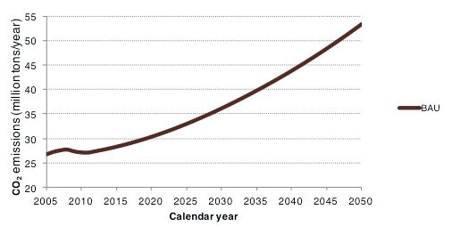
stringency over time. Per-vehicle minimum efficiency targets res- stringency of the target results in a fleet that becomes more efficient
trict the sale of models that have fuel consumption above some le- each year as new targets are set and new (more efficient) vehicles are
vel; they are restrictive to manufacturers but are easier to imple- phased in to meet them. While the new vehicle fleet average
ment and monitor. Due to the restrictive nature of this design, efficiency improves annually, older and less efficient vehicles are
per-vehicle targets are required to be less stringent compared to retired from the fleet, improving the overall vehicle stock fleet aver-
average targets to avoid imposing bans on a wide range of models. age fuel efficiency.
Such standards also offer a limited incentive for further investment
in efficiency technology development. Most countries with regula- An example comparison of the CO2 targets for Europe and the
ted vehicle fleets have adopted fleet average standards designs – as performance of each automotive manufacturer is shown in Figure
shown in Figure 1. Saudi Arabia’s FE program design is an interes- 4. The horizontal axis shows vehicle weight as the reference para-
ting example in that it applies fleet average targets for new vehicle meter and the vertical axis shows CO2 values. Lines show targets
sales and per vehicle maximum targets for its used import vehicle and dots show the actual CO2 performance of each manufacturer
sales (SASO, 2015). in 2015. The data for each manufacturer is based on a dataset pro-
vided by the European Environment Agency (EEA) that monitors
Each target is designed as a linear function of vehicle footprint 4 or CO2 emissions from new passenger cars in the EU (EEA, 2016).
vehicle weight, with less stringent targets for larger or heavier ve- The EEA data show that the mandatory emission reduction target
hicles. Using these metrics helps to specifically target vehicle effi- set by the EU legislation for 2015 was met on average. New cars
ciency technologies and avoid impacting consumer choices and sold in the EU in 2015 had average CO2 emissions of 119.6 g CO2
manufacturer competitiveness. The targets may be expressed in /km, which was 8% below the 2015 target, and 3% lower than in
grams of CO2 or CO2-equivalent per unit distance (gCO2/km or 2014. All major manufacturer groups met their mandatory CO2
gCO2e/km), distance driven per litre of fuel consumed (km/L), emission limits in 2015. For each manufacturer group, the 2020/21
energy per unit distance (MJ/km), or fuel consumed for certain target implies a decrease of approximately 27% in average CO2
distance (L/100km). emissions compared to the 2015 target (ICCT, 2016).
The targets are tightened over time. The rate of annual target im-
provement ranges between 3.5% to 6.0%. Annually increasing the
Figure 4 – Performance of the top selling EU passenger car manufacturer groups for 2015, along with 2015 and 2020/21 CO2 emission target lines.
Source: ICCT (2016)
180
160
2015
target line
140
Average CO2 emissions (g/km)
Fiat -27%
GM BMW
120 Ford Volkswagen
Daimler
Renault-Nissan Average
PSA Toyota
100
2020
target line
80
60
40
20
0
1100 1300 1500 1700
Average vehicle mass (kg)
4 The footprint of a vehicle is defined as the area circumscribed by the vehicle’s wheelbase and average track width (i.e., footprint equals wheelbase times average track width).
10 New Vehicle Fuel Economy and CO2 Emission Standards Emissions Evaluation GuideNumber of vehicles standard design or Monitoring & Reporting ex-ante and ex-post
The number of new vehicles entering the fleet each year (i.e., new activities, but it is recommended to observe official or academic
vehicle sales) is used as an input to calculate the total new vehicle publications for significant changes on fleet average VKT values.
fleet contribution to GHG emissions and fuel consumption. Indivi- VKT also changes with vehicle age; VKT degradation curves can
dual manufacturer new vehicle sales are also used as inputs to be d
eveloped to account for that, or can be adopted from similar
calculate performance with respect to the GHG/FE targets and to markets.
determine compliance with the standards. It should be noted that
new vehicle fuel economy standards do not regulate the number of One known negative indirect effect of new vehicle GHG/FE stan-
vehicles sold. dards for light-duty vehicles is the potential increase in vehicle
activity due to drivers experiencing lower fuel consumption and
Monitoring the current vehicle fleet size (or vehicle stock), via corresponding lower driving operating cost. This is known as re-
national vehicle registration data or other sources, is required to bound effect. The rebound effect for the transport sector has been
provide absolute GHG emissions and fuel consumption by the estimated to be between 3% and 18% for passenger vehicles in the
baseline fleet; it is also needed for calculating the relative impact of US (US EPA, 2015) and globally it has been estimated to be bet-
the intended action. Vehicle retirement rates are needed to estimate ween 10–30% for road transport (Lah, 2015; Fulton et al., 2013).
the outflow of vehicles from the vehicle stock and to provide an The numerical interpretation corresponds to that of an elasticity:
estimate of the current vehicle stock. Vehicle retirement rates are assuming a rebound effect of 10%, the impact of 25% impro-
mathematical functions that describe the probability of finding a vement in fuel efficiency would be a 2.5% increase in VKT (i.e.,
vehicle operating after certain age. A new vehicle is much more the 10% of 25%). The literature also concludes that the rebound
likely to be found operating (and contributing to the GHG inven- effect declines over time as population incomes rises (US EPA
tory) after year one of entering the fleet than a vehicle that entered 2015).
the fleet 30 years ago.
Vehicle activity 2.3 Interaction Factors
Vehicle activity, in kilometres traveled per vehicle per year or VKT,
is used as an input for calculating total fleet fuel consumption and The most important factors affecting the magnitude of the fuel
GHG emissions. Typically, the input comes as an average value by consumed and GHG emitted by the fleet are the design of the
vehicle type (e.g., light-duty, heavy-duty, urban buses, taxis) from GHG/FE standards, and the extent and activity of the vehicle fleet.
national statistical data from national road or transit authorities. Table 1 presents a summary of those factors and GHG effects.
This input does not require active monitoring as part of the
Table 1– Factors that affect key GHG/FE standards variables
Factor Changes Reasons for the change and effects on total GHG
GHG/FE regulatory design GHG target design and More stringent GHG targets with higher annual improvement rates
rate of annual impro- would result in lower total GHG emission reductions. Ambitious GHG
vement targets and annual rates of GHG improvement would have to be
evaluated against a realistic assessment of the ability of the regula-
ted party to achieve the targets via available technologies and costs.
Vehicle activity VKT changes due to Lower fuel operating costs due to more efficient vehicles may incen-
rebound effect tivize the consumer towards higher vehicle activity. This would off-
set to various degrees the reduction of total GHG emission from new
vehicle efficiency improvements.
Fleet size Increase in the number Rapidly growing vehicle markets will face more difficult challenges
of vehicles in the fleet reducing the total GHG emissions than more saturated markets, but
effective regulations will lead to bigger GHG reductions compare to
BAU.
GHG/FE Standards are not designed to affect vehicle sales. Other
policy instruments, such as vehicle taxes can have an impact on
fleet growth and replacement rates.
In regions where imports of used vehicles are significant compared
to new vehicle sales the impact of those vehicles on total GHG emis-
sions has to be estimated.
New Vehicle Fuel Economy and CO2 Emission Standards Emissions Evaluation Guide 112.4 Boundary setting For other vehicle types, such as heavy-duty vehicles, separate
GHG/FE standard regulations with different design elements
The boundary setting of MRV on GHG/FE standards is closely could be conceived. The regulation of heavy-duty vehicles, which
linked to the regulatory scope. GHG/FE standards are defined as span over a wider range of vehicle types, uses, and drive cycles (e.g.,
national or regional regulations. The technical scope of the regula- long-haul trucks, refuse trucks, delivery trucks), requires a very
tion calls for defining what type of vehicles would be covered under different approach and different technology packages are available
the standard and for how long. The regulatory target and the im- for different vehicle types and uses.
pacts on sustainability are also included as part of the boundary
definition. Ultimately, the decision on sectorial boundaries depends on the
country-specific vehicle class definitions as defined by national
Geographic boundary Ministries/Departments of Transport or Industry.
As a vehicle sale occurs at the national level, the geographic
boundary is at that level, under a national policy. It is acknowled- Time scale boundary
ged that local policy measures that complement national GHG/FE The temporal boundary of baseline determination for monitoring
standard regulations–in particular compact city planning and the and reporting should go beyond the regulatory implementation
provision of low-carbon transport modal alternatives, such as timeline. The regulatory implementation typically covers 3 to 8
public transport, walking, and cycling, are a vital component of a year periods, typically with the intent to continue progress in
low-carbon transport strategy. reduction of GHG emission over subsequent regulatory phases.
Figure 1 provides an idea of the time scale for regulatory imple-
Vehicle types mentation in several countries. On the other hand, the analysis of
The common practice is to develop light-duty vehicle fuel eco- the effect of the regulation on GHG emissions and fuel consumed
nomy or GHG emissions standards regulations independent of should cover a longer timeframe as the useful life of vehicle is 20 to
other vehicle types. Light duty vehicle standards can be developed 30 years and the peak benefit of standards adoption on GHG emis-
with independent targets for passenger cars and for other larger sions is reached around 10–15 years into the program (once the
vehicles like pick-up trucks and SUVs, as done in the US. Another older inefficient fleet is retired). Thus, for monitoring and repor-
option is to have independent regulations for passenger cars and ting work on new-vehicle GHG/FE standards, a longer boundary
for light commercial vehicles, as implemented in Europe. is needed to capture the long-term effects of this type of mitigation
To clarify the scope of the FE/GHG standards across regions, this action, between 30 to 40 years beyond the final year of regulatory
section provides examples of definitions of passenger car and light adoption (e.g., if the GHG standard covers new vehicles sold bet-
truck/commercial vehicle in some regions. The definitions are diffe- ween 2020 and 2030 then the evaluation should cover until 2060
rent in maximum gross vehicle weight (GVW) and seat requirement, at a minimum).
but generally fall into two groups. For passenger cars, the maximum
GVW is 3,856 kg in the United States, Canada, Mexico, and Brazil, Regulatory Target
whereas the maximum GVW is 3,500 kg in the European Union, Table 2 provides an overview of the passenger vehicle CO2 emissi-
China, India, Japan, Saudi Arabia, and South Korea. Light truck is on standards currently in place (Yang, 2017a). As can be seen from
the term commonly used in the United States, Canada, and Mexico, the table, countries chose different metrics for regulating, inclu-
whereas light commercial vehicle (LCV) is used in other regions. The ding CO2 or GHG emissions and fuel consumption or fuel
GVW cap for cargo/commercial vehicles is the same as for passenger economy. The choice for an underlying metric is usually based on
cars in each region. In addition to cargo vehicles, the United States specific objectives of the regulations and also on historical preferen-
and Canada categorize four-wheel drive SUVs and passenger vans up ces. Despite these differences in metrics, all of the standards in
to 4,536 kg as light trucks, and China also regulates passenger place address the same issue, expressed as reducing vehicle CO2
vehicles with more than 9 seats in its LCV standards. Note that the emissions for the purpose of this paper. Note that the targets in the
same vehicles may be categorized differently in different regions. For table are provided as per the fuel economy test procedure, which
example, four-wheel drive SUVs are registered as light trucks in the differs from the harmonized value shown in Figure 1. 5
United States and would likely be registered as passenger cars in the
European Union because they are used for private purposes. It is
necessary to be mindful of these categorization differences when
defining the scope and, more importantly, when designing the
targets and calculating actual performances.
5
A comparison of the most important vehicle fuel economy test procedures, their impacts on fuel consumption and CO2 emissions, and a description of the methodologies to
translate results between test procedures is available in the report by Kühlwein, German & Bandivadekar (2014).
12 New Vehicle Fuel Economy and CO2 Emission Standards Emissions Evaluation GuideTable 2 – Overview of current new passenger car CO2 emission standards. Adapted from Yang (2017a)
Global Market
Country Target year Metric Target value Parameter Test procedures
share
China 30% 2015 & 2020 FC 6.9 L/100km & Weight NEDC
5.0 L/100km
EU 20% 2015 & 2021 CO2 130 gCO2/km Weight NEDC
&
95 gCO2/km
U.S. 12% 2016 & 2025 FE/GHG 36.2 mpg or Footprint U.S. combined
225 gCO2/mi &
56.2 mpg or
143 gCO2/mi
Japan 7% 2015 & 2020 FE 16.8 km/L & Weight JC08
20.3 km/L
India 4% 2016 & 2021 CO2 130 g/km & Weight NEDC
113 g/km
Brazil 4% 2017 EC 1.82 MJ/km Weight U.S. combined
South Korea 2% 2015 & 2020 FE/GHG 17 km/L or Weight U.S. combined
140 gCO2/km
&
24 km/L or 97
gCO2/km
Canada 1% 2016 & 2025 GHG 217 gCO2/mi Footprint U.S. combined
- est &
143 g/mi - est
Mexico 1% 2016 FE/GHG 39.3 mpg or Footprint U.S. combined
140 g/km
Saudi Arabia 1% 2020 FE 17 km/L Footprint U.S. combined
Notes: FC = fuel consumption, FE = fuel economy, EC = Energy consumption est: estimated value,
g/mi = grams per mile, mpg = miles per gallon, MJ/km = megajoule per kilometre
Sustainability effects
The main effects of adopting GHG/FE standards are, in general A secondary benefit is reduction of upstream emissions of black
terms, reduction of the LDV fleet fuel consumption and a conse- carbon, NOx and SOx and other pollutants and toxics that are
quent reduction of CO2 emissions. Depending on the regulatory generated from supplying fuels to on-road transport (US EPA,
target design, these standards can bring additional benefits if the 2012). Upstream emissions from gasoline, diesel and CNG pro-
target design involves tailpipe emissions of CH4, N2O, and black duction cover: domestic crude oil production and transport, petro-
carbon, and if the regulatory design contained provisions for ad- leum production and refining emissions, production of energy for
dressing automobile air conditioning refrigerant systems leaks, refinery use, and fuel transport, storage and distribution.
which traditionally use fluorinated gases as the working fluid and
have large global warming potential values.
New Vehicle Fuel Economy and CO2 Emission Standards Emissions Evaluation Guide 13In summary, the boundaries, scope and targets for new-vehicle GHG/FE standards are as follows (Table 3):
Table 3 – Summary of main MRV design elements for new-vehicle GHG/FE standards
Dimension Options for boundary setting
National or regional level regulation. (Large states have also effectively regulated passenger
Geographic boundary
vehicle GHG emissions, but federal regulations are more common.)
Depending on vehicle classification pertaining to the regulation, the MRV system would cover
Sectorial boundary
manufacturers and importers of new passenger cars and/or light-commercial vehicles/light
trucks for sale in the country.
GHG/FE standards policy enforcement: 3–20 years. It can be split into 3–5 year phases with inte-
Temporal Boundary
rim reviews between phases.
Ex-ante assessment of policy proposal should consider a longer timeframe as the benefits reach
peak values around 15 years after the end of the last regulatory period.
Main target: CO2 emissions and/or fuel consumption or equivalent metric.
Regulatory target
Secondary targets: CH4, N2O and F-gas6 emissions
Sustainability effects Reduced fuel consumption and improved energy security.
Upstream emissions of black carbon, NOx and SOx in countries that refine petroleum or other
fossil fuels into automotive fuels.
2.5 Key methodological issues (e.g., no information on test cycle used). Vehicle activity data is
somewhat available, but VKT degradation curves are not and may
The main issues for quantifying GHG emission reductions are require using other country’s curves. Vehicle stock is typically avai-
related to data availability and defining some key assumptions for lable from international vehicle organizations but the time span is
the inventory model. Markets that allow used vehicle imports very short; vehicle retirement curves can be adjusted to reflect the
introduce challenges with respect to defining vehicle stock and local data available. Table 4 provides a list of optimum data requi-
retirement rates. red and alternatives to develop the new vehicle FE/CO2 baseline
value and study the standard benefits (BAU vs. Regulation).
Optimal versus real data availability
Optimal monitoring and reporting methodology could be applied
in countries with complete, updated, and reliable statistical and
economic data. This covers vehicle databases with sales and FE/
CO2 emissions values, and updated values for vehicle activity and
stock. The data would ideally be sourced from credible stakehol-
ders, especially vehicle sales and performance data. Modeling
assumptions can be better tailored in countries where the economic
indicators used for defining key values such as vehicle sales growth
can be properly sourced. In most study cases, part of the data may
be outdated or unavailable and alternative sources have to be used
to fill in the blanks. In some study cases, vehicle data, sales and FE/
CO2 values, are not available or the source of the latter is unknown
6
Fluorinated gases used as air conditioning refrigerants have a broad range of GWPs.
14 New Vehicle Fuel Economy and CO2 Emission Standards Emissions Evaluation GuideTable 4 Data inputs required for developong a vehicle CO2/FE baseline
Database level Optimum Alternatives
Data for new vehicle sales weighted FE/GHG baseline
GHG/ FE data Model by model official test cycle Unofficial test cycle GHG/FE data
GHG/FE data
Introduces uncertainties for calculating sales
Official sources: Manufacturer weighted average values
association (MA) or government
homologation body Unofficial sources:
Vehicle market data vendors (e.g., POLK, ADK)
Sales data Model by model sales data. Aggregated sales data by manufacturer.
Sales data should ideally be Aggregated sales data introduces uncertainties
provided on a model by model for calculating sales weighted average values
basis
Unofficial: data vendors
Official: Manufacturer association
data or government body (depart-
ment/ministry of transport,
industry or treasury)
Vehicle characteristics Model by model engine displace- High priority data are: vehicle dimensions
ment, fuel used, weight, wheelbase, (wheelbase, width, length) and weight. Other
footprint, and other characteristics characteristics are lower priority.
Sources: data vendors or manufac- Sources: data vendors or manufacturer websites
turer websites
Data for GHG emissions benefits analysis
Vehicle stock Official national vehicle registrati- Regional data can be used and extrapolated to
on data for a period of years national based on population indicators
Sources are Ministry of Transport
or local transit agencies
Fuel use Official national annual fuel Regional extrapolated
[Needed to validate GHG fleet consumption, by fuel type
emissions calculation with real fuel
use] Sources are Ministry of Transport
or Ministry of energy or Oil
Vehicle growth projections Official national vehicle growth Estimated based on local economic indicators
projections from Ministry of such as expected GDP growth and population
Transport or Economy growth
Vehicle activity Official vehicle activity data from Estimated from other vehicle markets with
Ministry of Transport or local similar characteristics.
studies by local research bodies
Vehicle retirement curves Official vehicle retirement curves. Estimated from other vehicle markets with
This can be calibrated with local similar characteristics.
stock fleet data
New Vehicle Fuel Economy and CO2 Emission Standards Emissions Evaluation Guide 15In summary, the MRV design process should consider the follo- consumers with additional incentives to choose the more effi-
wing challenges: cient models overall, fiscal incentives can both assist manufac-
turers in meeting regulatory targets and assist regulators in
– Data availability on new-vehicle CO2 emissions or fuel eco- achieving sector targets. Incentives can be designed as taxes,
nomy for all new models sold in the market in a given year. fees and rebates, and can be linked to d ifferent fiscal instru-
– Data availability on new-vehicle sales, and as granular as pos- ments including import taxes or fees, registration fees, annual
sible, i.e., model-by-model basis. operating fees or taxes, or toll roads. The reader should be
– Data availability on key technology elements of models sold made aware of two tools, Fuel Economy Policies Implementa-
in the market, such as fuel type, vehicle size and weight, tion Tool (FEPIT) developed by the International Energy
engine size, and others. Agency, and the ICCT’s Feebate Simulation Tool, to estimate
– Data availability on vehicle stock, which usually comes from the impact of fiscal policies, and other policy instruments, on
annual vehicle registration data. average fuel economy values of new passenger vehicles. Fiscal
– Availability of national curves for vehicle retirement rate and policies addressed by FEPIT are registration, circulation and
national VKT deterioration curves by vehicle age. fuel taxes 7. The ICCT’s Feebate tool focuses on design of
– Vehicle sales growth assumptions based on economic activity CO2-based taxation programs for vehicles. 8
indicators that can change due to global market fluctuations.
– Data availability on FE and sales for used vehicle imports in GHG and fuel consumption reductions from the adoption of label
markets that allow it. programs and the standards are measured by new vehicle sales and
their efficiency, which come from a single source: manufacturer’s
reports to regulators. To avoid double counting benefits, some level
2.6 FE/GHG Standard complementary of coordination between the managers of each program (standards,
label and taxes) is required. Coordination can be aimed at
policies
identifying what achieved GHG benefits can be assigned to each
program and how to report it for MRV purposes.
New vehicle GHG and fuel economy standard regulations are
designed to incentivize manufacturers to offer the most technologi- Other policies that affect key variables defining total GHG
cally efficient vehicles in the market. Policies and programs emissions from LDVs but that are out of the scope of this type of
designed to incentivize the demand of more efficient vehicles are mitigation are fuel prices and fuel taxation policies. Fuel prices can
important complementary measures to take into consideration and change due to crude oil market price changes, and due to national
action. The main complementary policies/programs are: or regional fuel taxation policy changes. Fuel price variations may
influence not only consumer decisions on new vehicle purchases,
– New vehicle fuel economy and/or CO2 labeling programs. but also manufacturers’ product planning, inducing an impact in
Labeling programs inform the consumer about the efficiency actual (ex-post) new vehicle sales-weighted fleet average fuel eco-
of the vehicle, potentially influencing the decision to purcha- nomy values. Fuel price variations my also affect overall fleet size
se a more efficient one. Labeling programs that include infor- and activity; factors that contribute to total GHG and fuel
mation on annual fuel costs can help relate policy impacts to consumption. Fuel price effects on total GHG emissions and fuel
consumer decisions. consumption are specifically addressed in the Passenger and Freight
– Fiscal incentives linked to fuel efficiency. Fiscal incentives can Transport Volume of the Compendium on GHG Baseline and
be designed to influence consumer choice by attaching larger Monitoring – Mitigation Action type 8. Pricing Policies (Eichhorst
fiscal loads to the least efficient vehicle models. By providing et al., 2017).
7
I nternational Energy Efficiency (IEA) Fuel Economy Policies Implementation Tool (FEPIT)
Available at: http://www.iea.org/topics/transport/subtopics/globalfueleconomyinitiativegfei/fepit/
8
International Council on Clean Transportation (ICCT). Feebate Simulation Tool. Available at: http://www.theicct.org/feebate-simulation-tool
16 New Vehicle Fuel Economy and CO2 Emission Standards Emissions Evaluation Guide3. Determining the baseline and calculating emission reductions
3.1 Analysis approach and the second one is the new vehicle fleet average reference para-
meter, either vehicle mass or vehicle size, used to define the target.
Developing the baseline scenario annual contribution of GHG The new vehicle fleet average CO2 emissions value is calculated as
emissions from the light-duty vehicle fleet and calculating the sales-weighted average CO2 emissions, in g/km, or equivalent
emission reductions due to GHG/FE standards implementation metric; it represents the average CO2 emissions rate, or efficiency,
involves two main activities: of all new vehicles entering the fleet during a set time, i.e., the
baseline year. The reference parameter typically used is either
1. Calculating the fleet average GHG emissions of new vehicles sales-weighted fleet average mass (in kg) or the sales-weighted fleet
for a baseline year, and, average footprint (in m2).
2. developing a model to calculate and compare fleet wide GHG
emission and fuel consumption under a BAU scenario and an Calculating the fleet sales weighted average GHG/FE requires two
intervention or regulated scenario. main sources of data:
– Model-by-model certification values for CO2 emissions, or
Both the ex-ante and ex-post analyses share some of the inputs, but fuel economy, or fuel consumption, and reference parameter
ex-post analysis can make use of actual vehicle fleet changes in data (vehicle weight or footprint), and
terms of new vehicle fleet average CO2 values and sales numbers. – Model-by-model sales data during defined the regulatory cyc-
Ensuring real-world FE and GHG emissions performance of the le (calendar year, fiscal year, or model year)
new fleet and estimating the corresponding impact on total GHG
emitted, would require a dedicated study that can be can envisi- Ideally, model-by-model certification data on CO2 (or fuel eco-
oned and designed in the early stages of policy and/or MRV nomy), vehicle parameters, and sales would come from the same
development. source, either a government institution or an industry source. In
cases where part of the data is not available there are options to
supplement the data, albeit at the cost of introducing uncertainties.
3.1.1 Determination of baseline new- Options include focusing on the top selling vehicle models cover-
ing as much market as possible, or using international CO2 emissi-
vehicle fleet-average GHG emissions
ons data after extremely careful matching of vehicle models.
The objective of this first step is to have a precise evaluation of the The method for calculating vehicle sales-weighted fleet average
fleet-average FE and GHG emissions generated by the new-vehicle CO2 emissions is presented in Equation 1. Sales-weighted average
fleet that is entering the national market during a given year or values represent more closely the average emissions of the evaluated
period of evaluation (model year or fiscal year). The main output of vehicle fleet, either a national fleet or a manufacturer fleet.
this step is a pair of values: the first one is the new-vehicle fleet-aver-
age FE or GHG emissions value (gCO2/km or equivalent metric);
Equation 1
New Vehicle Fuel Economy and CO2 Emission Standards Emissions Evaluation Guide 17Where FA_CO2 is the vehicle sales-weighted fleet average value for ample uses the same method to calculate sales weighted average
a fleet of n model vehicles, each of them with a CO2i emissions vehicle mass, which is the reference parameter for some CO2 stan-
value and sold at Salesi value during a defined period of time (mo- dards. Figure 4 is an example of the same analysis for European
del year, calendar year or fiscal year). The same formulation is used manufacturers and for the entire fleet, and is referenced to vehicle
to calculate the vehicle sales-weighted fleet average reference para- mass.
meter, either vehicle mass or vehicle size.
The same methodology is applied to the overall fleet to calculate
As an example, let us assume a market where only two vehicle mo- fleet average values, as well as manufacturer average values. The
dels are sold, a compact car that emits 110 gCO2/km and a sports number of model vehicles to be evaluated varies between 700 to
utility vehicle (SUV) that emits 180 gCO2/km (Table 5). Let us 2000, and manufacturers range between 10 and 30 depending on
assume that 1000 units of the compact car and 500 units of the local market conditions. Note that the analysis is done by manufac-
SUV are sold during a given year. Sales weighted average CO2 is turer and not by brand (e.g., Volkswagen group, as a manufacturer
calculated by adding up the product of CO2 emissions times sales covers the brands Volkswagen, Audi, Skoda and others). The analy-
numbers for each model, and then dividing by total sales: sis should consider the legal entities registered to sell vehicles wit-
(1000*110g CO2/km+500*180g CO2/km)/(1000+500) = 133 hin the country.
gCO2/km, which represents the average vehicle for that fleet of
1500 vehicles sold by Manufacturer X that year. Note that the ex-
Table 5 – Example of calculation to determine manufacturer sales weighted average values
Manufacturer X Model A Model B
Sales 1000 500
CO2 emissions 110 g/km 180 g/km
Mass 1000 kg 2000 kg
Sales Weighted Average CO2 (1000*110) + (500*180) = 133 g/km
1000+500 ddd
Sales Weighted Average Mass (1000*1000) + (500*2000) = 1333 kg
1000+500 ddd
3.1.2 Fleetwide GHG emission m
odel – Vehicle activity change assumptions due to GHG/FE stan-
dards (rebound effect)
development
– Vehicle survival rate or retirement curves
– Data needed to project fleet growth: GDP, population and
Construction of the fleetwide GHG emission model is required to other economic activity growth indicators
estimate BAU scenario GHG emissions and the relevant interventi- – Defined time window for the analysis
on scenario emissions to be able to estimate the emission reduction
potentials of the GHG/FE standard. The list of data requirements is: The annual rate of CO2 emissions from the passenger vehicle fleet
can be estimated for a given year by multiplying the sales-weighted
– Calculated fleet average CO2 emissions or fuel economy average CO2 emission value (g/km) times vehicle activity (km/
(CO2/km or equivalent metric). Single value for average new year), times the number of vehicles entering the fleet and survival
vehicle on a given year. rates (Equation 2).
– Vehicle stock/registration data
– Vehicle fleet-average activity data and activity-deterioration
curves
Equation 2
18 New Vehicle Fuel Economy and CO2 Emission Standards Emissions Evaluation GuideWhere, Vehicle retirement rates are mathematical functions that describe
Annual Total CO2k is the total CO2 emissions in year k, in tons the probability of finding a vehicle operating after certain age. The
FACO2j is the sales-weighted fleet average CO2 emission value (g/ probability functions are known as vehicle retirement curves or
km) for the fleet of vehicles in year j vehicle scrappage curves and are developed for specific vehicle
Nj is the number of vehicles in year j (Y1 being the first year) types, as heavy-duty vehicles have much longer operational spans
VKTj is the vehicle kilometers travelled per vehicle (km/year) in than light-duty vehicles or motorcycles. The Weibull cumulative
year j distribution function shown below is used to characterize the pro-
bability, and can be tailored to local markets and vehicle types by
The number of vehicles that remain registered and their activity changing its constants (Equation 3).
change according to vehicle age. This implies that Nj and VKTj
values change over time with respect to values “as new”, on year k.
Equation 3
Where Pr(y) is the probability of the vehicle remaining operational; The number of vehicles, i.e. stock, in a given year can be estimated
y is the age of the vehicle; and α and β are parameters that can be by adding up the product of historic sales in previous years times
adjusted to local markets and vehicle types. their probability of remaining operational according to age (Equa-
tion 4).
Equation 4
Where Sj is the number of vehicles sold in year j. Note that the here were obtained from government sources for a recently publis-
number of vehicles that remain operational in year j, Nj, is lower hed cost-benefit analysis of implementing the next phase of FE/
than the sales of year j. CO2 standards in Mexico (Posada et al., 2017). Note that new
vehicle sales were impacted during the 2008–2011 global econo-
Figure 5 shows an estimate of annual CO2 emissions from the pas- mic crisis, captured in total CO2 emissions estimates. Retirement
senger vehicle fleet in Mexico 9 It uses new passenger vehicle fleet rate parameters were set at α =1.9 and β = 25, matching Mexican
average emission values for MY2012 (the latest available), estima- national registration numbers. Future fleet growth was set at 1.8%
ted at 151 gCO2/km. New passenger vehicle sales in 2012 were per year. Average VKT values were assumed constant along the
around 650 thousand units; future vehicle sales projections were evaluation period.
based on official sources on economic growth. The data presented
Figure 5 Example of ex-ante emissions calculations for the Mexican passenger vehicle fleet under BAU conditions.
9
This example is available in the excel tool FESET.xlsx published with this report.
New Vehicle Fuel Economy and CO2 Emission Standards Emissions Evaluation Guide 19Assessment of the impact of GHG/FE standard lysis required is also included within a wider analysis required for
Under ex-ante evaluations, there are only two main methodologi- standard policy development, (e.g., policy scenarios and cost and
cal differences on fleetwide CO2 emissions between the BAU and benefit analysis). Analysis tools, data, and modeling inputs and
Regulated scenarios: a) the fleet average CO2 value would change outputs can be shared and made consistent for both national policy
under the regulated scenario based on FE/GHG standard de- development and NAMA purposes.
sign-stringency and timelines; and b) VKT average values would be
affected under the regulated scenario due to the rebound effect. The regulated scenario requires new-vehicle GHG/FE targets for
The remaining model inputs should remain the same for both the projected fleet. Those regulatory targets are used as inputs for
scenarios. Consequently, the impact of a new vehicle fuel economy those years covered under the regulatory timeline. Figure 6 shows
standard requires defining policy scenarios and assessing their the regulatory targets for Mexico between 2012 and 2016 (DOF,
effects compared to the BAU scenario. Under ex-post evaluations 2013). Mexico’s standards follow closely the structure of the U.S.
the models are basically the same, but actual values can be used for targets for passenger cars, which are also harmonized with Canada’s
fleet-average CO2 emissions and new vehicle sales, while correc- targets. Mexican passenger vehicle emissions standards use vehicle
tions may be made to VKT and vehicle stock. footprint as the reference parameter. As the sales-weighted fleet
average footprint is 3.7 m2, the annual target changes from 155
Defining the new-vehicle GHG or FE standard is not part of the gCO2/km in 2012 (a voluntary target) to 137 gCO2/km in 2016;
baseline determination or monitoring process, but is the most im- note that the actual performance of the new passenger vehicle fleet
portant input that comes from the GHG/FE policy design process, in 2012 was 151 gCO2/km, overcomplying with its voluntary
affecting the overall impact of this type of mitigation action. There target.
are important synergies between GHG/FE policy development
and monitoring and reporting activities for NAMAs, as all the ana-
Figure 6 Mexico Passenger Car CO2 standards for 2012–2016. Source DOF (2013)
CO2 emission standards, gCO2 /km
Footprint, m2
The impact of implementing the new vehicle CO2 standards is ved from the fleet and newer efficient technologies start to take
shown in Figure 7. The shaded area represents the period of regula- over a larger share of the growing fleet. At the end of the regulatory
tory implementation, 2012 to 2016. The benefits increase over implementation, the benefits amount to less than 1% emission re-
time, in small amounts during the early years of regulatory adoption, duction with respect to BAU emissions, but by 2035 benefits reach
and at higher rates later as older and less efficient vehicles are remo- a long term steady value of 9%.
20 New Vehicle Fuel Economy and CO2 Emission Standards Emissions Evaluation GuideFigure 7 Assessment of the impact of GHG/FE standard for Mexico. The standards cover new vehicles model year 2012 to 2016 (shaded area)
Real world GHG/ FE performance of new vehicles – Ex-post inputs can also include updated VKT and rebound
The new vehicle CO2 emissions data used in the ex-ante model to effect assumptions, from dedicated studies on vehicle activity
estimate fleet average CO2 emissions values come from laboratory planned in parallel with regulatory and MRV development.
test carried out under specific driving conditions. Those driving con- – Ex-post analysis could benefit from a national study to mea-
ditions may not entirely represent the driving behaviour of the local sure the performance of a sample of new vehicles and deter-
market, often resulting in a gap between laboratory and real-world mine the magnitude of the actual laboratory to road fuel eco-
CO2 emissions.10 For ex-ante analysis, real-word GHG/FE adjust- nomy gap to better reflect CO2 improvements of this type of
ment factors can be included in the model to account for that effect intervention. Note that measured gap has only been reported
on total benefits. This adjustment helps to better reflect the perfor- in the US and Europe.
mance of the new vehicles in the local market, better predict their
impact on the GHG inventory model, and, most importantly, better Figure 8 shows an example for CO2 standards target evolution for
estimate the fuel consumption reduction which is a key input for EU passenger cars in place since 2008. EU targets change over time
regulatory cost payback analysis. and exhibit a rate of annual improvement around 4% per year,
from 130 g/km for 2015 to a target of 95 g/km by 2020/21. The
It is possible to account for the CO2 emissions gap by applying a difference between fleet target values and achieved fleet performan-
factor to the sales weighted average CO2 emissions input into the ce values illustrates the different inputs for ex-ante (target) and ex-
model. In the example case for Mexico, where the gap has not been post (achieved) evaluations.
evaluated yet, a gap value similar to that found the US is used. The
US vehicle fuel efficiency gap between certification data (laboratory)
and real-world values have been calculated by U.S. EPA to be around
17–23%.
Ex-post analysis
Several levels of corrections can be carried out to estimate the effects of
this intervention compared to the effect calculated with ex-ante data.
Achieved or measured data inputs available for ex-post analysis are:
– achieved new-vehicle fleet average GHG/FE values, which
tend to be better than the targets, as manufacturers tend to
over-comply with the regulation;
– actual new-vehicle sales can be used and fleet growth can be
better modelled;
– actual fuel consumption at the pump can be used via top-
down models to estimate the impact of the regulation in
terms of total fuel use and GHG emitted, or to correct fleet
activity data.
Tietge W., Zacharof N., Mock P., Franco V., German J., Bandivadekar A., (2015). From laboratory to road: A 2015 update. The International Council on Clean Transportation
(ICCT). Washington.
New Vehicle Fuel Economy and CO2 Emission Standards Emissions Evaluation Guide 21You can also read