The Distributional Implications of Climate Policies Under Uncertainty - Euroframe
←
→
Page content transcription
If your browser does not render page correctly, please read the page content below
The Distributional Implications of Climate Policies Under
                                                Uncertainty

                                               Ulrich Eydam*
                                           (University of Potsdam)†

                                                  May 19, 2021

                                                      Abstract

    Promoting the decarbonization of economic activity through climate policies raises many questions. From a
macroeconomic perspective, it is important to understand how these policies perform under uncertainty, how they
affect short-run dynamics and to what extent they have distributional effects. In addition, uncertainties directly
associated with climate policies, such as uncertainty about the carbon budget or emission intensities, become
relevant aspects. We study the implications of emission reduction schemes within a Two-Agent New-Keynesian
(TANK) model. This quantitative exercise, based on data for the German economy, provides various insights. In the
light of frictions and fluctuations, compared to other instruments, a carbon price (i.e. tax) is associated with lower
volatility in output and consumption. In terms of aggregate welfare, price instruments are found to be preferable.
Conditional on the distribution of revenues from climate policies, quantity instruments can exert regressive effects,
posing a larger economic loss on wealth-poor households, whereas price instruments are moderately progressive.
Finally, we find that unexpected changes in climate policies can induce substantial aggregate adjustments. With
uncertainty about the carbon budget, the costs of adjustment are larger under quantity instruments.
JEL-Classification: Q52, Q58, E32, E61
Keywords: Macroeconomic Dynamics, Environmental Policy, Inequality, Policy Design

    * Email: ulrich.eydam@uni-potsdam.de. Phone: +49 331 977-3430. Address: August-Bebel-Str. 89, 14482
Potsdam.
    † The author would like to thank Maik Heinemann, Matthias Kalkuhl, Francesca Dilusio, Kai Lessmann and the

seminar participants at the PIK for helpful comments and discussion. Furthermore, the author would like to thank
Johann Fuchs and Malin Wiese for outstanding research assistance. The author is of course, responsible for any
remaining errors.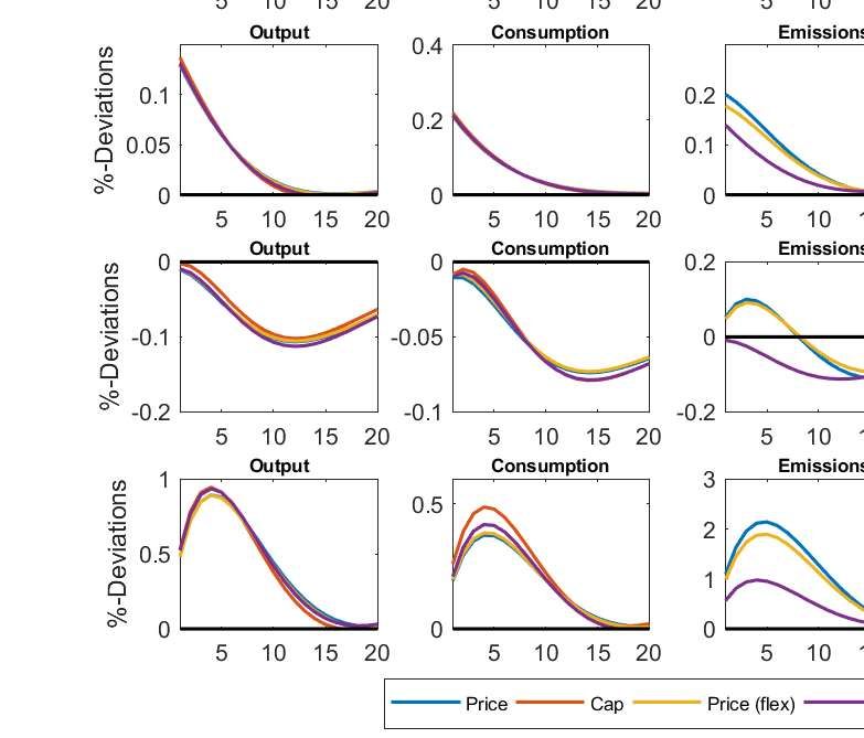
1 Introduction
The early work of Nordhaus (1977) has already stressed the fact that greenhouse gas (GHG) emissions
evolving as an external effect of economic activity affect atmospheric dynamics and spur global warming.
Today, most policymakers and academics reached a consensus that reducing GHG emissions in order to
alleviate global warming is a fundamental challenge the global community is facing at the moment. Due
to the potential consequences of temperature increases, such as floods, droughts and extreme weather
events, the goal is to limit the increase in global temperatures by meeting a certain carbon budget. This
ambition is reflected in the increasing number of national and supra-national initiatives that seek to reduce
emissions. As of today, the Carbon Pricing Dashboard of the World Bank reports over 50 different
initiatives either already implemented or scheduled for implementation. In general, these initiatives seek
to achieve emissions reductions through policy instruments that attach a price to emissions in order to
incentivize and promote a timely decarbonization of economic activity. Clearly, the transition towards a
carbon-neutral economy takes time, and the required structural adjustment is associated with costs. These
economic costs differ between policy instruments and are not necessarily uniformly distributed across
economic agents.
   Therefore, in order to implement climate policies efficiently and to avoid adverse distributional
consequences, it is important to understand how these policies affect economic activity and gauge their
distributional implications. In this context, Weitzman (1974) pointed out that economic uncertainty has
direct implications for overall welfare and the optimal choice of policy instruments. Based on this, a
strand of macroeconomic research developed to assess the implications of climate policies for short-run
macroeconomic dynamics under uncertainty. As documented by Doda (2014), GHG emissions fluctuate at
business cycle frequencies and tend to move procyclical with GDP. This implies that policies that reduce
emissions can also exert effects on short-run macroeconomic dynamics. Using a real business cycle
model, Heutel (2012) examines the effects of climate policies for macroeconomic dynamics and welfare.
He finds that emission policies should optimally behave procyclically. In a similar framework, Fischer
and Springborn (2011) compare taxes and quotas to intensity targets with regard to their implications for
macroeconomic volatility and welfare. They find that an intensity target exerts a comparatively small
effect on output, but implies larger volatility in labor markets relative to other instruments. Their results
suggest that from a welfare perspective, a tax is the preferable instrument. Dissou and Karnizova (2016)
compare a cap-and-trade system to a carbon tax within a multi-sectoral business cycle model and find that
a cap-and-trade system provides a more stable macroeconomic environment, but is deficient in terms of
welfare compared to a tax.
   Subsequent research on the macroeconomic implications of climate policy design has extended the
agenda in several directions. Annicchiarico and Dio (2015) examine climate policies within a New-
Keynesian business cycle model, taking nominal and real rigidities into account. Their results confirm
that taxes and intensity targets yield higher welfare but also imply a higher volatility in macroeconomic
aggregates compared to a cap-and-trade system. They also point out that the welfare effects of policy
instruments crucially depend on the degree of nominal frictions. In a similar framework, Annicchiarico
and Di Dio (2017) study the interactions between climate policy and monetary policy. They highlight
that these interactions have important implications for macroeconomic dynamics and the effectiveness
of climate policies. Another aspect studied by Annicchiarico and Diluiso (2019) within a two-country

                                                     1
New-Keynesian model are international spillover effects of climate policies. Their findings suggest that a
tax regime tends to amplify fluctuations while a cap-and-trade scheme alleviates spillover effects. They
highlight that the welfare effects of policy instruments depend on the type of shock and thus provide no
clear-cut ranking between the different policies.
   The present paper contributes to this strand of research in several ways. Primarily, we contribute
to the debate regarding the design of climate policies under uncertainty by taking distributional aspects
into account. This provides an important additional dimension for the assessment of different policy
instruments. While the analysis of Ohlendorf et al. (2020) highlights that the distributional effects of
climate policies have already been examined in various constellations, the short-run macroeconomic
perspective has largely been neglected. Building on a Two-Agent New-Keynesian (TANK) model, we
close this gap in the literature. As emphasized by Debortoli and Galı́ (2017), the presence of heterogeneous
households affects aggregate macroeconomic dynamics, and improves the empirical fit of these models.
Furthermore, we enrich the analysis by taking wage rigidites into account. This reflects the empirically
observed inertia and downward rigidity in wages and allows us to assess the distributional effects of
labor market frictions. Finally, we use this framework to assess uncertainties that directly evolve from
climate policies. These uncertainties fundamentally depend on our scientific knowledge and technological
possibilities. On the one hand, as argued by Fujimori et al. (2019), the estimates of the remaining carbon
budget, as published by the Intergovernmental Panel on Climate Change (IPCC), differ substantially across
studies and are subject to ongoing research. Advances in the understanding of atmospheric dynamics can
thus lead to revisions and updates of the carbon budget, which requires alignments of climate policies. On
the other hand, the technological abilities of the economy to reduce emissions vary over time. Conditional
on external factors such as weather or internal factors like the utilization of factor inputs, the emission
intensity of production can change. In order to comply with emissions reduction policies, these fluctuations
require economic adjustments.
   We calibrate the numerical model to match stylized aspects of the German economy and conduct
a comparison between price instruments, a cap-and-trade scheme and an intensity target policy. While
we find that those instruments do not alter the dynamics of macroeconomic aggregates qualitatively, we
observe quantitative differences in terms of volatility and aggregate welfare. In the present model, a cap-
and-trade system is associated with a larger volatility in output and consumption than other instruments.
The price instrument is preferable from a welfare perspective. Furthermore, for the baseline specification,
price instruments are found to exert neutral or even slightly progressive effects, while the intensity
target and the cap-and-trade system are found to be regressive. This finding results from the presence
of frictions and also depends on the utilization of the revenues from climate policy. When revenues
are redistributed via transfers, climate policy becomes moderately progressive. In terms of aggregate
welfare, the documented annual welfare costs associated with climate policy in Germany vary between
43 euros per capita under a price instrument with full redistribution, and 317 euros per capita under a
cap-and-trade scheme with full absorption of revenues. Furthermore, uncertainty associated with climate
policies alters macroeconomic dynamics and welfare and should not be neglected in the assessment
of policy instruments. A 10% change in the carbon budget requires substantial economic adjustments
associated with consumption and output losses. Through a staggered adjustment of policy instruments
these transitional costs can be alleviated. Nevertheless, the results of stochastic simulations highlight that
already the presence of carbon budget uncertainty is relevant for aggregate welfare.

                                                      2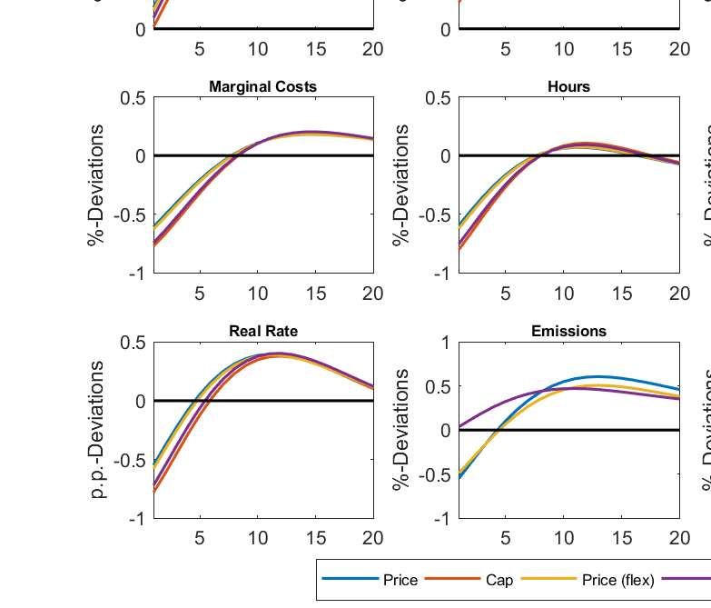
The remainder of this paper is structured as follows. The second section presents the theoretical model
and briefly discusses the set of policy instruments. The third section presents the calibration and the
numerical analysis of the model. Finally, the last section concludes the paper.

2 Model
2.1 Structure of the Model
In the following model, we focus on short-run macroeconomic dynamics and do not model the potential
adverse effects of climate change and the necessary long-run adjustments of production structures explicitly.
The model economy can then be interpreted in two ways. As emphasized by Annicchiarico and Dio (2015),
one view is that the economy has already accomplished the transition towards a carbon-neutral stationary
equilibrium. Alternatively, one can assume that the model economy moves along a deterministic balanced
decarbonization path. During the transition process, the economy is subject to aggregate uncertainty,
where different types of shocks induce fluctuations around the pathway and require economic adjustments.
    Formally, the model integrates carbon dioxide emissions that emerge as a by-product of production
as in Fischer and Springborn (2011) into a one-sector New-Keynesian model.1 As it is common in the
literature, we assume that firms operate under monopolistic competition and face nominal price setting
rigidities. Furthermore, we include real frictions in the form of convex investment adjustment costs, which
impedes adjustments of the stock of physical capital. Frictions on the labor market are introduced through
a union framework, where similar to the model of Erceg et al. (2000), nominal wage rigidities lead to wage
stickiness. In order to capture the effects of household heterogeneity and inequality, we follow Gali et al.
(2004) and distinguish between two types of households that differ in their ability to smooth consumption
via savings. The public sector, in terms of monetary and fiscal policy, follows the conventions in the
literature. Within this framework we assess the implications of different climate policy instruments in the
light of aggregate uncertainty.

2.2 Households
The economy is populated by a continuum of households I ∈ [0, 1]. In particular, we assume that two types
of households exist as in Gali et al. (2004).2 A fraction of households 1 − λ have access to capital markets
where they can accumulate physical capital kt and rent it to firms. These households will be referred to as
Ricardian households, indicated by the subscript R. The remaining fraction of households λ , who have no
access to capital markets and consequently own no assets, will be referred to as non-Ricardian households
with subscript N.

 1 As pointed out in Fischer and Heutel (2013), different ways to incorporate pollution into Dynamic Stochastic General
    Equilibrium (DSGE) models exist. For example Heutel (2012), uses a damage function approach, treating the stock of carbon
    dioxide as a state variable, comparable to the integration of pollution in most Integrated Assessment Models (IAM).
 2 The fact that a large fraction of households have no, or even negative net worth and thus behaves as rule-of-thumb consumers

    has already been stressed by Campbell and Mankiw (1989). Recent figures presented by Kuhn et al. (2018) show that in the
    United States between 1950 and 2016, the bottom 25% of the wealth distribution had almost zero net worth.

                                                              3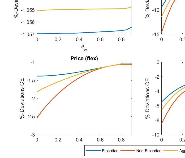
Ricardian Households

   The representative Ricardian household chooses consumption cR,t , investment xt and labor supply hR,t
in order to maximize expected life-time utility:

                                                   1−ρ                    1+χ
                                              "                                 #
                                    ∞             cR,t                hR,t
                                E0 ∑ dt β t                  − νt ψ                 , β ∈ (0, 1), χ > 0,        (1)
                                   t=0            1−ρ                 1+χ

where β denotes the discount factor of households, ψ denotes the disutility from labor, χ denotes the
inverse Frisch elasticity and ρ denotes the inverse of the intertemporal elasticity of substitution. The terms
dt and νt represent stochastic processes, i.e. a preference shock and a labor supply shock respectively.
The preference shock affects the time preferences of Ricardian households and evolves according to
dt = ρd dt−1 + εd,t , where ρd captures the persistence and εd,t the stochastic innovations of the process.
The labor supply shock evolves as νt = ρν νt−1 + εν,t , with persistence ρν and stochastic innovations in
labor disutility εν,t . The optimization of Ricardian households is subject to a flow budget constraint. In
real terms, the constraint reads:

                                                                      bt−1
                            cR,t + xt + bt = Wt hR,t + Rt−1                + Fu,t + FF,t + Rk,t kt − Tt ,       (2)
                                                                       Πt

here Wt denotes the real remuneration of labor supplied to a union. The real return of capital is denoted by
                                          pt
Rk,t , inflation is denoted by Πt =      pt−1 ,   bt denotes the stock of risk-free one period government bonds, Rt
denotes the nominal interest rate and Tt denotes a lump-sum tax levied by the government. Since firms are
owned by Ricardian households, they receive firm profits FF,t and a share of union profits Fu,t .
   In order to capture the fact that capital cannot be adjusted instantaneously at business cycle frequencies,
convex investment adjustment costs, similar to Christiano et al. (2005), are introduced as follows:
                                          "                          2 #
                                            κ                 xt
                                 kt+1 = 1 −                         −1     zt xt + (1 − δ )kt        .          (3)
                                            2                xt−1

Here, κ captures the degree of adjustment costs and δ denotes the depreciation rate. With this formulation,
the costs of investment increase in the growth rate of investment. Thus, large increases in investment
in a single period are particularly expensive, which implies that households will spread investment over
several periods. Therefore, adjustments of the stock of physical capital require time. The term zt denotes
investment efficiency, i.e. the efficiency to transform investments into physical capital. We assume that
investment efficiency is subject to stochastic fluctuations, which are given by zt = ρz zt−1 + εz,t , where ρz
captures the persistence and εz,t the stochastic innovations of the process. The inclusion of investment
shocks is motivated by the findings of Khan et al. (2019), who show that investment shocks appear to be
an important determinant for the fluctuations in emissions.
   The solution of the household problem yields the following first-order conditions for consumption,
labor supply, bond holdings, capital and investment:

              −ρ
  λR,t = dt cR,t                                                                                                (4)
           νt ψhR,t Wt −1
                χ
  λR,t =                                                                                                        (5)

                                                                      4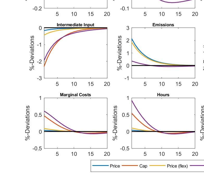
−1
      λR,t = β Rt Et λR,t+1 Πt+1                                                                                                 (6)
                                   2                   !
                                                                                            xt+1 2

                       κ     xt           xt        xt           λR,t+1          xt+1
        1 = qt 1 −               −1 −κ        −1          + β Et        qt+1 κ        −1                                         (7)
                       2 xt+1            xt−1      xt−1           λR,t            xt         xt
                     λR,t+1 zt
         qt = β Et              ((1 − δ )qt+1 + zt+1 RK,t+1 ) .                                                                  (8)
                      λR,t zt+1

Here λR,t denotes the marginal utility of an additional unit of consumption and qt denotes Tobins q, which
captures the value of installed capital relative to new capital.3 Therefore, the relative price of installed
capital can deviate from the price of newly built capital.

Non-Ricardian Households

        Non-Ricardian households are not able to smooth consumption through saving and thus seek to
optimize their utility period-by-period. In the following, we assume that the utility function is additive-
                                                           1−ρ           1+χ
                                                          cN,t           h
separable and has the functional form: uN =               1−ρ
                                                                          N,t
                                                                 − νt ψ (1+χ) .4 In the absence of access to capital markets,
non-Ricardian households face a constraint, which restricts their consumption cN,t to their current income,
i.e. cN,t = Wt hN,t − Tt + Fu,t . The labor supply of non-Ricardian households hN,t is given by:

                                                                         −ρ
                                                         νt ψhN,t = cN,t Wt
                                                                 χ
                                                                                                                                 (9)

which in this case is not constant and depends on the real labor remuneration and the marginal utility
from consumption.5 Aggregate household consumption ct and aggregate labor supply ht correspond to
the weighted averages of the individual variables and are defined as:

                                                    ct ≡ λ cN,t + (1 − λ )cR,t
                                                    ht ≡ λ hN,t + (1 − λ )hR,t .

Union Wage Setting

        In order to introduce inertia in wage adjustments, we follow the approach of Sims and Wu (2019)
and assume that households supply differentiated labor inputs to a continuum of unions u ∈ [0, 1].6
Unions remunerate households and sell labor inputs hu,t to a competitive labor packer at the price
wu,t . The labor packer uses a constant elasticity of substitution (CES) aggregator, given by hd,t =
R 1 (ηw −1)/1
(   0   hu,t      du)ηw /(ηw −1) , to transform differentiated union labor into final labor input for the production

    3 More   formally, Tobins q represents the marginal utility of having an additional future unit of installed capital kt+1 over the
       marginal utility of having an additional unit of consumption.
    4 While labor supply of non-Ricardian households is subject to the same shock ν as the labor supply of Ricardian households,
                                                                                      t
       they do not face preference shocks.
    5 If the utility function is non-separable in consumption and leisure, the labor supply of non-Ricardian households remains

       constant. As shown by Gali et al. (2004), this also implies that consumption of non-Ricardian households will always be
       proportional to their wage income. This would imply that variations in the income of non-Ricardian households are solely
       driven by fluctuations in wages. Under the present assumptions, variations in working hours constitute an additional source
       of variation for the income of non-Ricardian households.
    6 As in Galı́ et al. (2007), we assume that the distribution of differentiated labor types is identical across both groups of

       households.

                                                                     5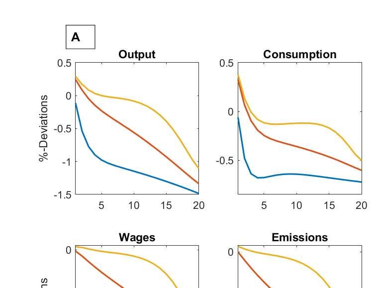
sector. Profit maximization of the labor packer yields demand curves for each type of union labor relative
to aggregate labor demand of the production sector hd,t :
                                                                      −ηw
                                                                wu,t
                                                   hu,t =                     hd,t                                          (10)
                                                                wt

where ηw > 1 denotes the elasticity of substitution between differentiated labor inputs and wt denotes the
aggregate real wage, which evolves according to wt1−ηw =
                                                                          R 1 1−ηw
                                                                              0   wu,t   du.
    Each union transforms the labor supply of households one-for-one and seeks to set its wage in order
to maximize the income of union members by maximizing the transfer Fu,t which union members receive.
However, wage setting of unions is subject to a nominal rigidity ala Calvo (1983). Every period unions
can adjust the wage with probability 1 − θw . This implies that a wage set in period t can persist for several
periods k. Unions take this possibility into account and apply the stochastic discount factor of Ricardian
                           λi,t+k
households Λt,t+k = β       λi,t    in order to maximize the expected present discounted value of their members’
labor   income.7   Under these assumptions, the optimal reset wage wt∗ is common across unions and reads:

                                                           Et ∑∞      k
                                              ηw                k=0 θw Λt,t+k
                                     wt∗ =                              ηw −1          .                                    (11)
                                             ηw − 1 Et ∑∞    k
                                                        k=0 θw Λt,t+k wt+k pt+k hd,t+k

    It can be inferred, that in absence of wage adjustment rigidities, unions will set wages as a markup
 ηw
ηw −1   above the level of competitive wages. In addition, the presence of the nominal rigidity induces
inertia in wages and alters labor market dynamics. This is also reflected in the dynamic evolution of the
aggregate real wage, which can be derived as a weighted average of currently adjusted and past wages:

                                      wt1−ηw = (1 − θw )wt∗1−ηw + θw Πtηw −1 wt−1
                                                                              1−ηw
                                                                                   .                                        (12)

2.3 Firms
The production sector of the economy can be divided into two layers. Final goods producers operate under
perfect competition and aggregate intermediate goods into final output yt . The intermediate goods y j,t are
produced by a continuum of intermediate firms j ∈ [0, 1] under monopolistic competition. Intermediate
firms face nominal price rigidities as in Calvo (1983). Furthermore, as in Fischer and Springborn (2011),
in order to produce output, intermediate firms rely on a polluting intermediate input factor m j,t . For
simplicity, we assume that they buy the polluting intermediate factor in exchange for final goods at the
price pm,t .8
                                                                                           R 1 (ε−1)/ε
    Final goods producers use a CES aggregator of the form yt = (                              0   y j,t   d j)ε/(ε−1) to combine
intermediate goods into final goods. Here ε > 1 denotes the elasticity of substitution between different
varieties of intermediate goods. Profit maximization of final goods producers yields the usual downward
                                                            p j,t −ε
sloping demand for intermediate goods y j,t = (              pt ) yt .    The demand for the intermediate good j is a
decreasing function of the individual price of the intermediate good p j,t relative to the overall price level
 7 This  assumption seems warranted since the parameters of the utility function are similar across both types of households.
    Alternatively, as in Colciago (2011), one could assume that unions maximize the weighted sum of household utility across
    Ricardian and non-Ricardian households.
 8 As is common in the literature on energy and business cycles, we assume that p
                                                                                 m,t is exogenously given, cf. Kim and Loungani
    (1992). Note that we also assess the implications of exogenous fluctuations in pm,t and the resulting dynamics are largely
    comparable to those of uncertainty about emissions prices and are available upon request from the author.

                                                                 6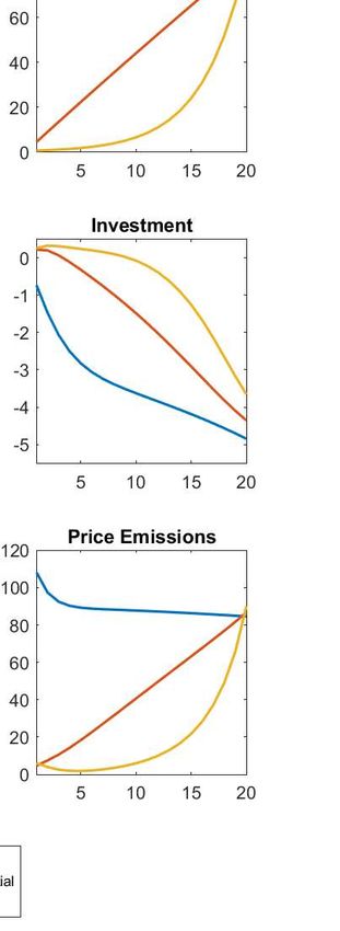
of intermediate goods pt . Using the demand for individual goods, the price level of the economy, defined
                                                                              R 1 1−ε      1/(1−ε) .
as the sum over intermediate prices times quantities, is pt = (                0 p j,t d j)
    Regarding the production technology, we adopt the formulation of Bosetti and Maffezzoli (2014).
Intermediate firms produce according to the following constant returns to scale technology:

                          y j,t = At (kαj,t h1−α     1−γ    γ
                                             d, j,t )    m j,t ,       0 < α < 1,             0 < γ < 1,       (13)

where At represents total factor productivity (TFP) which evolves as At = ρa At−1 + εa,t . Here ρa denotes
the autocorrelation of the AR(1) process and εa,t denotes the innovations in productivity that are assumed
to be i.i.d. normally distributed. The output elasticity of the polluting intermediate input is denoted
by γ and α denotes the output elasticity of physical capital. As explained, we assume that emissions
e j,t are proportional to the utilization of the polluting intermediate input, i.e. e j,t = φe,t m j,t . The degree
of proportionality thus depends on φe,t . Now, in order to introduce uncertainty regarding the emission
intensity of production, we assume that φe,t evolves as:

                                        φe,t = (1 − ρφe )φ¯e + ρφe φe,t−1 + εφe ,t            .                (14)

Here φ¯e denotes the steady state emission intensity, which we normalize to unity as in Fischer and Spring-
born (2011), ρφe denotes the persistence of fluctuations in emission intensity and εφe ,t are independent
innovations in emission intensity. This formulation can be regarded as a reduced-form approach that
reflects a general uncertainty about technological abilities to absorb or abate emissions in production.
    Intermediate firms take factor prices as given, so that in the absence of emission reduction policies,
their static cost minimization problem yields the following optimality conditions for factor inputs:

                                 Rk,t = λ j,t (1 − γ)αAt (kαj,t h1−α     1−γ
                                                                             m j,t k−1
                                                                                   γ
                                                                 d, j,t )           j,t                        (15)
                                  wt = λ j,t (1 − γ)(1 − α)At (kαj,t h1−α     1−γ
                                                                                  m j,t h−1
                                                                                          γ
                                                                      d, j,t )           d, j,t                (16)
                                pm,t = λ j,t γAt (kαj,t h1−α     1−γ    γ−1
                                                         d, j,t )    m j,t     .                               (17)

Here, the Lagrange multiplier λ j,t = mc j,t can be interpreted as marginal costs of the firm, i.e. the cost
of producing an additional unit of output. From (17) we can infer that at the optimum, firms choose
the amount of the polluting intermediate input, such that marginal revenues equate marginal costs. This
implies that regulatory measures that increase the cost of employing intermediate inputs, such as permit
requirements or a tax, will distort the choice of input factors and incentivize firms to reduce emissions.
Furthermore, conditions (15) - (17) imply that all firms will choose the same capital-labor and intermediate
inputs-labor ratios so that marginal costs are common to all firms, i.e. mc j,t = mct , where:

                                            1−γ                  α(1−γ)  γ (1−α)(1−γ) α(1−γ) γ
                                                                            1 wt          Rk,t   pm,t

                              1                       (1 − α)
            mct =                                                                                          .   (18)
                        (1 − α)(1 − γ)                   α                  γ            At

    Intermediate goods producers use their market power and choose the price of intermediate goods p j,t
that maximizes discounted real profits. To this end, they apply the stochastic discount factor of Ricardian
                                         λR,t+i
households defined as Λt,t+i = β          λR,t .   Price stickiness is introduced according to Calvo (1983), every
period only a fraction (1 − θ p ) of firms can adjust their prices. The firms that cannot adjust their prices

                                                                   7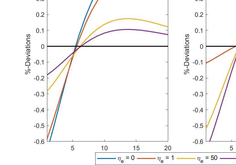
remain at their previously chosen prices. The solution to this dynamic price-setting problem implies that
all firms that can reset prices will choose the same optimal reset price pt∗ , given by:

                                                 ε Et ∑i=0 θ pi Λt,t+i pt+i
                                                        ∞               ε y mc
                                                                            t+i  t+i
                              pt∗ = p j,t =                                                   .                         (19)
                                              (ε − 1) Et ∑∞     θ iΛ     p ε−1
                                                          i=0 p t,t+i t+i t+i  y

With θ p = 0, all firms can freely adjust their prices and the price of intermediate goods will be a markup
  ε
(ε−1)   > 1 over marginal costs. With θ p > 0, the evolution of the aggregate price level is given by
pt = [(1 − θ p )pt∗1−ε + θ p pt−1
                              1−ε 1/(1−ε)
                                  ]       , which implies that the current aggregate price level corresponds
to the weighted average of recently adjusted and previous prices. For later reference, we rewrite this in
                                                                                              pt∗
terms of inflation as 1 = (1 − θ p )Πt∗1−ε + θ p Πtε−1 , where Πt =       pt
                                                                         pt−1   and Πt∗ =     pt .   Finally, using the Calvo
assumption, the price dispersion in equilibrium        vtp   can be written as   vtp                                p
                                                                                       = (1 − θ p )Πt∗−ε + θ p Πtε vt−1 . The
profits of firms FF,t are distributed lump-sum to Ricardian households.

2.4 Environmental Policies
In the present model, environmental regulation is conducted through an independent institution such
that the revenues of the carbon reduction scheme in place, denoted as Te,t , are not necessarily part of
the government budget. In modeling the environmental regulator, we follow the general principals as
laid out in the proposal of Delpla and Gollier (2019). This entails that the policies under consideration
follow the polluter pays principle, i.e. the costs of emissions have to be borne by the entity that emits
carbon dioxide. In the model, emissions result from the utilization of a polluting intermediate input by
intermediate goods producers. Hence, climate policies directly affect the production side of the economy
and alter the optimization problem of intermediate firms.
    In the following, we consider four different policy instruments. A constant price instrument (compara-
ble to a tax), a flexible price instrument where the price of emissions adjusts dynamically, a cap-and-trade
system where the price of permits is formed in competitive permit markets, and an intensity target. This
set of instruments spans the space between fully flexible emissions at a constant price under the price
scenario and fixed emissions at fully flexible prices under the cap-and-trade scenario. In contrast, the
flexible price and the intensity target allow for fluctuations of both prices and quantities. The main
difference between the later instruments is that the flexible price scheme dampens the procyclical reaction
of emissions, whereas the intensity target allows firms to adjust emissions procyclically. As documented
by Heutel (2012), this distinction is important. According to his analysis, policies that allow for procyclical
emissions adjustments in response to fluctuations tend to be preferable from a welfare perspective.
    To illustrate the different policy instruments, we use the fact that from the perspective of interme-
diate goods producers, the unit costs associated with intermediate inputs p̂m,t can be broken into two
components. Formally, p̂m,t = pm,t + φe,t pe,t , where pe,t denotes the price of emissions under the different
policy instruments g(·), such that pe (g(·)). Thus, emissions policies alter the optimization problem of
intermediate goods producers by increasing the costs of intermediate inputs. Taking this into account,
firms’ marginal costs under emission policies are given by:

                                           1−γ              α(1−γ)  γ (1−α)(1−γ) α(1−γ) γ
                                                                       1 wt          Rk,t   p̂m,t

                                1                   (1 − α)
              mct =                                                                               .                     (20)
                          (1 − α)(1 − γ)               α               γ            At

                                                              8
We assume that under the price instrument, the unit price of emissions is fixed at the exogenous level
pe = µ. In case of the cap-and-trade scenario, we assume that firms face a constantly binding emissions
constraint et = ē and that one unit of emissions requires firms to provide one unit of permits. The number
of permits issued by the regulator is kept constant over time. Under the flexible price scheme, the price
of emissions takes the form of a reaction function pe,t = µ + ηe (et − ē), and depends on the level of
emissions relative to steady state emissions. The parameter ηe captures the intensity in which the emission
price reacts to deviations of emissions from the target. Finally, the intensity target requires et = ξ yt , i.e.
the emissions to output ratio is fixed at the exogenous value ξ . Note that we assume that intermediate
goods producers trade permits in a perfectly competitive market. Thus, in the case of quantity instruments,
the price of emissions corresponds to ωt , i.e. the shadow value of an additional permit resulting from the
optimization of firms under the emission constraint.             9   Table 1 summarizes the different instruments and
the corresponding price of the intermediate input.

                Instrument            Functional form                  Price of intermediate inputs
                Price                 g(et ) = µ                       p̂m,t = pm,t + φe,t µ
                Flex Price            g(et ) = µ + ηe (et − ē)        p̂m,t = pm,t + φe,t (µ + ηe (et − ē))
                Cap-and-Trade         g(et ) = et ≤ ē                 p̂m,t = pm,t + φe,t ωt
                Intensity Target      g(yt , et ) = et ≤ ξ yt          p̂m,t = pm,t + φe,t ωt

                      Table 1: Climate policy instruments and intermediate input prices.

    As can be inferred, all policy instruments attach a price to emissions that translates into a price increase
of intermediate inputs. This induces two types of adjustments on the supply side of the economy. First,
in response to an increase in p̂m,t , firms adjust the proportion of input factors and reduce the amount of
the polluting intermediate goods used in production. To see this, combine (16) and (17) under an active
climate policy, to obtain the optimal factor input ratio of the polluting intermediate good vis-a-vis labor:

                                              mt           γ         wt
                                                   =                      .
                                              hd,t   (1 − α)(1 − γ) p̂m,t

Apparently, an exogenous increase in p̂m,t requires ceteris paribus a decline in mt /hd,t .10 Given the under-
lying production structure, firms react to the change in relative factor prices by substituting intermediate
inputs through additional capital and labor. This substitution effect has implications for the deterministic
steady state of the economy and also determines the short-run dynamics in response to shocks. In general,
the deterministic long-run adjustments of factor inputs depend on the relative productivity of input factors.
In the present model, at the same emissions reduction goal, all policy instruments lead to identical long-run
adjustments, i.e. the same deterministic steady state. However, in the short-run with frictional adjustment,
by design, all four instruments differ in terms of price and emissions dynamics.
    Furthermore, as depicted in (19), the dynamic price setting decision of firms is based on current and
expected future production costs. Hence, an increase in the user costs of polluting intermediate goods will
lead to price adjustments on the firm level, followed by a corresponding increase in the aggregate price

 9 Formally, at the optimum, firms equate the marginal gains from using an additional unit of emissions to its costs, thus ωt
    represents the Lagrange multiplier associated with the emissions constraint.
10 This follows from: ∂ (mt /hd,t ) < 0.
                         ∂ p̂
                          m,t

                                                             9
level. On the one hand, as implied by (6), this affects the consumption decisions of Ricardian households.
On the other hand, the inflationary impulse leads to interactions between climate, monetary and fiscal
policies. To the extent that the effect on the emission price differs between the instruments, this will alter
macroeconomic dynamics in response to shocks.
Finally, as laid out in the introduction, the actual size of the global emissions budget is subject to
uncertainty. To capture this, we assume that environmental policies are fully committed to the desired
emissions reduction goal and therefore adjust the policy instruments accordingly. This implies that an
unexpected adjustment in available emissions translates directly into adjustments of the price of emissions
or the number of emissions permits issued under price or quantity regulations, respectively. Formally, we
will introduce this uncertainty about the emission budget as follows:
ēt = (1 − ρe )ē + ρe ēt−1 + εe,t , (21)
where ρe denotes the persistence of changes in the carbon budget and εe,t denotes the stochastic innovations
in the emission cap.11
2.5 Public Sector and Market Clearing
Central Bank
The short-term gross nominal interest rate Rt is under the control of the central bank, which has the
objective to maintain price stability and reacts to deviations of inflation from inflation target Π̄. Monetary
policy is conducted according to the monetary policy rule:
γR γΠ 1−γR
Rt Rt−1 Πt
= exp(εR,t ) . (22)
R̄ R̄ Π̄
Here, γΠ denotes the coefficient that captures the reaction of the central bank to deviations of inflation
from the target and γR captures the persistence in nominal interest rates and ensures empirically plausible
smooth adjustments in nominal rates. The steady state nominal interest rate is denoted by R̄, and εR,t
denotes stochastic innovations in the nominal rate.
Government
Since the main focus of the present analysis is on environmental policies, the government sector is
kept rather simple. In particular, we abstract from distortionary taxation apart from climate policies. In
real terms, the government flow budget constraint is given by:
gt + Rt−1 bt−1 /Πt = bt + Tt + TE,t (23)
i.e. real government expenditures gt are financed via issuing risk-free bonds bt through lump-sum taxes Tt
levied upon households and through the revenues of the emission reduction scheme in place TE,t = pe,t et .
11 Incase of a price instrument, innovations in the carbon budget induce adjustments of the carbon price. Formally pe,t =
(1 − ρe )µ + ρe pe,t−1 + εe,t , where the mapping between µ and ē can be used to generate equivalent fluctuations in prices.
10To ensure the long-run sustainability of government debt, the governments follows the fiscal rule:
Tt = T̄ + φT (bt − b̄) (24)
where T̄ denotes steady state taxes and φT captures the intensity of adjustments in taxes in response to
deviations of the stock of government debt from an exogenously defined target b̄. Government expenditures
are stochastic and follow the AR(1) process gt = (1 − ρg )ḡ + ρg gt−1 + εg,t . Here, ḡ denotes an exogenous
target of government consumption and ρg captures the persistence of i.i.d. innovations in government
consumption denoted by εg,t .
Aggregation and Market Clearing
In equilibrium factor and goods markets clear. Labor market clearing requires that the labor supply of
unions equates the labor demand of the labor packer, which under perfect competition corresponds to labor
R1
demand of intermediate good producers. Aggregate labor supply is given by 0 hu,t du = ht taking the
demand function for differentiated labor (10) into account, we have ht = hd,t vtw , where vtw denotes wage
R w
dispersion, defined as vtw = 01 ( wu,t )−ηw du. Given the wage adjustment frictions, the dynamic evolution
t
of wage dispersion is given by:
−ηw
wt∗
ηw
wt
vtw = (1 − θw ) + θw Πtηw w
vt−1 . (25)
wt wt−1
R1 R1
Market clearing for capital and intermediate inputs implies: kt = 0 k j,t d j and mt = 0 m j,t d j. Taking the
R1 R 1 p j,t −ε p
demand for intermediate goods into account, integration yields 0 y j,t d j = 0 ( pt ) yt d j = yt vt , where
vtp evolves dynamically as defined above. Aggregate final output can thus be written as:
yt = At (ktα h1−α 1−γ
mt /vtp .
γ
d,t ) (26)
Since vtp > 1, if θ p > 0, price dispersion reflects the inefficiency of aggregate output associated with price
rigidity. The resource constraint of the economy requires:
yt = xt + ct + gt + p̂m,t mt , (27)
where p̂m,t mt includes the revenues of the environmental policy regime whenever they are not part of the
government budget. A full summary of the equilibrium conditions for the baseline scenario, as well as
details regarding the solution procedure, are provided in 5.2.
3 Quantitative Analysis
This section presents the quantitative evaluation of the theoretical model. Since no solution to the full
non-linear model exists, the model is solved numerically using a second-order Taylor approximation
around the deterministic steady state of the model. The first part of this section compares the four policy
instruments, and assesses the resulting implications for macroeconomic dynamics in response to different
11sources of business cycle fluctuations. This exercise includes a comparison of macroeconomic stability
and welfare across instruments. Subsequently, we evaluate the distributive implications of the policy
instruments and examine the role of uncertainty and frictions in this context. In the second part of the
analysis we focus on uncertainty regarding the carbon budget. Here, we incorporate carbon budget
shocks into the model. We begin with an examination of the macroeconomic dynamics in response to an
unexpected change in the carbon budget, which leads to adjustments of climate policy instruments and
compare the implications of a price instrument to those of a cap-and-trade scheme. Afterwards, we use
the stochastic model with fluctuations in the emission cap and the emission price to examine the general
role of uncertainties associated with the carbon budget.
3.1 Calibration
The numerical simulations require defining specific parameter values. As is common in the literature,
the model is calibrated to capture some empirically observed moments of the economy. In particular,
we try to match the dynamics of output and consumption of the German economy. To this end we
specify the parameters of the production sector based on empirical data to match the average ratios of
private consumption to GDP and private investment to GDP. The share of polluting intermediate inputs
in production is set to match the share of energy in production. Parameters which reflect monetary and
fiscal policy are set to match the average inflation rate, the ratio of government consumption to GDP
and the debt to GDP target. Regarding the structural parameters of the model, which capture household
preferences and frictions, we largely follow the existing literature on German business cycles. Table 2
summarizes the parameters used in the baseline specification.
The parameters that capture household preferences correspond to the values used by Hristov (2016).
The subjective discount factor of households is set to 0.998, the inverse of the intertemporal elasticity of
substitution is set to ρ = 2 and the inverse of the Frisch elasticity of labor supply χ is set to 1.5. These
values are broadly in line with values used in most studies of the German economy. Based on the results
reported by Grabka and Halbmeier (2019), the share of non-Ricardian households λ is set to 0.28. 12 The
wage-setting frequency of unions θw is taken from Gadatsch et al. (2016) and set to 0.83. The elasticity of
substitution between labor types is set to ηw = 4. This implies a wage markup in the deterministic steady
state of 1.33. Finally, the labor disutility parameter ψ is set in order to reach an average working time of
ht = 0.33 in the deterministic steady state.
We set the capital share to α = 0.3, which corresponds to the average capital share in Germany
between 1990 and 2015 as reported by the Federal Statistical Office (Destatis). Fischer and Springborn
(2011) calibrate the production elasticity of polluting intermediate inputs γ to match the average energy
expenditures relative to GDP in the United States. For Germany, we set γ = 0.1, which corresponds to the
average total energy supply relative to GDP as reported by the International Energy Agency (IEA) for the
period from 1990 – 2015. The quarterly depreciation rate of physical capital δ is set to 0.025. In line with
the estimation results of Drygalla et al. (2020), we set the investment adjustment cost parameter κ to 3.9.
According to the estimation results of Jondeau and Sahuc (2008) for the Germany economy, we set the
12 Awell documented phenomenon is the occurrence of indeterminacy of equilibrium, conditional on the share of non-Ricardian
households and the degree of price adjustment frictions. In the given model, this issue arises for a share of non-Ricardian
households of 70% and at values of θ p > 0.7. The corresponding plot illustrating parameter combinations associated with
indeterminacy of the model is provided in appendix 5.3.
12Calvo parameter to θ p = 0.86 and the elasticity of substitution between intermediate goods ε to 6, which
corresponds to a markup of 1.2.13
Regarding the choice of the parameters that capture monetary and fiscal policy, we again consider the
estimation results of Drygalla et al. (2020). The stance on inflation γΠ is set to 1.47 and the degree of
interest rate smoothing γR is set to 0.91. The target rate of inflation is set to 1%.14 The parameter φT that
captures the strength of the reaction of lump-sum taxes to deviations of government debt from target is set
to 0.38. As explained, the steady state levels of government debt b̄ and consumption ḡ are set to match a
debt-to-GDP ratio of 0.6 and a government consumption to GDP ratio of 0.19.15
In the first exercise, we test the implications of climate policies for short-run macroeconomic dynamics.
Since the studies on German business cycles cited above differ in terms of models and sample periods, we
cannot adopt all their estimates of the shock processes directly. Therefore, we use the reported results
and set the autocorrelations and standard deviations of shock processes within the reported range.16 The
uncertainty of emission intensity, formally described by (14), is specified in line with the properties of
quarterly emission intensity data for Germany. The corresponding time series ranging from 1991Q3 to
2012Q4, is constructed using data on carbon dioxide emissions from Crippa et al. (2020) and data on
real GDP obtained from Destatis. The cyclical component of emission intensity is found to be relatively
persistent with a statistically significant autocorrelation of ρφe = 0.78 and σφe = 0.023.17 Overall, the
employed parameter values are comparable to the literature and are summarized at the bottom of table 2.
In the second exercise, in order to assess the role of carbon budget uncertainty, we extended the
baseline model by equation (21). Uncertainty about the remaining carbon budget evolves for several
reasons. First of all, carbon budgets differ with respect to the specific climate goal. Clearly, keeping
global warming below 2°C is associated with a larger remaining carbon budget compared to keeping
the temperature increase below 1.5°C. But even for a specific climate goal, carbon budgets differ due to
scientific uncertainty about atmospheric dynamics. Furthermore, some decarbonization pathways allow
for overshooting, which keeps the carbon budget more flexible. To specify the uncertainty in the carbon
budget, we restrict the space of carbon budgets to the 1.5°C scenarios as reported by IPCC (2018). Then
we proceed in two ways. First, we extract all scenarios from Huppmann et al. (2019) and follow Fujimori
et al. (2019), who compute the remaining cumulative CO2 emissions for each study. Based on the reported
carbon budgets, we obtain a relative standard deviation in the estimates of the remaining carbon budget of
σe = 0.060. In addition, we also compute the standard deviation in the reported budgets, including studies
which allow for low-overshooting. Based on 51 studies, we obtain a relative standard deviation in the
carbon budgets of σe = 0.126. However, these studies can differ with respect to the assumptions regarding
emission absorption technologies and therefore partially capture technological uncertainty as well. A
second approach is based on the information provided by Rogelj (2018), where based on the transient
climate response (TCR) to cumulative emissions of carbon within the 1.5°C scenario we obtain a relative
13 As documented by Annicchiarico and Dio (2015), the degree of nominal frictions has strong implications for the relative
performance of climate policy instruments. We therefore assess this issue explicitly in a following analysis.
14 These parameter values fulfill the Taylor principle and ensure that the stationary equilibrium is uniquely determined.
15 The debt-to-GDP ratio is chosen in accordance with the Maastricht criteria and the ratio of government consumption
corresponds roughly to the empirically observed share of government consumption over GDP in Germany between 1991 –
2016, as reported by Destatis.
16 In addition, we also take the estimation results of Pytlarczyk (2005) and Gadatsch et al. (2015) into account.
17 As is common in the literature, the cyclical component is obtained applying the HP-Filter with λ = 1600. More details on the
data used in the calibration and additional information are presented in 5.1.
13Parameter Value Description
Households:
β 0.998 Subjective discount factor
χ 1.5 Inverse Frisch elasticity
ρ 2 Inverse elasticity of intertemporal substitution
ψ 45 Labor disutility
λ 0.28 Share of non-Ricardian households
θw 0.83 Wage adjustment frictions (unions)
ηw 4 Elasticity of substitution labor types
Firms:
δ 0.025 Depreciation rate
γ 0.1 Output elasticity polluting goods
α 0.30 Output elasticity capital
κ 3.9 Investment adjustment costs
θp 0.86 Price stickiness
ε 6 Elasticity of substitution intermediate goods
Polices:
γΠ 1.47 Interest rate rule inflation coefficient
γR 0.91 Interest rate rule smoothing coefficient
Π̄ 1.01 Target inflation
φT 0.38 Reaction of taxation
b
y 0.6 Debt-GDP-ratio
g
y 0.19 Government consumption to GDP ratio
Stochastic processes:
ρa 0.95 Persistence TFP shock
ρg 0.86 Persistence government spending shock
ρd 0.82 Persistence preference shock
ρν 0.88 Persistence labor supply shock
ρz 0.77 Persistence investment shock
ρφ 0.78 Persistence emission intensity shock
σa 0.0049 S.D. TFP shock
σR 0.0004 S.D. Monetary shock
σg 0.0039 S.D. Government spending shock
σν 0.0118 S.D. Labor supply shock
σd 0.0044 S.D. Preference shock
σz 0.0183 S.D. Investment shock
σφ 0.023 S.D. Emission intensity shock
Table 2: Calibrated Parameters – Baseline Scenario
standard deviation of σe = 0.167.18 Thus we see that overall variations in carbon budget estimates fall
into a broad range between 0.060 < σe < 0.167.
3.2 Business Cycle Shocks – Volatility and Welfare
First, to compare the implications of the present model formulation to previous studies and to understand
the role of heterogeneity in income and wealth in light of emissions reduction policies, we examine the
response of the economy to six frequently examined business cycle shocks. In particular, we focus on
supply shocks, which are modeled as fluctuations in total factor productivity, demand shocks, which take
the form of preference shocks, shocks to the nominal interest rate, i.e. monetary policy shocks, shocks to
18 We consider all scenarios within the 67% percentile and compute emission budgets from 2011 onward.
14investment efficiency, shocks to government consumption and labor supply shocks. This wide range of
shocks captures several relevant drivers of business cycles. In addition to the common sources of business
cycle fluctuations, we allow for stochastic innovations in emission intensity, based on the estimated shock
processes for the German economy. In the absence of climate policy, emission intensity shocks only affect
emissions but do not alter aggregate dynamics. However, under an active climate policy, fluctuations in
emission intensity affect the optimal utilization of input factors and can exert effects on macroeconomic
aggregates.
In the baseline scenario, we assess the effects of a 10% reduction in emissions for the deterministic
steady state of the model relative to a no-policy scenario. This reflects a situation in which climate policies
require emissions adjustments on the firm level. The policy parameters µ, ē and ξ , which capture the
price of emissions, the emissions cap and the intensity target, respectively, are calibrated to yield the
same level of steady state emissions. The parameter ηe that captures the reaction of emission prices to
deviations from the target is set to 5.19 Overall, the reduction target is set to ensure a constantly binding
emissions constraint when considering quantity instruments. The revenues generated through emissions
policies are completely absorbed.20 Table 3 provides a comparison of key macroeconomic variables and
welfare between the no-policy case vis-a-vis the 10% reduction scenario in the deterministic steady state.
Scenario yt kt ht et ct xt Welfare
No-Policy 0.534 4.462 0.333 0.044 0.274 0.112
(% change) 0 0 0 0 0 0
Policy 0.529 4.414 0.336 0.040 0.271 0.110
(% change) -1.1% -1.1% 0.4% -10.0% -1.1% -1.1% -1.05%
Table 3: Comparison of macroeconomic aggregates in the deterministic steady state under climate policy
and percentage changes relative to the no-policy scenario. Welfare effects are expressed as
consumption equivalent variations relative to the no-policy scenario.
As can be inferred, compared to the no-policy case, a 10% emissions reduction leads to a decline in
output of roughly 1.1%. The relative decline in the physical capital stock, aggregate consumption and
investment are of the same magnitude. Since firms substitute the polluting intermediate good partially by
employing additional labor, we see a small increase in aggregate working hours of about 0.4%. In terms
of consumption equivalent variations, aggregate welfare declines by about 1.05% relative to the no-policy
scenario. Quantitatively, the results are by and large comparable to the results presented by Annicchiarico
and Dio (2015) and Fischer and Springborn (2011), and the implied steady state ratios for the no-policy
scenario are close to empirically observed statistics for Germany.21
19 Appendix 5.4 illustrates the effects of the choice of ηe on model dynamics for a TFP shock. In general, a larger reaction
parameter tends to dampen the observed dynamics.
20 This assumption corresponds to a scenario in which the revenues of climate policies are treated as an increase in the import
price of natural resources and therefore flow out of the small open economy. While this assumption is clearly arbitrary, it
provides an unbiased reference point to compare policy instruments in the absence of changes to fiscal policies.
21 While the model matches the target value for government consumption over GDP, the implied ratio of private consumption to
GDP of ct /yt ≈ 0.51 and the ratio of private investment to GDP of xt /yt ≈ 0.21 in the no-policy scenario are also comparable
to the values observed for the German economy between 1991 and 2015.
15Impulse Responses
We begin with a graphical examination of the model dynamics under the four different policy regimes
in response to aggregate shocks. All results are based on the baseline parameter values and refer to a
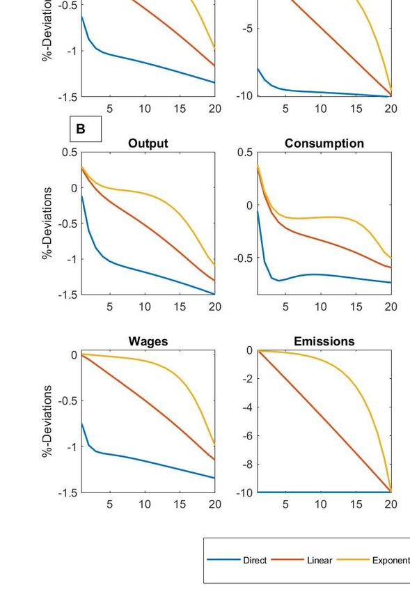
10% emission reduction relative to the no-policy scenario. If not indicated differently, the dynamics are
illustrated in terms of percentage deviations from the deterministic steady state over a horizon of 20
quarters.
Figure 1: Impulse responses of macroeconomic aggregates to TFP shock, in percentage deviations from
steady state. The underlying parameter values correspond to table 2.
Figure 1 depicts the dynamics in response to a one standard deviation increase in TFP. First, we
observe that emissions policies do not qualitatively alter the reaction of macroeconomic aggregates in
response to an increase in TFP. The innovation in productivity leads to a persistent increase in output,
consumption and investment. Due to the increased productivity, firms’ marginal costs fall. In the model,
because of price rigidities, firms cannot adjust their prices in accordance with the decline in marginal costs.
Therefore, the responses of aggregate demand for intermediate goods and consequently aggregate output
are dampened. In this situation firms adjust factor inputs in order to utilize the increased productivity.
Here, despite the increase in wages, which due to the presence of nominal wage rigidities displays a
hump-shaped pattern, aggregate working hours decline. This decline in response to the shock is essentially
16a feature of empirical data as emphasized by Gali (1999). Since investment is subject to convex adjustment
costs the increase in productivity causes a decline in the real interest rate on impact. In addition, investment
also displays a hump-shaped pattern.
Overall, there appear to be no qualitative difference in the reaction of macroeconomic aggregates
across policy instruments, but we observe quantitative differences in the model dynamics. In general,
under the price instruments, aggregate dynamics are most pronounced, whereas the dynamic is least
pronounced with a cap-and-trade system. The dynamics of emissions and emission prices display notable
differences between all instruments. While under the cap-and-trade scheme emissions do not react, they
increase under the intensity target and decrease in the case of price instruments. With an intensity target,
the amount of emissions permits increases with output, which leads to a decline in the permit price and
induces firms to increase the utilization of polluting inputs. In contrast with a constant price of emissions,
firms have no incentive to increase the amount of polluting inputs on impact. After a while, good prices
can adjust and emissions start to increase in proportion to the increase in the other input factors. Under a
flexible price regime, the same effects occur, but emission dynamics are dampened due to adjustments in
the price of emissions. The largest increase in the emissions price arises with a cap-and-trade regime. In
response to the shock, firms demand for the polluting input factor declines, which is reflected in a decline
in the market price of permits. In later periods, price adjustments take place and increase the demand for
intermediate goods, which induces firms to further expand production and spurs firms’ demand for input
factors. Now, with the strict cap on emissions, firms cannot increase intermediate inputs due to a lack
of permits. Here, the binding of the emissions constraint is associated with the largest price increase in
emissions. Under the other instruments, the amount of emissions is, at least to some extent flexible, which
allows quantity adjustments.
Figure 2 depicts the aggregate dynamics in response to a one standard deviation increase in government
expenditures. Under the given parameter values for the government sector, the additional government
expenditures are mostly financed through an increase in government debt. The increase of aggregate
demand, associated with the increase in government consumption, then leads to a jump of output and
aggregate consumption, and at the same time crowds out private investment. The crowding out of
investment is caused by Ricardian households, who increase their holdings of government bonds. Many
studies report a decline in aggregate consumption in response to government spending shocks. Here, as
explained by Galı́ et al. (2007), the initial increase in aggregate consumption results from the presence
of non-Ricadian households who have a marginal propensity to consume equal to one. Due to the
increase in hours and wages, their income increases, which directly translates into an increase in aggregate
consumption. Again, we observe that the policy instruments have quantitative implications for aggregate
dynamics and generally alter the responses. We observe that under a cap-and-trade system the dynamics
are stronger compared to the other policy regimes. This is particularly evident in the case of marginal
costs, which react much stronger under the cap-and-trade scheme. The constant price instrument results in
the smallest increase in consumption, marginal costs, hours and wages. In terms of magnitude, the effects
under the intensity target are somewhere between the price instruments and the cap-and-trade scheme.
The different effects of the instruments can be explained by their effects on the utilization of polluting
intermediate inputs through the emissions price. While under the constant price regime, emissions show
the strongest increase, and the increase is dampened under the flexible price regime and the intensity target.
As can be inferred from the dynamics of the emissions price, the government spending shock causes the
17You can also read