Photometric classification of HSC transients using machine learning
←
→
Page content transcription
If your browser does not render page correctly, please read the page content below
Publ. Astron. Soc. Japan (2020) 00(0), 1–23   1
                                                                                                                             doi: 10.1093/pasj/xxx000

                                               Photometric classification of HSC transients
                                               using machine learning
arXiv:2008.06726v1 [astro-ph.IM] 15 Aug 2020

                                               Ichiro TAKAHASHI1,2,4,* , Nao S UZUKI1 , Naoki YASUDA1 , Akisato K IMURA3 ,
                                               Naonori U EDA3 , Masaomi TANAKA4,1 , Nozomu TOMINAGA5,1 , and Naoki
                                               YOSHIDA1,2,6,7
                                               1
                                                 Kavli Institute for the Physics and Mathematics of the Universe (WPI), The University of
                                                 Tokyo Institutes for Advanced Study, The University of Tokyo, 5-1-5 Kashiwanoha, Kashiwa,
                                                 Chiba 277-8583, Japan
                                               2
                                                 CREST, JST, 4-1-8 Honcho, Kawaguchi, Saitama 332-0012, Japan
                                               3
                                                 NTT Communication Science Laboratories, 2-4 Hikaridai, Seika-cho, Keihanna Science City,
                                                 Kyoto 619-0237, Japan
                                               4
                                                 Astronomical Institute, Tohoku University, Aoba, Sendai, Miyagi 980-8578, Japan
                                               5
                                                 Department of Physics, Faculty of Science and Engineering, Konan University, 8-9-1
                                                 Okamoto, Kobe, Hyogo 658-8501, Japan
                                               6
                                                 Department of Physics, Graduate School of Science, The University of Tokyo, 7-3-1 Hongo,
                                                 Bunkyo-ku, Tokyo 113-0033, Japan
                                               7
                                                 Institute for Physics of Intelligence, The University of Tokyo, 7-3-1 Hongo, Bunkyo-ku, Tokyo
                                                 113-0033, Japan
                                               ∗ E-mail:   ichiro.takahashi@astr.tohoku.ac.jp
                                               Received hreception datei; Accepted hacception datei

                                               Abstract
                                               The advancement of technology has resulted in a rapid increase in supernova (SN) discoveries.
                                               The Subaru/Hyper Suprime-Cam (HSC) transient survey, conducted from fall 2016 through
                                               spring 2017, yielded 1824 SN candidates. This gave rise to the need for fast type classification
                                               for spectroscopic follow-up and prompted us to develop a machine learning algorithm using a
                                               deep neural network (DNN) with highway layers. This machine is trained by actual observed
                                               cadence and filter combinations such that we can directly input the observed data array into
                                               the machine without any interpretation. We tested our model with a dataset from the LSST
                                               classification challenge (Deep Drilling Field). Our classifier scores an area under the curve
                                               (AUC) of 0.996 for binary classification (SN Ia or non-SN Ia) and 95.3% accuracy for three-
                                               class classification (SN Ia, SN Ibc, or SN II). Application of our binary classification to HSC
                                               transient data yields an AUC score of 0.925. With two weeks of HSC data since the first
                                               detection, this classifier achieves 78.1% accuracy for binary classification, and the accuracy
                                               increases to 84.2% with the full dataset. This paper discusses the potential use of machine
                                               learning for SN type classification purposes.
                                               Key words: supernovae: general — methods: statistical — surveys

                                               c 2020. Astronomical Society of Japan.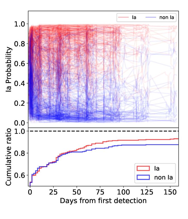
2                                                            Publications of the Astronomical Society of Japan, (2020), Vol. 00, No. 0

1 Introduction                                                    chine learning (DNN) to the actual transient survey data.
                                                                  The Hyper Suprime-Cam (HSC) (Miyazaki et al. 2018;
Time domain science has become a major field of astro-
                                                                  Komiyama et al. 2018; Kawanomoto et al. 2018; Furusawa
nomical study. The discovery of the accelerating universe
                                                                  et al. 2018), a gigantic mosaic CCD still camera mounted
(Perlmutter et al. 1999; Riess et al. 1998) evoked a series
                                                                  on the 8.2 m Subaru Telescope, makes it possible to probe
of large supernova (SN) surveys in the last few decades
                                                                  a wide field (1.77 deg2 field of view) and deep space (26th
(Betoule et al. 2014; Scolnic et al. 2018; Brout et al. 2019).
                                                                  mag in the i−band / epoch). Our primary scientific goals
These surveys revealed that an entirely new family of tran-
                                                                  are SN Ia cosmology, Type II supernova (SN II) cosmol-
sients exists and the search for unknown populations is cur-
                                                                  ogy, and super-luminous supernova (SLSN) studies as well
rently of great interest (Howell et al. 2006; Phillips et al.
                                                                  as to probe unknown populations of transients. As re-
2007; Quimby et al. 2007). For precision cosmology, it is
                                                                  ported recently Yasuda et al. (2019), more than 1800 SNe
highly important to maintain the purity of Type Ia super-
                                                                  were discovered during a 6-month campaign. We deployed
novae (SNe Ia) while performing uniform sampling of these
                                                                  machine learning (AUC boosting) for transient detection
SNe ranging from bright to faint. Spectroscopic follow-
                                                                  (Morii et al. 2016), where the machine determines whether
up has been essential to distinguish a faint SN Ia from
                                                                  a transient is “real” or “bogus.” In Kimura et al. (2017),
a Type Ib supernova (SN Ib) and a Type Ic supernova
                                                                  we adopted a DNN for SN type classification from a two-
(SN Ic) which have similar light curve behavior (Scolnic
                                                                  dimensional image, and highway block was introduced for
et al. 2014). Considering that a large amount of precious
                                                                  the optimization of layers. This research is an extension
telescope time is dedicated to these follow-up programs, it
                                                                  of our previous work Kimura et al. (2017) and applies a
is desirable to make efficient use of these telescopes.
                                                                  DNN to the photometric classification of transients. We
   The scale of surveys is becoming larger, and it has be-        uniquely attempt to use the observed data in a state that
come impossible to trigger spectroscopic follow-up for all of     is as “raw” as possible to enable us to directly use the
the candidates in real time. It has therefore become neces-       data as input for the machine without fitting the data or
sary to develop a new classification scheme, and a natural        extracting characteristics.
path along which to proceed would be to perform photo-
                                                                     The structure of this paper is as follows. We intro-
metric classification (Sako et al. 2011; Jones et al. 2018).
                                                                  duce our methods in section 2, and the data in section
The rise of machine learning technologies has resulted in
                                                                  3. The design of our DNN model and its application to
astronomical big data commonly being analyzed by using
                                                                  pseudo-real LSST simulation data is described in section
machine learning techniques.
                                                                  4. Section 5 presents the application of our model to the
   Neural networks have been used for photometric red-            actual Subaru/HSC data. We discuss the results in section
shift studies from the early stages. Today, many Machine          6 and conclude the paper in section 7.
Learning methods are applied to the photometric red-
shift studies (Collister & Lahav 2004; Carliles et al.
2010; Pasquet et al. 2019). Deep neural networks (DNNs)           2 Methods
are being used to process imaging data to identify strong
                                                                  2.1 Tasks in HSC survey
lens systems (Petrillo et al. 2017) or for galaxy morphol-
ogy classifications (Hausen & Robertson 2019). Currently,         The Subaru HSC Transient Survey forms part of the
machine learning is being introduced to process tran-             Subaru Strategic Project (SSP), which is a five-year pro-
sient survey data for detection (Goldstein et al. 2015)           gram with a total of 300 dark nights (Aihara et al.
and classification purposes (Charnock & Moss 2017). A             2018a; Miyazaki et al. 2018). The HSC-SSP Transient
recurrent autoencoder neural network (RAENN) is in-               Survey is composed of two seasons, the first of which was
troduced for photometric classification of the SN light           executed for six consecutive months from November 2016
curves (Villar et al. 2020), and being applied to 2315            through April 2017. The HSC is mounted on the prime
Pan-Starrs1 data (Hosseinzadeh et al. 2020). In prepa-            focus for two weeks in dark time. Weather permitted, we
ration for the Vera C. Rubin Observatory, a real time             aimed to observe two data points per filter per lunation.
classifier, ALeRCE (Automatic Learning for the Rapid              Details of the survey strategies and the observing logs were
Classification of Events), is being developed (Sánchez-Sáez     reported in Yasuda et al. (2019), and we used the observed
et al. 2020; Förster et al. 2020) and currently applied to       photometric data described in Yasuda et al. (2019).
the Zwicky Transient Facility (ZTF) data (Carrasco-Davis            One of our primary goals with the HSC-SSP Transient
et al. 2020).                                                     Survey is SN Ia cosmology which aims to perform the
    In this paper, we introduce our attempt to apply ma-          most precise measurement of dark energy at high-redshift
Publications of the Astronomical Society of Japan, (2020), Vol. 00, No. 0                                                         3

and test whether the dark energy varies with time (Linder                  An early phase SN Ia provides us with clues on the
2003). We have been awarded 96 orbits of Hubble Space                   explosion mechanism (Maeda et al. 2018) and progenitors
Telescope time (WFC3 Camera) to execute precise IR pho-                 (Cao et al. 2015). The advantage of HSC is its ability to
tometry at the time of maximum. Our HST program uses                    survey a large volume, and in practice, it has confirmed the
non-disrupted ToO, which means we are required to send                  long-standing theoretical prediction of helium-shell deto-
the request for observation, two weeks prior to the observa-            nation (Jiang et al. 2017). Finding early phase SN Ia is
tion. In other words, we need to identify good candidates               not trivial but HSC is yielding a new set of early phase
2–3 weeks prior to the maximum. Although a high-redshift                SN Ia (Jiang et al. 2020). Observations of early phase core-
(z > 1) time dilation factor helps, it is always a challenge            collapse SNe provide us with crucial information on the size
to identify SN Ia on the rise.                                          of the progenitors (Thompson et al. 2003; Tominaga et al.
   Our international collaboration team executes spectro-               2011) and Circumstellar Medium (Förster et al. 2018).
scopic follow-up using the large telescopes in the world.
Our target, high-redshift SN Ia, is faint (∼ 24th mag
                                                                        2.2 Classification method for HSC-SSP transient
in the i−band) for spectroscopic identification even with
                                                                            survey
the most powerful large telescopes: GMOS Gemini (Hook
et al. 2004), GTC OSIRIS,1 Keck LRIS (Oke et al. 1995),                 We designed two machine learning models with the empha-
VLT FORS (Appenzeller et al. 1998), Subaru FOCAS                        sis on identifying SN Ia, which requires a time-sensitive
(Kashikawa et al. 2002) and AAT AAOmega Spectrograph                    trigger for HST IR follow-up. The first model operates
(Saunders et al. 2004). Thus, it is critical to hit the target          in binary mode and classifies whether a transient is of
at the time of maximum brightness either by using ToO                   the SN Ia. In this regard, the majority of high-redshift
(GTC), queue mode (VLT) or classical scheduled observa-                 transients are known to be of the SN Ia type, and our
tion (Keck, Subaru, ATT).                                               work entails searching for other unknown transients from
   A SN Ia requires approximately 18 days from its ex-                  among those labeled non-SN Ia. The second model clas-
plosion to reach its maximum in rest frame (Conley et al.               sifies a transient into one of three classes: SN Ia, SN Ibc,
2006; Papadogiannakis et al. 2019). Given this fact, the                or SN II. These three classes were chosen for simplicity
SNe with which we are concerned is high-redshift SN Ia                  and in fact, the majority of SNe belong to one of these
(z > 1), in which case we have approximately one month                  three categories. SN Ia is a thermonuclear explosion, and
in the observed frame for a SN Ia from the time of explo-               its brightness can be calibrated empirically. SN Ib, SN Ic,
sion until it reaches its maximum. However, our task is to              and SN II are all core-collapse SNe and are classified by
identify these SNe two weeks prior to the maximum, which                their spectral features (Filippenko 1997). The light curves
means we have only two data points per filter. In addition              of SN Ib and SN Ic, which are collectively referred to as
to that, the sky conditions continue to change, and we                  SN Ibc, are similar to those of SN Ia and always contami-
may not have the data as originally planned. In reality,                nate the SN Ia cosmology program. They are fainter than
our identification has to proceed despite data points being             SN Ia and redder in general. A major challenge of this
missing on the rise.                                                    work is to determine whether we can distinguish SN Ibc
   In parallel to the SN Ia cosmology program, our sis-                 from SN Ia.
ter projects also need identification and classification of
HSC transients. Specifically, the SN II cosmology pro-
gram requires timely spectroscopic follow-up to measure
                                                                        3 Data
the expansion velocity of photosphere from the Hβ line                  In this section, we present the dataset we used for our
(de Jaeger et al. 2017). A SLSN is of great interest to-                study. We first introduce our SN dataset from the HSC-
day, because it is a relatively rare event (Quimby et al.               SSP Transient Survey (subsection 3.1). Then we describe
2011) and its mechanism has quite a diversity (Gal-Yam                  the simulated photometric data to train the machine (sub-
2012; Moriya et al. 2018), and it can be used to probe                  section 3.2). Lastly, we explain the pre-processing of the
the high-redshift Universe (Cooke et al. 2012). New types               above data for input into the machine (subsection 3.3).
of rapid transients are also discovered by HSC, but their
identities are yet to be known (Tampo et al. 2020). For
these projects, timely spectroscopic follow-up is also criti-
                                                                        3.1 Observed data from Subaru/HSC-SSP transient
                                                                            survey
cal (Moriya et al. 2019; Curtin et al. 2019).
                                                                        The goal of this project is to classify the light curves
1
    GTC OSIRIS hhttp://www.gtc.iac.es/instruments/osiris/i.             observed by Subaru/HSC. The discovery of 1824 SNe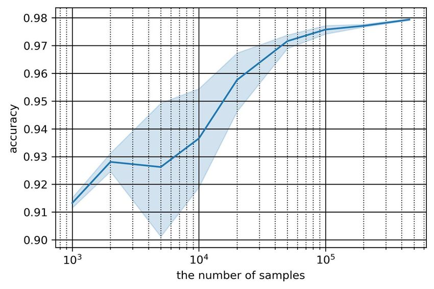
4                                                           Publications of the Astronomical Society of Japan, (2020), Vol. 00, No. 0

recorded during the six-month HSC-SSP Transient Survey           mology with Ωm =0.3 and h=0.7. We used the filter re-
during the period of November 2016 through April 2017            sponse including system throughput from Kawanomoto
was reported and described in Yasuda et al. (2019). The          et al. (2018). Examples of simulated photometric data are
survey is composed of the Ultra-Deep and Deep layers in          shown in figure 1.
the COSMOS (Scoville et al. 2007). The median 5σ lim-               A complication that arises when attempting to simulate
iting magnitudes per epoch are 26.4, 26.3, 26.0, 25.6, and       realistic data is that the machine does not accept expected
24.6 mag (AB) for the g-, r2-, i2-, z- and y-bands, respec-      errors. Alternatively, we may not have identified a good
tively, for the Ultra-Deep layer. For the Deep layer, the        method for including errors. In this study, we therefore
depth is 0.6 mag shallower.                                      simply used brute force, namely, we placed the expected
    The SN dataset consists of time series photometric data      photometric error on top of the simulated data such that a
(flux, magnitude, and their errors) in each band for each        simulated data point behaves similarly to one of the many
SN. Because part of the y-band photometric data contains         realizations. The magnitude of the error in the HSC sim-
residuals due to improper background subtraction influ-          ulation would have to consider varies from night to night
enced by scattered light (Aihara et al. 2018b), we excluded      because of sky conditions. We measured and derived the
the y-band data from our study, considering the impact           flux vs. error relationship from the actual observed data
thereof on the classification performance.                       at simulating epoch and applied that relationship to the
   The redshift information for HSC SNe is a combina-            simulated photometric data.
tion of our follow-up observation results and catalogs from         Guided by the “accuracy” (subsection 4.2), we de-
multiple surveys of those host galaxies. The spectral red-       termined the number of light curves that would be re-
shifts (spec-z) are adopted from the results of the follow-up    quired for training. Based on our convergence test, we
spectrum observations by AAT/AAOmega performed in                concluded that we would need to generate more than
2018 and those from the DEIMOS (Hasinger et al. 2018),           100,000 light curves for training as shown figure 2. We
FMOS-COSMOS (Silverman et al. 2015), C3R2 (Masters               omitted the curves with less than 3σ detection at the
et al. 2017), PRIMUS (Coil et al. 2011) and COSMOS cat-          maximum because our detection criterion was 5σ. For
alogs. For those without spec-z, the photometric redshifts       training, we generated 514,954 light curves for HSC ob-
(photo-z) were adopted from the COSMOS 2015 catalog              served data. Their final class ratio after these criteria
(Laigle et al. 2016) and those calculated from the HSC-          is SN Ia:Ibc:II=0.59:0.07:0.34, and their peak timings are
SSP survey data (Tanaka et al. 2018).                            randomly shifted by 450 days.

3.2 Simulated data for training                                  3.3 Preprocessing of input data
                                                                 Based on our pre-experiment with the simulated dataset,
We are in need of simulating observed photometric data to
train the machine. For normal SN Ia, we used the SALT2           we found the machine to perform best by using a com-
(Guy et al. 2010) model (ver 2.4) that requires two input        bination of the normalized flux (f ) and pseudo-absolute
parameters: c for color and x1 for stretch. We adopted           magnitude (M ):
                                                                                                                         T
an asymmetric Gaussian distribution for c, and x1 from           x = M1abs , . . . , MPabs , f1scale , . . . , fPscale        ,   (1)
Mosher et al. (2014), and generated light curves and sim-
ulated photometric data points based on the observation          where fiscale is the i-th raw observed flux normalized by its
schedule. Apart from SN Ia, we used published spectral           maximum flux:
time series from Kessler et al. (2019) which contains both                         fi
                                                                 fiscale =                          ,                             (2)
observed Core-Collapse SN data and light curves from the                     max (f1 , . . . , fP )
simulation. We combined an equal number of SN Ia and             and Miabs is the i-th pseudo-absolute observed magnitude.
non-SN Ia observations to approximate the observed frac-         For simplicity, we ignored K-correction and used the dis-
tions. Although these fractions do not need to be exact for      tance modulus (DM(z)) based on ΛCDM with the photo-
the purpose of our classification, it is important to avoid      metric redshift from its host galaxy.
using an unbalanced dataset. For three class classification,
                                                                 Miabs = mi − DM (z) ,                                            (3)
we set the ratio of SN Ia:SN Ibc:SN II=10:3:7. The redshift
distribution of galaxies was taken from the COSMOS sur-          We can justify this operation because the training set and
vey (Laigle et al. 2016), and we distributed the simulated       the observed dataset are processed using the same ap-
SNe accordingly from z =0.1 through z =2.0. Throughout           proach. In the case of the existence of K-correction offset,
the study reported in this paper, we used ΛCDM cos-              both datasets would experience this in the same way. In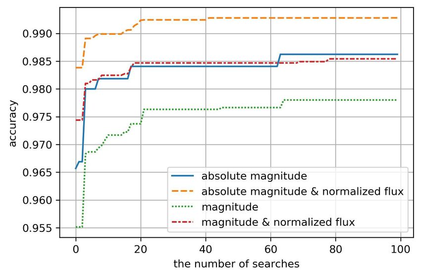
Publications of the Astronomical Society of Japan, (2020), Vol. 00, No. 0                                                                                       5

Fig. 1. Overlay plots of simulated light curves with z between 0.1 and 1.2. Each panel shows the plots of SN Ia, Ibc, II data from the left, and the g-, r2-, i2-,
z-, y-bands from the bottom. The variation of the curves in each panel depends on the different parameters and templates used in the simulation. A noise
component was not added to these light curves.
6                                                                           Publications of the Astronomical Society of Japan, (2020), Vol. 00, No. 0

                                                                                 color, the width of the light curve, and the peak magnitude.
                                                                                    The fact that we went one step further by leaving the
                                                                                 observed data as raw as possible, means that our input
                                                                                 consists of a simple array of magnitudes. An attempt such
                                                                                 as this would not have been possible ten years ago; how-
                                                                                 ever, owing to advancements in computing and the deep
                                                                                 learning technique, this has become reality. Among the
                                                                                 many machine learning methods, we decided to use a DNN
                                                                                 to enable us to classify astronomical objects from the raw
                                                                                 observed data.

                                                                                 4.1 Model design
Fig. 2. Convergence test to determine the number of light curves that would      In this section, we describe the design of our DNN model,2
need to be generated to train the machine. The solid line shows the mean
                                                                                 which accepts an array of observed magnitudes as its in-
accuracy of five classifiers. The shaded area shows the standard deviation
of the classifiers, which were trained with 5-fold cross validation using the    put and outputs the SN classification with probabilities.
training dataset. The results indicate that more than 100,000 light curves       We adopted a highway layer (also known as a “layer in
would be required for training.                                                  layer”, Srivastava et al. 2015a) as a core part of our net-
                                                                                 work. Compared to plain DNN, the performance of a high-
addition, because the observed flux could take on a nega-                        way layer improves when the network is deep in terms of
tive value owing to statistical fluctuation, we adopt hyper-                     parameter optimization (Srivastava et al. 2015b).
bolic sine to imitate the magnitude system we use (Lupton                            Similar to other DNN models, this model proceeds
et al. 1999).                                                                    through a training and validation process to optimize the
                  2.5        fi                                                  parameters, and we describe the steps below. Our termi-
mi = 27.0 −            sinh−1 .                                          (4)     nology is commonly used in the world of DNN, but as this
                log 10       2
In fact, combination of the flux and magnitudes is redun-                        is a new introduction to the astronomical community, we
dant, because knowledge of the one would enable us to                            explain each step in detail. The architecture of our model
calculate the other explicitly. However, based on our ex-                        is summarized in figure 3. Ultimately, each SN is assigned
periment, the score of the machine improves by using both.                       a probability of belonging to a certain astrophysical class,
We suspected that the distribution in flux (linear) differs                      in our case, the type of SN.
from that of the magnitude space (log), which provides the                           Input: Our input is an array of magnitudes and nor-
machine with additional information. Thus, we used the                           malized fluxes of the ith SN in the training dataset:
pseudo-absolute magnitude (M ) and normalized flux (f )                          xi = (Mi1 , Mi2 , . . . Mij . . . , MiN , fi1 , fi2 , . . . , fiN )T   (5)
as an input.
                                                                                 We do not explicitly specify the time at which or the par-
                                                                                 ticular filter with which the data were recorded, but this
4 Deep neural network classifier                                                 information is recorded as an order inside the array. The
With the rise of Big Data, the use of machine learn-                             philosophy here is that the training set, which is composed
ing techniques has played a critical role in the analy-                          of simulated data of the same array length, holds informa-
sis of astronomical data. Techniques such as random                              tion on the filter and dates. For example, the jth magni-
forest, support vector machine, and convolution neural                           tude in the array is data recorded on a certain date and
network have been used for photometric data analysis                             by a certain filter. The combination of the date and filter
(Pasquet et al. 2019), galaxy classifications (Hausen &                          is identical to those in the training set. Therefore, the jth
Robertson 2019), and spectral classifications (Garcia-Dias                       component implicitly contains unique information about
et al. 2018; Muthukrishna et al. 2019b; Sharma et al. 2020).                     the dates and filters. Considering that the input consists
                                                                                 of a combination of the magnitude and normalized flux,
   In our work, we seek to classify SNe from photometric
data. Our approach entails making use of the observed                            the size of our input array is 1 × 2N per SN where N is
data without pre-processing or parameterization. In this                         the number of data points.
regard, we rely on deep learning to make our work possible.                          First Fully Connected layer: We decided to make
We decided to test the extent to which deep learning could                       2
                                                                                     The code for our model is available at hhttps://github.com/ichiro-
provide useful results without extracting features such as                           takahashi/snclassi.
Publications of the Astronomical Society of Japan, (2020), Vol. 00, No. 0 7 Fig. 3. Architecture of the deep neural network classifier. The green boxes are parameters optimized by the gradient descent method during training. The red boxes are hyperparameters that are optimized during the hyperparameter search. The batch normalization layer has four variables (µ, σ2 , γ, β), where µ and σ2 are intended to learn the statistics (mean and variance) of the value through the layer, respectively, and γ and β are scale and shift parameters, respectively, to adjust the output. Note that µ and σ2 are not updated by gradient descent; instead, they are updated by the moving average. They were omitted from the figure for simplicity.
8                                                            Publications of the Astronomical Society of Japan, (2020), Vol. 00, No. 0

use of D neurons, also known as the number of “hidden             Highway (x) = G (x) ⊗ H (x) + C (x) ⊗ x ∈ RD ,                  (7)
layers,” and D is greater than the number of input com-
                                                                  where H is a nonlinear transformation layer, G is the trans-
ponents (2N ). However, the dimension of D is not known
                                                                  formation gate function layer and controls the transfor-
in advance, and this is one of the hyperparameters we op-
                                                                  mation of input, C is the carry gate function layer, and
timize later in this section. Because the dimensionality of
                                                                  ⊗ provides the element-wise product, also known as the
the input (2N ) could differ from the number of optimized
                                                                  Hadamard product. A highway layer includes several other
neurons D, we would need to adjust the number of dimen-
                                                                  layers, a structure known as “layer in layer.” Each function
sions and that is the role of this first fully connected layer
                                                                  is defined as follows:
F (x).
                                                                                                              ∈ RD ,

                                                                  H (x) = a F x, WHf c , bHf c                                    (8)
F (x, {Wf c1 , bf c1 }) = Wf c1 x + bf c1 ∈ RD .          (6)
                                                                                                                 D

                                                                   G (x) = a F x, WGf c , bGf c               ∈R ,                (9)
F (x) is given by a linear combination of matrix Wf c ∈                                       D
                                                                   C (x) = 1 − G (x) ∈ R ,                                       (10)
RD×2N and a vector bf c ∈ RD . The initial value of Wf c
is generated by Gaussian distribution and bf c is initialized     where a is an activation function, namely, sigmoid.
by 0, which is a D-dimensional vector of which all the
                                                                   a (p) = (σ (p1 ) , σ (p2 ) , . . . , σ (pD ))T , p ∈ RD ,
elements are zero. We used the Python wrapper library                          1
dm-sonnet 3 (version 1.23) and its function linear to supply      σ (pi ) =            ,
                                                                            1 + e−pi
the F (x) when plugging in “2N ” and “D.” Subsequently,           where D is the number of neurons. Each element of G(x)
Wf c and bf c are optimized by the open source machine-           always takes a value between 0 and 1. Eventually, the
learning package Tensorflow (version 1.14) (Abadi et al.          Highway layer behaves as follows:
2016). Unless stated otherwise, we used the libraries from
                                                                                           x,       if G (x) = 0
Tensorflow.                                                       Highway(x) =                                                   (11)
                                                                                           H(x),    if G (x) = 1
   Dropout layer: To obtain a robust result, it is always
best to train all of the neurons as an ensemble and avoid a       Along with the dimensions of the hidden layer D, the
situation in which one of the neurons adversely affects the       dropout ratio, batch normalization, and the types of ac-
result. Dropout is a process in which certain neurons are         tivation function, the number of repetitions T is one of
randomly dropped from training and the dropout rate can           the hyperparameters and is optimized by performing a hy-
be optimized as one of the hyperparameters (Srivastava            perparameter search. Details are provided in subsection
et al. 2014).                                                     4.2.
    Highway layer: We adopted a Highway layer                         Batch Normalization layer: We adopt batch nor-
(Srivastava et al. 2015a) and optimized the number of lay-        malization (Ioffe & Szegedy 2015) to accelerate and stabi-
ers therein during the hyperparameter search. In theory, it       lize the optimization. Even if a large number of parameters
would be possible to design a very deep layer with more lay-      need to be trained, batch normalization facilitates conver-
ers than would be necessary. However, in reality, it is not       gence of the training process, reduces errors on the slope
trivial to optimize the number of layers. The depth and/or        when we apply entropy minimization, prevents the aver-
size of the layers of the DNN model are directly related to       age and dispersion from becoming exponentially large in
the complexity of the features used as input, and greatly         deep layers, and minimizes the biases on outputs (Bjorck
affect the computational performance of the task. Thus,           et al. 2018). Batch normalization is effective in many cases.
an overly deep model would complicate the learning pro-           However, the performance of a model that employs both
cess and cause performance degradation. A highway layer           batch normalization and dropout may degrade (Li et al.
is a technique that stabilizes the learning process by devis-     2019).
ing the network structure. We previously used a highway               Activation layer: Each neuron is activated by using
layer, which we tested on 2D images, and it delivered good        nonlinear transformation. Nonlinearity is an important
performance (Kimura et al. 2017). Details of the use and          component of DNN, because it allows a wide variety of ex-
advantages of the highway layer are provided in Kimura            pressions. Note that the majority of the layers, including
et al. (2017). This encouraged us to adopt a highway layer        fully connected layers, involve a linear transformation and,
scheme for this analysis. The output of the highway layer is      even if a number of layers were to exist, it would be equiv-
calculated from the values of multiple paths. The output,         alent to one single linear transformation. Thus, nonlinear
Highway (x), is formulated as                                     transformation is essential to allow each neuron the free-
                                                                  dom to have any necessary values. For the first iteration,
3
    dm-sonnet hhttps://github.com/deepmind/sonneti.               we do not know what kind of transformation is the best;
Publications of the Astronomical Society of Japan, (2020), Vol. 00, No. 0 9
thus, the transformation itself is taken as one of the hyper- Table 1. Ranges of hyperparameter search for Type
parameters. In our work, we used the functions “tf.nn,” in Classification
Tensorflow. hyper parameter value (grid) range (TPE)
Second Fully Connected layer: After T repetitions D {100, 300} 50, . . . , 1000
of the highway layer, batch normalization layer, and ac- T {1, 3, 5} 1, . . . , 5
tivation layer, it is necessary to convert the number of bn {true} {true, false}
drop rate [5e-3, 0.035] [5e-4, 0.25]
neurons to the number of SNe times the number of SN
type {identity, relu, sigmoid, tanh}
classes. This operation is opposite to that of the first fully
connected layer.
Softmax layer: The Softmax layer normalizes the in-
put value of this layer, which is denoted by h ∈ RD . The
output value is ŷ ∈ RD and each element ŷk is expressed as
exp (hk )
ŷk = PK . (12)
k′ =1
exp(hk′ )
PK
The normalized value ŷ satisfies ŷk ≥ 0 and k
ŷk = 1.
We can interpret ŷk as the probability that the input x
belongs to class k. However, we note that this is a pseudo-
probability and that it differs from the statistical proba-
bility.
4.2 Hyperparameter search Fig. 4. Result of iterative hyperparameter search (100 cycles) showing its
convergence to its maximum performance in terms of accuracy. The task
We perform a hyperparameter search by combining grid involved binary classification.
search and the Tree-structured Parzen Estimator (TPE)
algorithm (Bergstra et al. 2013). Although grid search
also three. In binary classification (SN Ia or non-SN Ia),
is not suitable to search a high-dimensional space, it has
the number of outputs is two.
the advantage of searching for multiple points in parallel.
We trained the model by minimizing the cross-entropy
In addition, because of the simplicity of the algorithm, it
error:
allows us to convey knowledge acquired during preliminary
K
experiments for parameter initialization. Meanwhile, the X
CE (y, ŷ) = − yk log ŷk , (13)
TPE algorithm is suitable for searching a high-dimensional k=1
space, but has the disadvantage of not knowing where to
where y is the ground truth vector, which entails one-hot
start initially. Therefore, this time, our search was guided
encoding of K dimensions, and ŷ is the DNN output vector.
by the hyperparameter values that were obtained in the
We deployed the Adam optimizer (Kingma & Ba 2014)
preliminary experiment using grid search, and these results
which uses a stochastic gradient method to optimize the
were then used as input for the TPE algorithm. The ranges
model parameters.
in which we searched for the hyperparameters are given in
We introduced data augmentation to prevent overfitting
table 1.
at the time of training. By increasing the number of input
According to the usual approach, we divided the dataset data by using data augmentation, we prevent DNN from
into training and validation datasets. We used the training having to memorize the entire training dataset. We used
data to optimize the DNN, and the validation data to mea- two data augmentation methods to augment the training
sure the accuracy. The hyperparameters were optimized dataset. The first was to add Gaussian noise (based on the
by evaluation with the validation dataset to maximize the expected observed uncertainty) to the simulated flux. The
accuracy of this dataset. This process was iteratively con- second involved the use of the mixup technique (Zhang
ducted 100 times to allow the accuracy to converge to its et al. 2017).
maximum (figure 4). Mixup generates a new virtual training dataset as fol-
We can train the DNN classifier in the same way re- lows:
gardless of the number of classes. In the case of multi-type
classification, the number of classes is K = 3 in our experi- x̃ = λxu + (1 − λ) xv ,
ment; thus, the number of outputs of the DNN classifier is ỹ = λyu + (1 − λ) yv ,10 Publications of the Astronomical Society of Japan, (2020), Vol. 00, No. 0
where (xu , yu ) and (xv , yv ) are samples drawn at random spectively. Our investigation showed that a combination
from the training dataset, x is the input vector, y is the of the normalized flux (f ) and pseudo-absolute magnitude
one-hot label vector, and the mixing ratio λ ∈ [0, 1] is drawn (M ) performs best, and, although the information is re-
from a random distribution, of which the density is low dundant, we suspect the different distribution of the data
near 0 and 1 and higher near 0.5. The datasets generated provides the machine with additional guidance. The AUC
in this way are suitable to enable the DNN to learn the values for the ROC curve and the precision-recall curve are
classification boundaries. 0.996 and 0.995, respectively. Figure 5 shows the confu-
As described above, the hyperparameters (red boxes in sion matrix for the three-class classification, with the total
figure 3) of the model are optimized by maximizing the accuracy calculated as 95.3%. As is always the case in the
accuracy, whereas the model parameters (green boxes in real world, it is difficult to classify SN Ibc, but the effect on
figure 3) are optimized by minimizing the cross-entropy overall accuracy is relatively small. Table 3 summarizes
error.
Table 2. Classification performance of each input
for the PLAsTiCC dataset.
4.3 Testing the DNN model with PLAsTiCC dataset Input∗ AUC Accuracy
M m f ROC Pre.-Rec.
Before we applied our model to the data observed by HSC,
X X 0.996 0.995 0.953
we tested it with a dataset resulting from the LSST simu-
X 0.995 0.993 0.952
lated classification challenge, i.e., the PLAsTiCC dataset X X 0.995 0.993 0.948
(The PLAsTiCC team et al. 2018; Malz et al. 2019), which X 0.995 0.991 0.940
is composed of realistic photometric data with errors on ∗
Input to classifier is displayed as a check mark. M:
time-variable objects. To evaluate our model, we required pseudo-absolute magnitude, m: magnitude, f :
a dataset with labels of true identity. The PLAsTiCC Deep normalized flux.
Drilling Field (DDF) dataset contains data similar to those
in the HSC-SSP Transient Survey, and we took advantage
thereof. However, we generated the training set by our- Normalized confusion matrix
selves and selected not to use the training set provided Accuracy:0.953
by the PLAsTiCC team because we knew that the size of
Ia 0.96 0.01 0.03
their training dataset was insufficient to achieve maximum (964) (8) (28)
performance (figure 2).
True label
The training dataset was created by using the method
Ibc 0.06 0.74 0.20
described in subsection 3.2. We generated 370,345 light
curves based on the filter response and photometric zero-
(9) (119) (32)
point for LSST (Ivezić et al. 2019). These light curves
are composed of the different types of SNe in the ratio
II 0.02 0.01 0.97
SN Ia:Ibc:II=0.60:0.06:0.34, and their peaks are randomly (21) (9) (1107)
shifted in time. The test dataset was created by extracting
2,297 light curves from the PLAsTiCC dataset. These light Ia Ibc II
curves are labeled Ia, Ibc, or II, to identify the type of SN
Predicted label
each curve represented. The light curves were simulated
to occur in the COSMOS field. Fig. 5. Normalized confusion matrix in the three-class classification of the
PLAsTiCC dataset. The classifier received the pseudo-absolute magnitude
We used the area under the curve (AUC) of the receiver and normalized flux as its input. The proportions in each row sum to 1. The
operating characteristic (ROC) curve, the precision-recall numbers in parentheses represent the raw numbers.
curve in two-class classification, and the accuracy from the
confusion matrix in three-class classification as a metric the classification performance for each group of the test set
to evaluate our model. Different combinations of inputs divided according to the maximum signal-to-noise ratio of
were tested to determine which performs best when us- the photometric data. It shows that the classification per-
ing the PLAsTiCC dataset. Our input could be a com- formance tends to improve as the maximum signal-to-noise
bination of the arrays of normalized flux (f ), magnitude ratio increases.
(m), or the pseudo-absolute magnitude (M ). Table 2 lists In the three-class classification of the PLAsTiCC
the AUC for two-class classification and the accuracy for dataset, 107 SNe were misclassified and have the follow-
three-class classification when using PLAsTiCC data, re- ing characteristics:Publications of the Astronomical Society of Japan, (2020), Vol. 00, No. 0 11
Table 3. Classification performance for the 5 Application to HSC-SSP transient survey
maximum signal-to-noise ratio (SNR).
We applied the developed classifier to the dataset acquired
Max. SNR Number AUC∗ during the HSC-SSP Transient Survey. This dataset in-
ROC Pre.-Rec. cludes photometric data of 1824 SNe. As described in
20 716 0.999 0.999
All 2297 0.996 0.995
points of an SN in each layer could be different. Our DNN
∗
AUC for the best performing model (M + f ).
model requires exactly the same number of data points as
its input; thus, we divided our dataset into five cases based
on the number of photometric data points. The number
of SNe for each case is summarized in table 4. For exam-
• 54% (58/107) of them were “incomplete events” that did
ple, the number of SNe in Case 0 is 709, and they are in
not include the peak phase of the SN (the period of 10
the Ultra-Deep field. Each SN is represented by a total
days before and 20 days after the peak in the observed
of 42 epochs of photometric data in four bands (g-, r2-,
frame) in the photometric data, whereas they only con-
i2- and z-band). The number of epochs and filter schedule
stitute 38% of all events.
for Case 0 SNe are summarized in table 5. The introduc-
• Of the remaining misclassifications, 29% (14/49) are on
tion of these five cases enabled the machine to correctly
the boundary where the difference in probability be-
classify 1812 HSC SNe, which corresponds to 99.3% of the
tween the correct class and the predicted class is less
1824 SNe. The remaining 12 SNe were excluded owing
than 0.1.
to missing data. We subjected the aforementioned five
• In more than half of the remaining 35 events, SN Ibc
was misclassified as either SN Ia or II. Table 4. Number of SNe for each Case.
Case Epoch Number Fraction
Figure 6 shows the accuracy against redshift for the 0 42 709 0.391
PLAsTiCC dataset. The accuracy for SN Ibc is lower than 1 26 646 0.357
that of the other classes; in particular, it is greatly reduced 2 19 271 0.150
at redshifts beyond 1.0, and also decreased at redshift z of 3 10 122 0.067
4 4 64 0.035
0.1 to 0.2. Manual verification of individual misclassifica-
tions revealed that, although certain misclassified SNe are
too faint to classify even with conventional methods, a few Table 5. Number of input epochs and the schedule for
bright SNe were also completely misclassified. Case 0 SNe.
Filter Epochs Elapsed day
g 8 2, 40, 63, 70, 92, 119, 126, 154
r2 9 5, 32, 61, 71, 92, 103, 122, 129, 151
i2 13 2, 6, 32, 40, 61, 68, 71, 94, 101,
120, 127, 154, 155
z 12 0, 6, 30, 40, 59, 68, 90, 101, 119,
126, 151, 157
cases of observed HSC data to both two-class and three-
class classification. For each of these cases, the machine
needs to be trained independently with a dedicated train-
ing dataset. Thus, the hyperparameters were optimized for
each case and are reported in table 6. The following sub-
sections (subsection 5.1 and 5.2) describe the performance
evaluation for each classification.
Fig. 6. Accuracy as a function of the redshift in the three-class classification
of the PLAsTiCC dataset.
5.1 Binary classification
Binary classification was performed using four versions of
classifiers, which we prepared with different inputs as in the12 Publications of the Astronomical Society of Japan, (2020), Vol. 00, No. 0
Table 6. Optimized hyperparameters for classification
Input∗ Two-Class Three-Class
M m f T D drop rate bn type T D drop rate bn type
Case 0 X X 5 178 9.47e-3 1 sigmoid 4 429 1.20e-3 0 linear
X 3 247 9.68e-4 1 sigmoid 4 516 2.54e-3 0 tanh
X X 4 531 6.43e-3 0 linear 4 608 1.72e-2 0 linear
X 4 411 9.00e-2 1 sigmoid 4 838 1.36e-3 0 tanh
Case 1 X X 5 734 8.75e-4 0 tanh 4 915 1.03e-2 0 linear
X 2 389 7.17e-2 1 sigmoid 5 698 2.79e-2 0 linear
X X 2 647 7.92e-4 0 tanh 4 540 1.45e-3 0 linear
X 2 342 1.42e-2 1 sigmoid 2 520 9.99e-4 1 sigmoid
Case 2 X X 2 368 1.79e-3 1 sigmoid 4 698 9.08e-4 0 linear
X 4 920 1.44e-3 0 sigmoid 4 614 7.03e-3 0 linear
X X 5 572 4.27e-3 1 sigmoid 4 896 8.58e-3 0 linear
X 4 640 1.12e-1 1 sigmoid 5 300 5.00e-1 1 sigmoid
Case 3 X X 5 893 1.42e-3 1 sigmoid 4 522 5.02e-4 0 tanh
X 4 880 1.98e-2 1 sigmoid 5 841 4.96e-2 1 sigmoid
X X 3 300 5.00e-3 1 linear 3 462 9.28e-4 1 sigmoid
X 3 930 9.77e-2 1 sigmoid 3 300 5.00e-3 1 sigmoid
Case 4 X X 5 379 4.21e-3 1 sigmoid 3 484 2.13e-3 0 linear
X 2 631 1.77e-2 0 sigmoid 4 243 3.21e-3 1 sigmoid
X X 5 140 4.04e-3 1 sigmoid 5 389 1.23e-4 0 tanh
X 4 567 5.77e-2 0 sigmoid 3 354 2.14e-1 1 sigmoid
∗
Input to classifier is displayed as a check mark. M: pseudo-absolute magnitude, m: magnitude, f : normalized
flux.
PLAsTiCC dataset. This approach allowed us to compare of which the number of dof is five or more. The number
their performance, a summary of which is provided in table of labeled Ia, Ia?, and non-Ia are 429, 251, and 908 (410,
7. 240, and 850, with redshift), respectively. Apart from the
For the validation dataset, which is part of the simu- above, 215 SNe with less than 5 dof were labeled as “un-
lated dataset, a higher number of input dimensions were classified,” and the remaining 21 SNe failed to be fitted.
found to improve the results, enabling any classifier to clas- This performance evaluation was conducted by using 428
sify the data with very high AUC. The best AUCs for SNe Ia and 904 non-SNe Ia classified by our machine.
all classified events are 0.993 and 0.995 for the ROC and We also extracted 441 “light-curve verified SNe” that
precision-recall curve, respectively. have photometric information before and after their peak
For the test dataset, the classification performance was and for which spec-z are available, and verified their clas-
verified using 1332 HSC SNe (1256 with redshift) labeled sification results. Figures 7 and 8 show the AUCs of the
by the SALT2 light curve fitter (Guy et al. 2007; Guy et al. best classifier for all labeled HSC SNe and the light curve
2010), a conventional classification method. The verifica- verified HSC SNe respectively. The confusion matrices for
tion label for the HSC SNe conforms to that reported in each case are shown in figure 9. The best performing clas-
Yasuda et al. (2019), which defines SN Ia as SNe that sat- sifier obtained the same classification results as the con-
isfy all four of the following criteria for the SALT2 fitting ventional method for 84.2% of 1256 labeled SNe, which is
results: (1) color (c), and stretch (x1 ) within the 3σ range 91.8% accurate for the 441 light curve verified SNe.
of Scolnic & Kessler (2016) “All G10” distribution, (2) ab- In the binary classification of 1256 labeled HSC SNe,
solute magnitude in B band MB brighter than −18.5 mag, 198 of them were misclassified. The misclassification rate
(3) reduced χ2 of less than 10, (4) number of degrees of for each case is different, and tends to increase as the num-
freedom (dof) greater than or equal to five. Other candi- ber of input dimensions decreases; i.e., even though the
dates that satisfy the looser set of conditions above were rate is 13% for Case 0, it is 23% for Case 4. As with
labeled “Ia?.” Specifically, the range in (1) was expanded the PLAsTiCC data, incomplete events without their peak
to within 5 sigma, and the thresholds of (2) and (3) were phase constitute the majority of misclassified events in the
set to −17.5 mag and 20, respectively. Meanwhile, we de- HSC data, accounting for 47% (93/198) of them. The sec-
fined non-Ia in the HSC classification as SNe that do not ond most common cause of misclassification is an outlier
satisfy the conditions to be classified as “Ia” and “Ia?,” and value or systematic flux offset in photometric data, ac-Publications of the Astronomical Society of Japan, (2020), Vol. 00, No. 0 13
Table 7. AUC of each input in the HSC binary classification.
Dataset Input∗ ROC Precision-Recall
M m f Case 0 1 2 3 4 All Case 0 1 2 3 4 All
Validation X X 1.000 0.990 0.987 0.976 0.887 0.993 1.000 0.993 0.991 0.983 0.917 0.995
X 0.999 0.980 0.975 0.959 0.845 0.987 0.999 0.986 0.982 0.972 0.886 0.991
X X 0.999 0.983 0.979 0.963 0.817 0.988 0.999 0.988 0.985 0.973 0.863 0.992
X 0.996 0.971 0.966 0.938 0.790 0.980 0.997 0.980 0.976 0.955 0.841 0.985
Test X X 0.975 0.978 0.931 0.844 1.000 0.966 0.931 0.955 0.773 0.761 1.000 0.909
(Light curve verified) X 0.986 0.967 0.942 0.967 0.964 0.971 0.965 0.935 0.849 0.966 0.944 0.934
X X 0.947 0.926 0.887 0.756 1.000 0.923 0.836 0.860 0.803 0.632 1.000 0.820
X 0.945 0.864 0.854 0.756 0.643 0.896 0.826 0.769 0.752 0.612 0.687 0.787
Test X X 0.945 0.922 0.914 0.863 0.844 0.925 0.855 0.840 0.809 0.788 0.650 0.832
(All labeled) X 0.957 0.909 0.879 0.908 0.864 0.922 0.901 0.814 0.714 0.885 0.702 0.817
X X 0.915 0.889 0.885 0.718 0.711 0.885 0.780 0.778 0.768 0.543 0.363 0.749
X 0.911 0.837 0.855 0.713 0.656 0.862 0.773 0.685 0.712 0.523 0.385 0.712
∗
Input to classifier is displayed as a check mark. M: pseudo-absolute magnitude, m: magnitude, f : normalized flux.
Fig. 7. ROC curves and precision-recall curves for the two-class classification of all labeled HSC SNe. The input to the classifier is the pseudo-absolute
magnitude and normalized flux. The colored lines represent the performance for each of the five classifiers with different input cases, and that for all of their
outputs.
Fig. 8. As shown in figure 7, but for the light curve verified HSC SNe.14 Publications of the Astronomical Society of Japan, (2020), Vol. 00, No. 0
Normalized confusion matrix Normalized confusion matrix
Case:All, Accuracy:0.842 Case:All, Accuracy:0.918
Ia 0.90 0.10 Ia 0.94 0.06
(368) (41) (134) (9)
True label
True label
non Ia 0.19 0.81 non Ia 0.09 0.91
(157) (690) (27) (271)
Ia non Ia Ia non Ia
Predicted label Predicted label
Fig. 9. Normalized confusion matrices for the binary classification of 1256 labeled HSC SNe (left) and the 441 light curve verified SNe (right). The inputs for
both classifications are the pseudo-absolute magnitude and normalized flux.
counting for 34% (67/198) of misclassifications. Of the
remaining 38 SNe, 17 are boundary events with a Ia prob- Table 8. Accuracy of each input in the HSC three class
ability of 40 to 60%, and the remainder are events for which classification for validation dataset.
SALT2 fitting is ineffective. Input∗ Accuracy†
M m f Case 0 1 2 3 4 All
X X 0.985 0.926 0.920 0.890 0.774 0.940
5.2 Multi-type classification X 0.971 0.894 0.886 0.844 0.729 0.914
X X 0.970 0.907 0.897 0.860 0.724 0.921
In this paper, we present the classification performance
X 0.952 0.871 0.861 0.818 0.701 0.892
only for the validation dataset with the three-class classi- ∗
Input to classifier is displayed as a check mark. M:
fier, because these three types of classification labels are pseudo-absolute magnitude, m: magnitude, f : normalized flux.
not available for the HSC transients. The accuracy values †
Accuracy of samples extracted from each case according to the
for each input in the three-class classification of the valida- fractions in table 4.
tion dataset are summarized in table 8. The best accuracy
for the validation dataset is 94.0%. The confusion matrix
of the best classifier is shown in figure 10. The result repre- Normalized confusion matrix
sents that our classifier has a very high sensitivity toward Case:All, Accuracy:0.940
SN Ia, whereas it is less effective at classifying SN Ibc.
In addition, we describe the predicted classes of actual 1.00
Ia (772774) 0.00 0.00
HSC SNe classified by the three-class classifier. Figure 11
(100) (2601)
shows the fractions of each type predicted by the classi-
True label
fier in each redshift from 0.1 to 1.5. All of the classified 0.20
Ibc (17543) 0.72 0.08
HSC SNe were used to calculate the fraction. These SN (64757) (7513)
types are a combination of the outputs from the two clas-
sifiers with different inputs depending on the presence of
0.11
II (48387) 0.01 0.89
redshift information: (1) pseudo-absolute magnitude and (2461) (399938)
normalized flux, (2) magnitude and normalized flux.
Ia Ibc II
5.3 Classification of HSC SNe
Predicted label
We report the classification results of 1824 HSC SNe, ob- Fig. 10. Normalized confusion matrix for validation dataset in the HSC three-
tained by the proposed classifiers, in e-table 1.4 Part of class classification. The input is the pseudo-absolute magnitude and normal-
ized flux. The proportions in each row sum to 1 (within the rounding error).
4
E-table 1 is available on the online edition as a supplementary table.Publications of the Astronomical Society of Japan, (2020), Vol. 00, No. 0 15
Fig. 11. Type fractions along redshift in HSC three-class classification. Fig. 12. Relationship between the number of epochs and classification per-
formance in binary classification for the Case 0 dataset. The horizontal axis
represents the number of elapsed days of the HSC survey, and the vertical
this classification list is provided in table 9 as an exam- dotted line indicates the scale of the number of photometric points that were
used as input. The color of each mark in accuracy indicates the band of
ple. This list summarizes the probabilities predicted by
the added photometric point. The blue horizontal dotted line indicates the
the two-class and three-class classifiers for each SN, along accuracy when using all epochs.
with the redshifts of the host galaxies and the classifica-
tion labels assigned on the basis of the SALT2 fitting. The
trates the light curves and Ia probability transitions since
probabilities in this list are calculated from the output of
the first detection of the three types of HSC SNe. We
the classifier with the normalized flux added to the input.
define “first detection” as the first day when the SN is de-
Each classification performance shown in subsections 5.1
tected with 5σ confidence in flux, and which is flagged as
and 5.2 is calculated based on the probabilities in this list.
a real object by the real-bogus classifier using a convolu-
tional neural network (Yasuda et al. 2019). The probability
is updated at each new epoch. Although the probability
increases for certain events as the SN phase progresses, in
5.4 Dependence on the number of epochs
the case of other events the probabilities fluctuate around
When using our classification method, the number of pho- 0.5 even as the observation progresses and these events
tometric data points given to the classifier increases as the cannot be clearly classified. Figure 14 shows the accuracy
survey progresses. Therefore, we investigated the transi- of SN Ia classification as a function of the time since the
tion of performance against the number of epochs. This first detection. Orange and green curves show cumulative
was accomplished by classifying the HSC dataset by in- numbers of SNe Ia. The calculations for each performance
creasing the number of input data points in increments of are based on the classification results for 1161 SNe that
one, and by examining the relationship between the num- were detected before the rising phase. This figure presents
ber of epochs and the classification performance. Binary the time span of SN photometric data that is needed for
classifiers were adopted for classification, and the accu- highly accurate classification using our classifier. The clas-
racy calculated from each confusion matrix was used for sification accuracy is 78.1% for the first two weeks of data,
evaluation. Figure 12 shows the transition of classification and after one month it increases to 82.7%. In addition, the
performance for the Case 0 HSC dataset along with the number of follow-up candidates identified by the classifier
number of epochs. Although the Ia accuracy is as low as can be estimated from the cumulative number in figure
0.6 to 0.7 in the early stage of the survey with less than 14. Using data acquired within one month from the first
five epochs, it exceeds 0.8 when the number of epochs in- detection, 79 SNe with z > 1 could be classified with Ia
creases to 22. The partial decrease in accuracy is thought probability of 95% or more. Because the number of these
to be due to the new SNe being found upon the addition SNe is a cumulative number observed during a period of
of a photometric point. six months, dividing this by six corresponds to the num-
We also investigated the classification performance dur- ber of follow-up SNe classified during a one-month survey,
ing each SN phase by regrouping all events according to which is 13 events.
the length of time since the first detection. Figure 13 illus- Lastly, we studied the evolution of the SN Ia probabil-16 Publications of the Astronomical Society of Japan, (2020), Vol. 00, No. 0
Table 9. Example of classification result list for HSC SNe.
Name Case z z src∗ SALT2 fitting Classifier (Input† : M + f ) Classifier (Input† : m + f )
dof Type‡ F cover§ 2-class 3-class 2-class 3-class
Ia Ia Ibc II Type Ia Ia Ibc II Type
HSC16aaau 1 0.370+0.110
−0.072 3 7 Ia? False 0.556 0.554 0.022 0.424 Ia 0.517 0.649 0.008 0.342 Ia
HSC16aaav 1 3.280+0.167
−2.423 4 17 nonIa True 0.134 0.049 0.002 0.949 II 0.279 0.356 0.048 0.596 II
HSC16aabj 0 0.361+0.007
−0.008 2 8 nonIa False 0.630 0.667 0.001 0.331 Ia 0.574 0.578 0.018 0.405 Ia
HSC16aabk 1 – 0 9 Ia? False – – – – – 0.433 0.675 0.077 0.248 Ia
HSC16aabp 1 1.477+0.037
−0.032 2 19 nonIa False 0.957 0.964 0.001 0.035 Ia 0.807 0.871 0.039 0.090 Ia
.
.
.
HSC17bjrb 1 0.560+0.024
−0.036 3 1 UC False 0.003 0.007 0.004 0.989 II 0.011 0.002 0.004 0.994 II
HSC17bjwo 0 1.449+0.080
−0.063 2 26 Ia True 0.881 0.915 0.005 0.080 Ia 0.891 0.935 0.010 0.055 Ia
HSC17bjya 0 1.128+0.000
−0.000 1 22 nonIa True 0.130 0.145 0.039 0.816 II 0.141 0.109 0.056 0.835 II
HSC17bjyn 0 0.626+0.000
−0.000 1 24 Ia True 0.887 0.891 0.031 0.078 Ia 0.965 0.918 0.007 0.075 Ia
HSC17bjza 1 1.350+1.142
−0.156 4 13 nonIa True 0.016 0.041 0.016 0.943 II 0.062 0.039 0.005 0.957 II
HSC17bkbn 0 0.863+0.036
−0.012 2 23 nonIa True 0.031 0.025 0.002 0.973 II 0.028 0.021 0.002 0.976 II
HSC17bkcz 0 0.795+0.000
−0.000 1 27 Ia True 0.675 0.674 0.035 0.291 Ia 0.661 0.789 0.019 0.191 Ia
HSC17bkef 0 2.940+0.119
−0.087 2 0 fail – 0.219 0.443 0.000 0.556 II 0.950 0.947 0.010 0.043 Ia
HSC17bkem 2 0.609+0.000
−0.000 1 17 Ia True 0.889 0.858 0.001 0.141 Ia 0.901 0.863 0.023 0.114 Ia
HSC17bkfv 0 0.670+0.035
−0.035 3 23 Ia True 0.915 0.906 0.016 0.078 Ia 0.961 0.926 0.011 0.063 Ia
.
.
.
HSC17dskd 0 0.630+0.000
−0.000 1 3 UC False 0.889 0.863 0.087 0.050 Ia 0.873 0.873 0.072 0.054 Ia
HSC17dsng 0 1.331+0.048
−0.048 2 7 Ia? False 0.951 0.967 0.006 0.027 Ia 0.935 0.895 0.011 0.094 Ia
HSC17dsoh 0 1.026+0.000
−0.000 1 2 UC False 0.968 0.968 0.011 0.020 Ia 0.911 0.923 0.022 0.055 Ia
HSC17dsox 0 1.137+0.041
−0.034 2 2 UC False 0.708 0.794 0.019 0.186 Ia 0.721 0.738 0.040 0.222 Ia
HSC17dspl 0 0.624+0.000
−0.000 1 9 nonIa False 0.180 0.065 0.114 0.821 II 0.049 0.103 0.100 0.797 II
∗
Code for redshift source. 1: spec-z, 2: COSMOS photo-z, 3: HSC photo-z Ultra-Deep, 4: HSC photo-z Deep, 0: hostless.
†
M: pseudo-absolute magnitude, m: magnitude, f : normalized flux.
‡
SN type labeled by SALT2 fitting, UC: unclassified.
§
Flag indicating whether the photometric data cover the period of 10 days before and 20 days after the peak. SNe with this flag set to
False are defined as “incomplete events.”
Fig. 13. Examples of light curves and probability transitions. The title of each plot shows the name of the SN in the HSC survey and the label classified by
SALT2 fitting.Publications of the Astronomical Society of Japan, (2020), Vol. 00, No. 0 17
Fig. 14. Classification accuracy and cumulative number of Type Ia SNe clas-
sified with high probability against the SN phase. The orange line indicates
the cumulative number of SNe with Ia probability > 95%, and the green line
is that for distant SNe at z > 1.
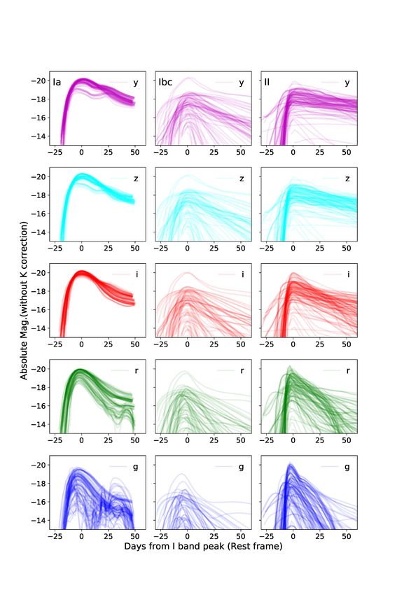
ity along the SN phase. Each time the number of input
epochs increases, the SN Ia probability, i.e., the output of
the classifier, is updated. In figure 15 (Upper panel), we
plotted the SN Ia probability at each epoch for each of 300
SNe labeled as Ia and non-Ia based on the SALT2 fitting.
The use of this result enabled us to measure the last epoch Fig. 15. Upper panel: Transition of Ia probability of SNe after first detection.
at which the correct type is classified, i.e., the epoch after Each line corresponds to one of the SNe. Different colors indicate different
which no further change in the classification occurs. The labels, with red being Ia and blue being non-Ia. Lower panel: Cumulative
ratio for the epoch at which SNe are finally correctly classified.
lower panel shows the cumulative ratio for the epoch. The
figure shows that the classification performance improves
with time and that 80% of supernovae are correctly clas-
sified approximately 30 days after their first detection. In
this figure, the initial cumulative ratio is lower than the
accuracy shown in figure 14 because certain SNe that are
initially correctly classified could ultimately be misclassi-
fied as a wrong type.
Figure 16 shows the transitions of SN Ia probability as
a function of the number of days from the peak for 26 SNe
selected as HST targets in the HSC survey, and the average
of these transitions. The SN Ia probability for the average
of the candidates is greater than 0.8 three weeks before the
peak. This means that our classifier accomplishes the task
described in subsection 2.1 by identifying good candidate
SNe even when it only has information acquired before the
SN peak.
6 Discussion
Fig. 16. Ia probability transitions of 26 HST targets. Each of the lighter lines
6.1 Factors affecting classifier performance represents the variation for individual HST targets, and the red line is the
average of these lines.
In this study, we applied our classifier to actual HSC survey
data to evaluate its classification performance. By classify-
ing actual data with our method, we determined that theYou can also read