Ensemble models from machine learning: an example of wave runup and coastal dune erosion - Nat ...
←
→
Page content transcription
If your browser does not render page correctly, please read the page content below
Nat. Hazards Earth Syst. Sci., 19, 2295–2309, 2019
https://doi.org/10.5194/nhess-19-2295-2019
© Author(s) 2019. This work is distributed under
the Creative Commons Attribution 4.0 License.

Ensemble models from machine learning: an example
of wave runup and coastal dune erosion
Tomas Beuzen1 , Evan B. Goldstein2 , and Kristen D. Splinter1
1 Water
      Research Laboratory, School of Civil and Environmental Engineering, UNSW Sydney, Sydney, NSW, Australia
2 Departmentof Geography, Environment, and Sustainability, University of North Carolina at Greensboro,
Greensboro, NC, USA

Correspondence: Tomas Beuzen (t.beuzen@unsw.edu.au)

Received: 14 March 2019 – Discussion started: 2 April 2019
Revised: 7 September 2019 – Accepted: 11 September 2019 – Published: 22 October 2019

Abstract. After decades of study and significant data col-       1   Introduction
lection of time-varying swash on sandy beaches, there is no
single deterministic prediction scheme for wave runup that       Wave runup is important for characterizing the vulnerability
eliminates prediction error – even bespoke, locally tuned pre-   of beach and dune systems and coastal infrastructure to wave
dictors present scatter when compared to observations. Scat-     action. Wave runup is typically defined as the time-varying
ter in runup prediction is meaningful and can be used to cre-    vertical elevation of wave action above ocean water levels
ate probabilistic predictions of runup for a given wave cli-     and is a combination of wave swash and wave setup (Hol-
mate and beach slope. This contribution demonstrates this        man, 1986; Stockdon et al., 2006). Most parameterizations
using a data-driven Gaussian process predictor; a probabilis-    of wave runup use deterministic equations that output a sin-
tic machine-learning technique. The runup predictor is devel-    gle value for either the maximum runup elevation in a given
oped using 1 year of hourly wave runup data (8328 observa-       time period, Rmax , or the elevation exceeded by 2 % of runup
tions) collected by a fixed lidar at Narrabeen Beach, Sydney,    events in a given time period, R2 , based on a given set of in-
Australia. The Gaussian process predictor accurately predicts    put conditions. In the majority of runup formulae, these input
hourly wave runup elevation when tested on unseen data with      conditions are easily obtainable parameters such as signifi-
a root-mean-squared error of 0.18 m and bias of 0.02 m. The      cant wave height, peak wave period, and beach slope (Atkin-
uncertainty estimates output from the probabilistic GP pre-      son et al., 2017; Holman, 1986; Hunt, 1959; Ruggiero et
dictor are then used practically in a deterministic numerical    al., 2001; Stockdon et al., 2006). However, wave dispersion
model of coastal dune erosion, which relies on a parame-         (Guza and Feddersen, 2012), wave spectrum (Van Oorschot
terization of wave runup, to generate ensemble predictions.      and d’Angremond, 1969), nearshore morphology (Cohn and
When applied to a dataset of dune erosion caused by a storm      Ruggiero, 2016), bore–bore interaction (García-Medina et
event that impacted Narrabeen Beach in 2011, the ensem-          al., 2017), tidal stage (Guedes et al., 2013), and a range
ble approach reproduced ∼ 85 % of the observed variability       of other possible processes have been shown to influence
in dune erosion along the 3.5 km beach and provided clear        swash zone processes. Since typical wave runup parameter-
uncertainty estimates around these predictions. This work        izations do not account for these more complex processes,
demonstrates how data-driven methods can be used with tra-       there is often significant scatter in runup predictions when
ditional deterministic models to develop ensemble predic-        compared to observations (e.g., Atkinson et al., 2017; Stock-
tions that provide more information and greater forecasting      don et al., 2006). Even flexible machine-learning approaches
skill when compared to a single model using a deterministic      based on extensive runup datasets or consensus-style “model
parameterization – an idea that could be applied more gener-     of models” do not resolve prediction scatter in runup datasets
ally to other numerical models of geomorphic systems.            (e.g., Atkinson et al., 2017; Passarella et al., 2018b; Power
                                                                 et al., 2019). This suggests that the development of a per-
                                                                 fect deterministic parameterization of wave runup, especially

Published by Copernicus Publications on behalf of the European Geosciences Union.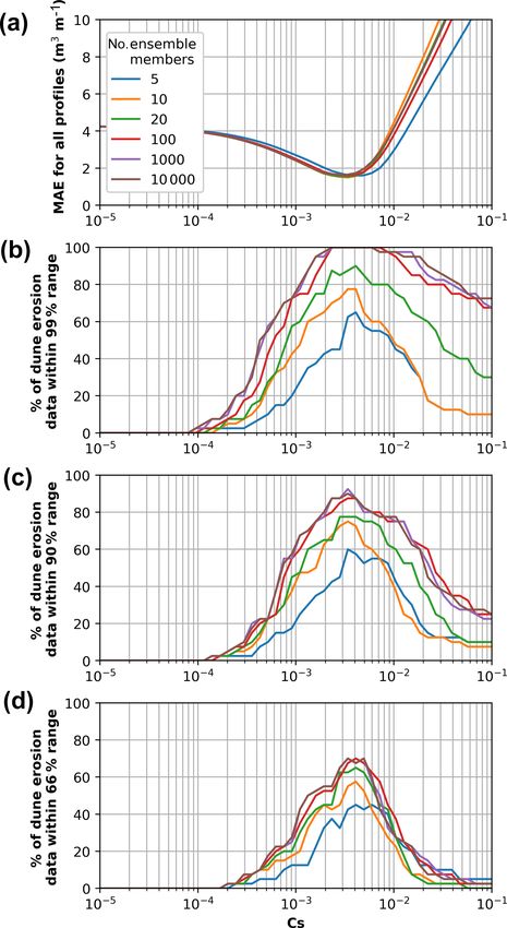
2296                                T. Beuzen et al.: Ensemble models from machine learning: an example of wave runup

with only reduced, easily obtainable inputs (i.e., wave height,   ically used Gaussian processes to model coastal processes
wave period, and beach slope), is improbable.                     such as large-scale coastline erosion (Kupilik et al., 2018)
   The resulting inadequacies of a single deterministic pa-       and estuarine hydrodynamics (Parker et al., 2019).
rameterization of wave runup can cascade up through the              The work presented here is focused on using a Gaussian
scales to cause error in any larger model that uses a runup       process to build a data-driven probabilistic predictor of wave
parameterization. It therefore makes sense to clearly incor-      runup that includes estimates of uncertainty. While quanti-
porate prediction uncertainty into wave runup predictions. In     fying uncertainty in runup predictions from data is useful in
disciplines such as hydrology and meteorology, with a more        itself, the benefit of this methodology is in explicitly includ-
established tradition of forecasting, model uncertainty is of-    ing the uncertainty with the runup predictor in a larger model
ten captured by using ensembles (e.g., Bauer et al., 2015;        that uses a runup parameterization, such as a coastal dune
Cloke and Pappenberger, 2009). The benefits of ensemble           erosion model. Dunes on sandy coastlines provide a natu-
modelling are typically superior skill and the explicit inclu-    ral barrier to storm erosion by absorbing the impact of inci-
sion of uncertainty in predictions by outputting a range of       dent waves and storm surge and helping to prevent or delay
possible model outcomes. Commonly used methods of gen-            flooding of coastal hinterland and infrastructure (Mull and
erating ensembles include combining different models (Lim-        Ruggiero, 2014; Sallenger, 2000; Stockdon et al., 2007). The
ber et al., 2018) or perturbing model parameters, initial con-    accurate prediction of coastal dune erosion is therefore crit-
ditions, and/or input data (e.g., via Monte Carlo simulations;    ical for characterizing the vulnerability of dune and beach
e.g., Callaghan et al., 2013).                                    systems and coastal infrastructure to storm events. A vari-
   An alternative approach to quantify prediction uncertainty     ety of methods are available for modelling dune erosion,
is to incorporate scatter about a mean prediction into model      including simple conceptual models relating hydrodynamic
parameterizations. For example, wave runup predictions at         forcing, antecedent morphology, and dune response (Sal-
every time step could be modelled with a deterministic pa-        lenger, 2000); empirical dune-impact models that relate time-
rameterization plus a noise component that captures the           dependent dune erosion to the force of wave impact at the
scatter about the deterministic prediction caused by unre-        dune (Erikson et al., 2007; Larson et al., 2004; Palmsten and
solved processes. If parameterizations are stochastic, or have    Holman, 2012); data-driven machine-learning models (Plant
a stochastic component, repeated model runs (given identical      and Stockdon, 2012); and more complex physics-based mod-
initial and forcing conditions) produce different model out-      els (Roelvink et al., 2009). In this study, we focus on dune-
puts – an ensemble – that represent a range of possible val-      impact models, which are simple, commonly used models
ues the process could take. This is broadly analogous to the      that typically rely on a parameterization of wave runup to
method of stochastic parameterization used in the weather         model time-dependent dune erosion. As inadequacies in the
forecasting community for sub-grid-scale processes and pa-        runup parameterization can jeopardize the success of model
rameterizations (Berner et al., 2017). In these applications,     results (Overbeck et al., 2017; Palmsten and Holman, 2012;
stochastic parameterization has been shown to produce bet-        Splinter et al., 2018), it makes sense to use a runup predictor
ter predictions than traditional ensemble methods and is now      that includes prediction uncertainty.
routinely used by many operational weather forecasting cen-          The overall aim of this work is to demonstrate how prob-
tres (Berner et al., 2017; Buchanan, 2018).                       abilistic data-driven methods can be used with deterministic
   Stochastically varying a deterministic wave runup param-       models to develop ensemble predictions, an idea that could
eterization to form an ensemble still requires defining the       be applied more generally to other numerical models of geo-
stochastic term – i.e., the stochastic element that should be     morphic systems. Section 2 first describes the Gaussian pro-
added to the predicted runup at each model time step. An al-      cess model theory. In Sect. 3 the Gaussian process runup pre-
ternative to specifying a predefined distribution or a noise      dictor is developed. In Sect. 4 an example application of the
term added to a parameterization is to learn and parame-          Gaussian process predictor of runup inside a morphodynamic
terize the variability in wave runup from observational data      model of coastal dune erosion to build a hybrid model (Gold-
using machine-learning techniques. Machine learning has           stein and Coco, 2015; Krasnopolsky and Fox-Rabinovitz,
had a wide range of applications in coastal morphodynam-          2006) that can generate ensemble output is presented. A dis-
ics research (Goldstein et al., 2019) and has shown specific      cussion of the results and technique is provided in Sect. 5
utility in understanding swash processes (Passarella et al.,      followed by conclusions in Sect. 6. The data and code used
2018b; Power et al., 2019) as well as storm-driven erosion        to develop the Gaussian process runup predictor in this paper
(Beuzen et al., 2017, 2018; den Heijer et al., 2012; Goldstein    are publicly available at https://github.com/TomasBeuzen/
and Moore, 2016; Palmsten et al., 2014; Plant and Stock-          BeuzenEtAl_2019_NHESS_GP_runup_model (Beuzen and
don, 2012). While many machine-learning algorithms and            Goldstein, 2019).
applications are often used to optimize deterministic predic-
tions, a Gaussian process is a probabilistic machine-learning
technique that directly captures model uncertainty from data
(Rasmussen and Williams, 2006). Recent work has specif-

Nat. Hazards Earth Syst. Sci., 19, 2295–2309, 2019                        www.nat-hazards-earth-syst-sci.net/19/2295/2019/
T. Beuzen et al.: Ensemble models from machine learning: an example of wave runup 2297
2 Gaussian processes location x, while the covariance function encodes the corre-
lation between the function values at locations in x.
2.1 Gaussian process theory These concepts of GP development are further described
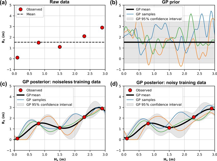
using a hypothetical dataset of significant wave height (Hs )
Gaussian processes (GPs) are data-driven, non-parametric versus wave runup (R2 ) shown in Fig. 1a. The first step of
models. A brief introduction to GPs is given here; for a more GP modelling is to constrain the infinite set of functions
detailed introduction the reader is referred to Rasmussen and that could fit a dataset by defining a prior distribution over
Williams (2006). There are two main approaches to deter- the space of functions. This prior distribution encodes be-
mine a function that best parameterizes a process over an in- lief about what the underlying function is expected to look
put space: (1) select a class of functions to consider, e.g., like (e.g., smooth/erratic, cyclic/random) before constrain-
polynomial functions, and best fit the functions to the data (a ing the model with any observed training data. Typically it
parametric approach); or (2) consider all possible functions is assumed that the mean function of the GP prior, m(x),
that could fit the data, and assign higher weight to functions is 0 everywhere, to simplify notation and computation of the
that are more likely (a non-parametric approach) (Rasmussen model (Rasmussen and Williams, 2006). Note that this does
and Williams, 2006). In the first approach it is necessary to not limit the GP posterior to be a constant mean process. The
decide on a class of functions to fit to the data – if all or parts covariance function, k(x, x 0 ), ultimately encodes what the
of the data are not well modelled by the selected functions, underlying functions look like because it controls how sim-
then the predictions may be poor. In the second approach ilar the function value at one input point is to the function
there is an infinite set of possible functions that could fit a value at other input points.
dataset (imagine the number of paths that could be drawn be- There are many different types of covariance functions or
tween two points on a graph). A GP addresses the problem kernels. One of the most common, and the one used in this
of infinite possible functions by specifying a probability dis- study, is the squared exponential covariance function:
tribution over the space of possible functions that fit a given "
D
#
dataset. Based on this distribution, the GP quantifies what 2
X 1 2
k xi , xj = σf exp − x − xd,j
2 d,i
, (2)
function most likely fits the underlying process generating d=1 2ld
the data and gives confidence intervals for this estimate. Ad-
where σf is the signal variance and l is known as the length
ditionally, random samples can also be drawn from the dis-
scale, both of which are hyperparameters in the model that
tribution to provide examples of what different functions that
can be estimated from data (discussed further in Sect. 2.2).
fit the dataset might look like.
Together the mean function and covariance function specify
A GP is defined as a collection of random variables, any
a multivariate Gaussian distribution:
finite set of which has a multivariate Gaussian distribution.
The random variables in a GP represent the value of the un- f (x) ∼ N (0, K), (3)
derlying function that describes the data, f (x), at location x. where f is the output of the prior distribution, the mean
The typical workflow for a GP is to define a prior distribution function is assumed to be 0, and K is the covariance matrix
over the space of possible functions that fit the data, form a made by evaluating the covariance function at arbitrary input
posterior distribution by conditioning the prior on observed points that lie within the domain being modelled (i.e., K(x,
input/output data pairs (“training data”), and to then use this x)i,j = k(xi , xj )). Random sample functions can be drawn
posterior distribution to predict unknown outputs at other in- from this prior distribution as demonstrated in Fig. 1b.
put values (“testing data”). The key to GP modelling is the The goal is to determine which of these functions actu-
use of the multivariate Gaussian distribution, which has sim- ally fit the observed data points (training data) in Fig. 1a.
ple closed form solutions to the aforementioned conditioning This can be achieved by forming a posterior distribution on
process, as described below. the function space by conditioning the prior with the train-
Whereas a univariate Gaussian distribution is defined by ing data. Roughly speaking, this operation is mathematically
a mean and variance (i.e., (µ, σ 2 )), a GP (a multivariate equivalent to drawing an infinite number of random func-
Gaussian distribution) is completely defined by a mean func- tions from the multivariate Gaussian prior (Eq. 3) and then
tion m(x) and covariance function k(x, x 0 ) (also known as a rejecting those that do not agree with the training data. As
“kernel”), and it is typically denoted as mentioned above, the multivariate Gaussian offers a simple,
closed form solution to this conditioning. Assuming that our
f (x) ∼ N (m(x), k(x, x 0 )), (1) observed training data are noiseless (i.e., y exactly represents
the value of the underlying function f ) then we can condition
where x is an input vector of dimension D (x ∈ R D ), and the prior distribution with the training data samples (x, y) to
f is the unknown function describing the data. Note that for define a posterior distribution of the function value (f ∗ ) at
the remainder of this paper, a variable denoted in bold text arbitrary test inputs (x ∗ ):
represents a vector. The mean function, m(x), describes the
expected mean value of the function describing the data at f ∗ |y ∼ N K∗ K−1 y, K∗∗ − K∗ K−1 KT∗ , (4)
www.nat-hazards-earth-syst-sci.net/19/2295/2019/ Nat. Hazards Earth Syst. Sci., 19, 2295–2309, 2019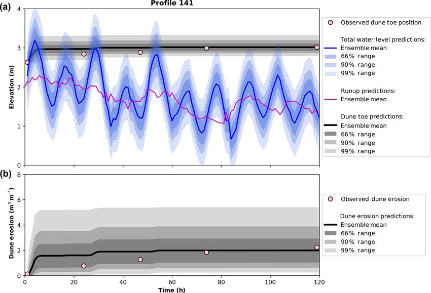
2298                                   T. Beuzen et al.: Ensemble models from machine learning: an example of wave runup

Figure 1. (a) Five hypothetical random observations of significant wave height (Hs ) and 2 % wave runup elevation (R2 ). (b) The Gaussian
process (GP) prior distribution. (c) The GP posterior distribution, formed by conditioning the prior distribution in (b) with the observed
data points in (a), assuming the observations are noise-free. (d) The GP posterior distribution conditioned on the observations with a noise
component.

where f ∗ is the output of the posterior distribution at the de-        where σn2 is the variance of the noise and δij is a Kronecker
sired test points x ∗ , y is the training data outputs at inputs x,     delta which is 1 if i = j and 0 otherwise. The squared expo-
K∗ is the covariance matrix made by evaluating the covari-              nential kernel and white noise kernel are closed under addi-
ance function (Eq. 2) between the test inputs x ∗ and training          tion and product (Rasmussen and Williams, 2006), such that
inputs x (i.e., k(x ∗ , x)), K is the covariance matrix made            they can simply be combined to form a custom kernel for use
by evaluating the covariance function between training data             in the GP:
points x, and K∗∗ is the covariance matrix made by evalu-                                    (
                                                                                                 D
                                                                                                                      )
                                                                                      2
                                                                                                X    1             2
                                                                                                                        + σn2 δij . (7)

ating the covariance function between test points x ∗ . Func-           k xi , xj = σf exp −             x − xd,j
                                                                                                    2l 2 d,i
tion values can be sampled from the posterior distribution as                                   d=1 d
shown in Fig. 1c. These samples represent random realiza-               The combination of kernels to model different signals
tions of what the underlying function describing the training           in a dataset (that vary over different spatial or temporal
data could look like.                                                   timescales) is common in applications of GPs (Rasmussen
   As stated earlier, in Eq. (4) and Fig. 1c there is an assump-        and Williams, 2006; Reggente et al., 2014; Roberts et al.,
tion that the training data are noiseless and represent the ex-         2013). Samples drawn from the resultant noisy posterior dis-
act value of the function at the specific point in input space.         tribution are shown in Fig. 1d, in which the GP can now be
In reality, there is error associated with observations of phys-        seen to not fit the observed training data precisely.
ical systems, such that
                                                                        2.2    Gaussian process kernel optimization
y = f (x) + ε,                                                 (5)
                                                                        In Eq. (7) there are three hyperparameters: the signal vari-
where ε is assumed to be independent identically distributed            ance (σf ), the length scale (l), and the noise variance (σn ).
Gaussian noise with variance σn2 . This noise can be incorpo-           These hyperparameters are typically unknown but can be es-
rated into the GP modelling framework through the use of a              timated and optimized based on the particular dataset. Here,
white noise kernel that adds an element of Gaussian white               this optimization is performed by using the typical method-
noise into the model:                                                   ology of maximizing the log marginal likelihood of the ob-
                                                                        served data y given the hyperparameters:
k xi , xj = σn2 δij ,

                                                               (6)      log p y|x, σf , l, σn .                                    (8)

Nat. Hazards Earth Syst. Sci., 19, 2295–2309, 2019                               www.nat-hazards-earth-syst-sci.net/19/2295/2019/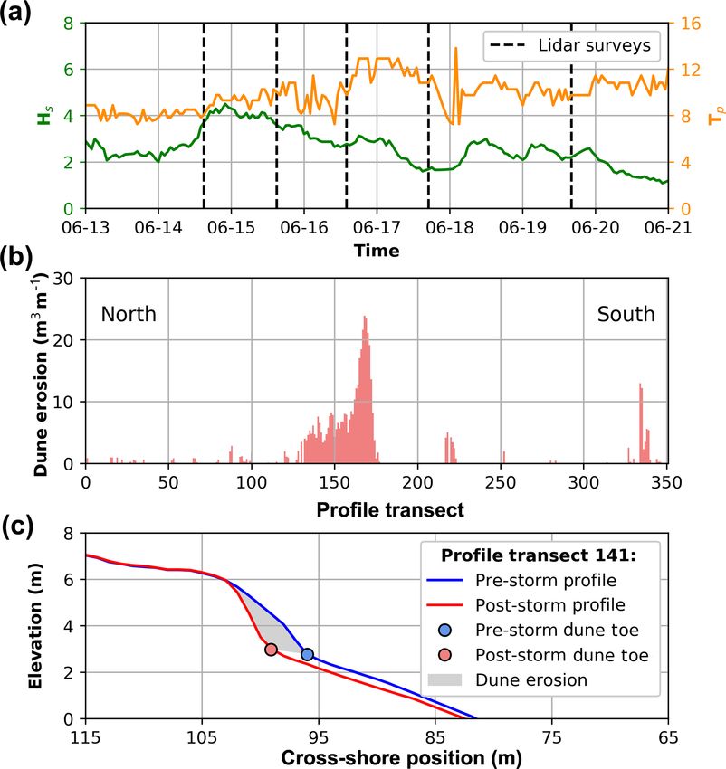
T. Beuzen et al.: Ensemble models from machine learning: an example of wave runup                                              2299

The Python toolkit scikit-learn (Pedregosa et al., 2011) was          and k-means clustering (Camus et al., 2011), the MDA rou-
used to develop the GP described in this study. For the Reader        tine used in this study was found in preliminary testing (not
unfamiliar with the Python programming language, alter-               presented) to produce the best GP performance with the least
native programs for developing Gaussian processes include             computational expense.
Matlab (Rasmussen and Nickisch, 2010) and R (Dancik and
Dorman, 2008; MacDonald et al., 2015).
                                                                      3     Development of a Gaussian process runup model
2.3   Training a Gaussian process model
                                                                      3.1    Runup data
It is standard practice in the development of data-driven
machine-learning models to divide the available dataset into          In 2014, an extended-range lidar (light detection and rang-
training, validation, and testing subsets. The training data are      ing) device (SICK LD-LRS 2110) was permanently installed
used to fit model parameters. The validation data are used to         on the rooftop of a beachside building (44 m a.m.s.l. – above
evaluate model performance, and the model hyperparameters             mean sea level) at Narrabeen–Collaroy Beach (hereafter re-
are usually varied until performance on the validation data is        ferred to simply as Narrabeen) on the southeast coast of
optimized. Once the model is optimized, the remaining test            Australia (Fig. 2). Since 2014, this lidar has continuously
dataset is used to objectively evaluate its performance and           scanned a single cross-shore profile transect extending from
generalizability. A decision must be made about how to split          the base of the beachside building to a range of 130 m, captur-
a dataset into training, validation, and testing subsets. There       ing the surface of the beach profile and incident wave swash
are many different approaches to handle this splitting pro-           at a frequency of 5 Hz in both daylight and non-daylight
cess; for example, random selection, cross validation, strat-         hours. Specific details of the lidar setup and functioning can
ified sampling, or a number of other deterministic sampling           be found in Phillips et al. (2019).
techniques (Camus et al., 2011). The exact technique used                Narrabeen Beach is a 3.6 km long embayed beach bounded
to generate the data subsets often depends on the problem at          by rocky headlands. It is composed of fine to medium quartz
hand. Here, there were two constraints to be considered: first,       sand (D50 ≈ 0.3 mm), with a ∼ 30 % carbonate fraction. Off-
the computational expense of GPs scales by O(n3 ) (Ras-               shore, the coastline has a steep and narrow (20–70 km) con-
mussen and Williams, 2006), so it is desirable to keep the            tinental shelf (Short and Trenaman, 1992). The region is mi-
training set as small as possible without deteriorating model         crotidal and semidiurnal with a mean spring tidal range of
performance; and, secondly, machine-learning models typi-             1.6 m and has a moderate to high energy deep water wave cli-
cally perform poorly with out-of-sample predictions (i.e., ex-        mate characterized by persistent long-period south-southeast
trapolation), so it is desirable to include in the training set the   swell waves that is interrupted by storm events (significant
data samples that capture the full range of variability in the        wave height > 3 m) typically 10–20 times per year (Short
data. Based on these constraints, we used a maximum dis-              and Trenaman, 1992). In the present study, approximately
similarity algorithm (MDA) to divide the available data into          1 year of the high-resolution wave runup lidar dataset avail-
training, validation, and testing sets.                               able at Narrabeen is used to develop a data-driven parame-
    The MDA is a deterministic routine that iteratively adds          terization of the 2 % exceedance of wave runup (R2 ). Data
a data point to the training set based on how dissimilar it           used to develop this parameterization were at hourly resolu-
is to the data already included in the training set. Camus et         tion and include R2 , the beach slope (β), offshore significant
al. (2011) provide a comprehensive introduction to the MDA            wave height (Hs ), and peak wave period (Tp ). These data are
selection routine, and it has been previously used in machine-        described below and have been commonly used to parame-
learning studies (e.g., Goldstein et al., 2013). Briefly, to ini-     terize R2 in other empirical models of wave runup (e.g., Hol-
tialize the MDA routine, the data point with the maximum              man, 1986; Hunt, 1959; Stockdon et al., 2006).
sum of dissimilarity (defined by Euclidean distance) to all              Individual wave runup elevation on the beach profile was
other data points is selected as the first data point to be added     extracted on a wave-by-wave basis from the lidar dataset
to the training dataset. Additional data points are included in       (Fig. 2c) using a neural network runup detection tool devel-
the training set through an iterative process whereby the next        oped by Simmons et al. (2019). Hourly R2 was calculated as
data point added is the one with maximum dissimilarity to             the 2 % exceedance value for a given hour of wave runup ob-
those already in the training set – this process continues un-        servations. β was calculated as the linear (best-fit) slope of
til a user-defined training set size is reached. In this way the      the beach profile over which 2 standard deviations of wave
MDA routine produces a set of training data that captures the         runup values were observed during the hour. Hourly Hs and
range of variability present in the full dataset. The data not        Tp data were obtained from the Sydney Waverider buoy, sit-
selected for the training set are equally and randomly split to       uated 11 km offshore of Narrabeen in ∼ 80 m water depth.
form the validation dataset and test dataset. While alternative       Narrabeen is an embayed beach, where prominent rocky
data-splitting routines are available, including simple random        headlands both attenuate and refract incident waves. To re-
sampling, stratified random sampling, self-organizing maps,           move these effects in the wave data and to emulate an open

www.nat-hazards-earth-syst-sci.net/19/2295/2019/                              Nat. Hazards Earth Syst. Sci., 19, 2295–2309, 2019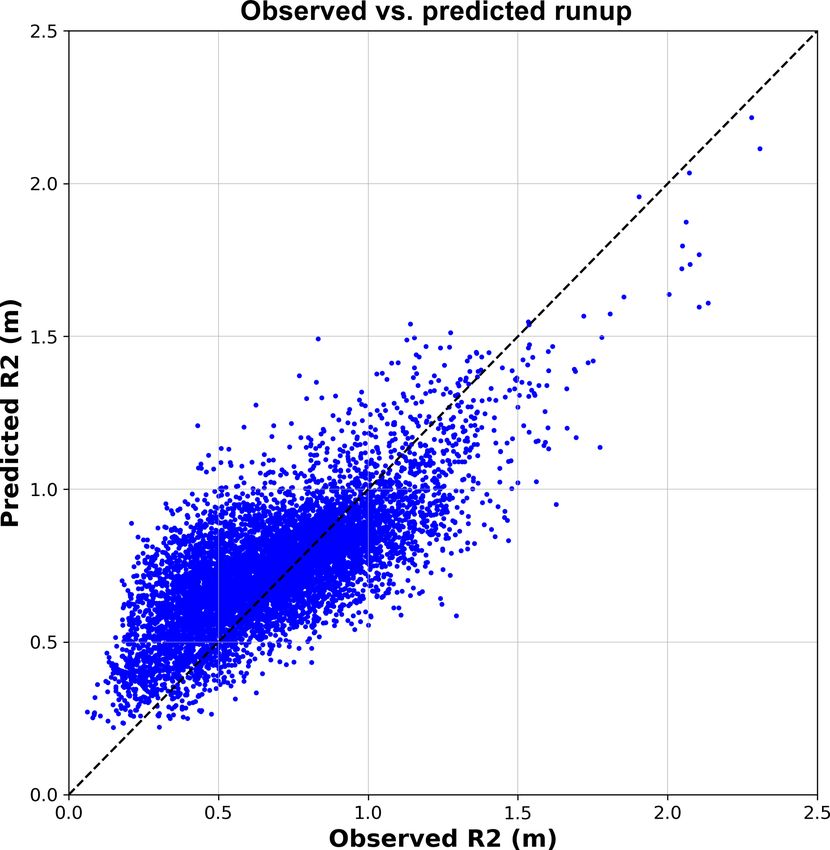
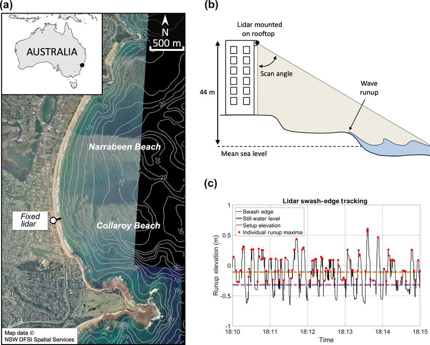
2300                                   T. Beuzen et al.: Ensemble models from machine learning: an example of wave runup

Figure 2. (a) Narrabeen Beach, located on the southeast coast of Australia. (b) Conceptual figure of the fixed lidar setup. (c) A 5 min extract
of runup elevation extracted from the lidar data; individual runup maxima are marked with red circles.

coastline and generalize the parameterization of R2 presented
in this study, offshore wave data were first transformed to
a nearshore equivalent (10 m water depth) using a precalcu-
lated lookup table generated with the SWAN spectral wave
model based on a 10 m resolution grid (Booij et al., 1999) and
then reverse shoaled back to deep water wave data. A total of
8328 hourly samples of R2 , β, Hs , and Tp were extracted to
develop a parameterization of R2 in this study. Histograms of
these data are shown in Fig. 3.

3.2    Training data for the GP runup predictor

To determine the optimum training set size, kernel, and
model hyperparameters, a number of different user-defined
training set sizes were trialled using the MDA selection rou-
tine discussed in Sect. 2.3. The GP was trained using dif-
ferent amounts of data and hyperparameters were optimized
on the validation dataset only. It was found that a training
set size of only 5 % of the available dataset (training dataset:
416 of 8328 available samples; validation dataset: 3956 sam-              Figure 3. Histograms of the 8328 data samples extracted from the
ples; testing dataset: 3956 samples) was required to develop              Narrabeen lidar: (a) significant wave height (Hs ); (b) peak wave
an optimum GP model. Training data sizes beyond this value                period (Tp ); (c) beach slope (β); and (d) 2 % wave runup eleva-
produced negligible changes in GP performance but consid-                 tion (R2 ).
erable increases in computational demand, similar to findings
of previous work (Goldstein and Coco, 2014; Tinoco et al.,
2015). Results presented below discuss the performance of

Nat. Hazards Earth Syst. Sci., 19, 2295–2309, 2019                                www.nat-hazards-earth-syst-sci.net/19/2295/2019/
T. Beuzen et al.: Ensemble models from machine learning: an example of wave runup                                            2301

                                                                  Figure 5. (a) Percent of observed runup values captured within
                                                                  the range of ensemble predictions made by randomly sampling dif-
                                                                  ferent runup values from the Gaussian process. Only 10 randomly
                                                                  drawn models can form an ensemble that captures 95 % of the scat-
                                                                  ter in observed R2 values. (b) An experiment showing how much
                                                                  arbitrary error would need to be added to the mean GP runup pre-
                                                                  diction in order to capture scatter in R2 observations. The mean
Figure 4. Observed 2 % wave runup (R2 ) versus the R2 pre-        GP prediction would have to vary by 51 % in order to capture 95 %
dicted by the Gaussian process model. The root-mean-squared er-   of scatter in R2 observations.
ror (RMSE) is 0.36 m, bias (B) is 0.02 m, and squared correla-
tion (r 2 ) is 0.54.
                                                                  scatter in R2 (Fig. 5a). This process of drawing random sam-
                                                                  ples from the GP was repeated 100 times with results show-
the GP on the testing dataset which was not used in GP train-     ing that the above is true for any 10 random samples, with
ing or validation.                                                an average capture percentage of 95.7 % and range of 94.9 %
                                                                  to 96.1 % for 10 samples across the 100 trials. As a point
3.3   Runup predictor results
                                                                  of contrast, Fig. 5b shows how much arbitrary error would
Results of the GP R2 predictor on the 3956 test samples are       need to be added to the mean R2 prediction to capture scat-
shown in Fig. 4. This figure plots the mean GP predictions        ter about the mean to emulate the uncertainty captured by
against corresponding observations of R2 . The mean GP pre-       the GP. It can be seen that the mean R2 prediction would
diction performs well on the test data, with a root-mean-         need to vary by ±51 % to capture 95 % of the scatter present
squared error (RMSE) of 0.18 m and bias (B) of 0.02 m.            in the runup data. This demonstrates how random models of
For comparison, the commonly used R2 parameterization of          runup drawn from the GP effectively capture uncertainty in
Stockdon et al. (2006) tested on the same data has a RMSE         R2 predictions. These randomly drawn R2 models can be
of 0.36 m and B of 0.21 m. Despite the relatively accurate        used within a larger dune-impact model to produce an en-
performance of the GP on this dataset, there remains signif-      semble of dune erosion predictions that includes uncertainty
icant scatter in the observed versus predicted R2 in Fig. 4.      in runup predictions, as demonstrated in Sect. 4.
This is consistent with recent work by Atkinson et al. (2017)
showing that commonly used predictors of R2 always result
                                                                  4     Application of a Gaussian process runup predictor in
in scatter.
                                                                        a coastal dune erosion model
   As discussed in Sect. 1 scatter in runup predictions is
likely a result of unresolved processes in the model such as      4.1    Dune erosion model
wave dispersion, wave spectrum, nearshore morphology, or
a range of other possible processes. Regardless of the ori-       We use the dune erosion model of Larson et al. (2004) as an
gin, here this scatter (uncertainty) is used to form ensemble     example of how the GP runup predictor can be used to create
predictions. The GP developed here not only gives a mean          an ensemble of dune erosion predictions, and we thus pro-
prediction as used in Fig. 4, but it specifies a multivariate     vide probabilistic outcomes with uncertainty bands needed
Gaussian distribution from which different random functions       in coastal management. The dune erosion model is subse-
that describe the data can be sampled. Random samples of          quently referred to as LEH04 and is defined as follows:
wave runup from the GP can capture uncertainty around the
mean runup prediction (as was demonstrated in the hypothet-                           2 t
                                                                  dV = 4Cs (R2 − zb )       ,                             (9)
ical example in Fig. 1d). To assess how well the GP model                                 T
captures uncertainty, random samples are successively drawn
from the GP, and the number of R2 measurements captured           where dV (m3 m−1 ) is the volumetric dune erosion per unit
with each new draw are determined. Only 10 random sam-            width alongshore for a given time step t, zb (m) is the time-
ples drawn from the GP are required to capture 95 % of the        varying dune toe elevation, T (s) is the wave period for that

www.nat-hazards-earth-syst-sci.net/19/2295/2019/                          Nat. Hazards Earth Syst. Sci., 19, 2295–2309, 2019
2302 T. Beuzen et al.: Ensemble models from machine learning: an example of wave runup
time step, R2 (m) is the 2 % runup exceedance for that time
step, and Cs is the transport coefficient. Note that the original
equation used a best-fit relationship to define the runup term,
R (see Eq. 36 in Larson et al., 2004), rather than R2 . Subse-
quent modifications of the LEH04 model have been made to
adjust the collision frequency (i.e. the t/T term; e.g., Palm-
sten and Holman, 2012, and Splinter and Palmsten, 2012);
however, we retain the model presented in Eq. (9) for the
purpose of providing a simple illustrative example. At each
time step, dune volume is eroded in bulk, and the dune toe
is adjusted along a predefined slope (defined here as the lin-
ear slope between the pre- and post-storm dune toe) so that
erosion causes the dune toe to increase in elevation and re-
cede landward. Dune erosion and dune toe recession only
occurs when wave runup (R2 ) exceeds the dune toe (i.e.,
R2 − zb > 0) and cannot progress vertically beyond the max-
imum runup elevation. When R2 does not exceed zb , dV = 0.
The GP R2 predictor described in Sect. 3 is used to stochasti-
cally parameterize wave runup in the LEH04 model and form
ensembles of dune erosion predictions. The model is applied
to new data not used to train the GP R2 predictor, using de-
tailed observations of dune erosion caused by a large coastal
storm event at Narrabeen Beach, southeast Australia in 2011. Figure 6. June 2011 storm data. (a) Offshore Hs and Tp with ver-
tical dashed lines indicating the time of the lidar surveys, (b) mea-
4.2 June 2011 storm data sured (pre- vs. post-storm) dune erosion volumes for the 351 profile
transects extracted from lidar data, and (c) example pre- (blue) and
post-storm (red) profile cross sections showing dune toes (coloured
In June 2011 a large coastal storm event impacted the south- circles) and dune erosion volume (grey shading).
east coast of Australia. This event resulted in variable along-
shore dune erosion at Narrabeen Beach, which was pre-
cisely captured by airborne lidar immediately pre-, during,
and post-storm by five surveys conducted approximately 24 h generate stochastic parameterizations and create probabilis-
apart. Cross-shore profiles were extracted from the lidar data tic model ensembles (Eq. 9).
at 10 m alongshore intervals as described in detail in Splin- For each of the 351 available profiles, the pre-, during,
ter et al. (2018), resulting in 351 individual profiles (Fig. 6). and post-storm dune toe positions were defined as the lo-
The June 2011 storm lasted 120 h. Hourly wave data were cal maxima of curvature of the beach profile following the
recorded by the Sydney Waverider buoy located in ∼ 80 m method of Stockdon et al. (2007). Dune erosion at each pro-
water depth directly to the southeast of Narrabeen Beach. file was then defined as the difference in subaerial beach vol-
As with the hourly wave data used to develop the GP model ume landward of the pre-storm dune toe, as shown in Fig. 6c.
of R2 (Sect. 3.1), hourly wave data for each of the 351 pro- Of the 351 profiles, only 117 had storm-driven dune ero-
files for the June 2011 storm were obtained by first trans- sion (Fig. 6b). For the example demonstration presented here,
forming offshore wave data to the nearshore equivalent at only profiles for which the post-storm dune toe elevation was
10 m water depth directly offshore of each profile using the at the same or higher elevation than the pre-storm dune toe
SWAN spectral wave model (Booij et al., 1999) and then are considered, which is a basic assumption of the LEH04
reverse shoaling back to equivalent deep water wave data, model. Of the 117 profiles with storm erosion, 40 profiles
to account for the effects of wave refraction and attenuation met these criteria. For each of these profiles, the linear slope
caused by the distinctly curved Narrabeen embayment. The between the pre- and post-storm dune toe was used to project
tidal range during the storm event was measured in situ at the dune erosion calculated using the LEH04 model.
the Fort Denison tide gauge (located within Sydney Harbour The LEH04 dune erosion model (Eq. 9) has a single tune-
approximately 16 km south of Narrabeen) as 1.58 m (mean able parameter, the transport coefficient Cs . There is ambi-
spring tidal range at Narrabeen is 1.6 m). As can be seen in guity in the literature regarding the value of Cs . Larson et
Fig. 6 the wave conditions for the June 2011 storm lie within al. (2004) developed an empirical equation to relate Cs to
the range of the training dataset used to develop the GP runup wave height (Hrms ) and grain size (D50 ) using experimen-
predictor. The hydrodynamic time series and airborne lidar tal data. Values ranged from 1 × 10⁻⁵ to 1 × 10⁻¹ , and Lar-
observations of dune change are used to demonstrate how the son et al. (2004) used 1.7 × 10⁻⁴ based on field data from
LEH04 model can be used with the GP predictor of runup to Birkemeier et al. (1988). Palmsten and Holman (2012) used
Nat. Hazards Earth Syst. Sci., 19, 2295–2309, 2019 www.nat-hazards-earth-syst-sci.net/19/2295/2019/T. Beuzen et al.: Ensemble models from machine learning: an example of wave runup 2303 LEH04 to model dune erosion observed in a large wave tically, the mean of the ensemble is plotted, along with inter- tank experiment conducted at the O. H. Hinsdale Wave Re- vals capturing 66 %, 90 %, and 99 % of the ensemble output. search Laboratory at Oregon State University. The model These intervals are consistent with those used in IPCC for was shown to accurately reproduce dune erosion when ap- climate change predictions (Mastrandrea et al., 2010), and, plied in hourly time steps using a Cs of 1.34 × 10⁻³ , based in the context of the model results presented here, they repre- on the empirical equation determined by Larson et al. (2004). sent varying levels of confidence in the model output. For ex- Mull and Ruggiero (2014) used values of 1.7 × 10⁻⁴ and ample, there is high confidence that the real dune erosion will 1.34 × 10⁻³ as lower and upper bounds of Cs to model dune fall within the 66 % ensemble prediction range. Figure 7b erosion caused by a large storm event on the Pacific North- shows the time-varying predicted distribution of dune ero- west Coast of the USA and the laboratory experiment used sion volumes from the 10 000 LEH04 runs. It can be seen by Palmsten and Holman (2012). For the dune erosion exper- that while the mean value of the ensemble predictions de- iment, the value of 1.7×10⁻⁴ was found to predict dune ero- viates slightly from the observed dune erosion, the observed sion volumes closest to the observed erosion when applied erosion is still captured well within the 66 % envelope of pre- in a single time step, with an optimum value of 2.98 × 10⁻⁴ . dictions. Splinter and Palmsten (2012) found a best-fit Cs of 4 × 10⁻⁵ Pre- and post-storm dune erosion results for the 40 profiles in an application to modelling dune erosion caused by a using 10 000 ensemble members and Cs of 1.5 × 10⁻³ are large storm event that occurred on the Gold Coast, Australia. shown in Fig. 8. The squared correlation (r 2 ) for the observed Ranasinghe et al. (2012) found a Cs value of 1.5 × 10⁻³ in and predicted dune erosion volumes is 0.85. Many of the pro- an application at Narrabeen Beach, Australia. It is noted that files experienced only minor dune erosion (< 2.5 m3 m−1 ) Cs values in these studies are influenced by the time step and can be seen to be well predicted by the mean of the en- used in the model and the exact definition of wave runup, R, semble predictions. In contrast, the ensemble mean can be used (Larson et al., 2004; Mull and Ruggiero, 2014; Palmsten seen to under-predict dune erosion at profiles where high ero- and Holman, 2012; Splinter and Palmsten, 2012). In practice, sion volumes were observed (profiles 29–34 in Fig. 8), with Cs could be optimized to fit any particular dataset. However, some profiles not even captured by the uncertainty of the en- for predictive applications the optimum Cs value may not be semble. However, the ensemble range of predictions for these known in advance, since it is unclear if subsequent storms at particular profiles also has a large spread, indicative of high a given location will be well predicted using previously op- uncertainty in predictions and the potential for high erosion timized Cs values. A key goal of this work is to determine to occur. It should be noted that the results presented in Fig. 8 if using stochastic parameterizations to generate ensembles are based on an assumed (i.e., non-optimized) Cs value of that predict a range of dune erosion (based on uncertainty in 1.5 × 10⁻³ . Better prediction of large erosion events could the runup parameterization) can still capture observed dune potentially be achieved by increasing Cs or giving greater erosion even if the optimum Cs value is not known in ad- weighting to these events during calibration, but at the cost of vance. As such, a Cs value of 1.5×10⁻³ is used in this exam- over-predicting the smaller events. The exact effect of vary- ple application based on previous work at Narrabeen Beach ing Cs is quantified in Sect. 4.3. Importantly, Fig. 8 demon- by Ranasinghe et al. (2012). Sensitivity of model results to strates that, even with a non-optimized Cs , uncertainty in the the choice of Cs is further discussed in Sect. 4.3. GP predictions can provide useful information about the po- An example at a single profile (profile 141, located approx- tential for dune erosion, even if the mean dune erosion pre- imately half-way up the Narrabeen embayment as shown in diction deviates from the observation – a key advantage of Fig. 6b) of time-varying ensemble dune erosion predictions the GP approach over a deterministic approach. is provided in Fig. 7. It was previously shown in Fig. 5 that only 10 random samples drawn from the GP R2 predictor 4.3 The effect of Cs and ensemble size on dune erosion were required to capture 95 % of the scatter in the R2 data used to develop and test the GP. However, it is trivial to In Sect. 4.2, the application of the GP runup predictor within draw many more samples than this from the GP – for ex- the LEH04 model to produce an ensemble of dune erosion ample, drawing 10 000 samples takes less than 1 s on a stan- predictions was based on 10 000 ensemble members and a dard desktop computer. Therefore, to explore a large range Cs value of 1.5 × 10⁻³ . The sensitivity of results to the num- of possible runup scenarios during the 120 h storm event, ber of members in the ensemble and the value of the tunable 10 000 different runup time series are drawn from the GP parameter Cs in Eq. (9) is presented in Fig. 9. The mean ab- and used to run LEH04 at hourly intervals, thus producing solute error (MAE) between the mean ensemble dune erosion 10 000 model results of dune erosion. The effect of using predictions and the observed dune erosion, averaged across different ensemble sizes is explored in Sect. 4.3. Figure 7a all 40 profiles, varies for R2 ensembles of 5, 10, 20, 100, shows the time-varying distribution of the runup models 1000, and 10 000 members and Cs values ranging from 10−5 (blue) used to force LEH04 along with the time-varying pre- to 10−1 (Fig. 9). As can be seen in Fig. 9a and summarized diction distribution of dune toe elevations (grey) throughout in Table 1, the lowest MAE for the differing ensemble sizes the 120 h storm event. To interpret model output probabilis- is similar, ranging from 1.50 to 1.64 m3 m−1 , suggesting that www.nat-hazards-earth-syst-sci.net/19/2295/2019/ Nat. Hazards Earth Syst. Sci., 19, 2295–2309, 2019
2304 T. Beuzen et al.: Ensemble models from machine learning: an example of wave runup
Figure 7. Example of LEH04 used with the Gaussian process R2 predictor to form an ensemble of dune erosion predictions. A total of
10 000 runup models are drawn from the Gaussian process and used to force the LEH04 model. (a) Total water level (measured water
level + R2 ; blue) and dune toe elevation (grey) for the 120 h storm event. The bold coloured line is the mean of the ensemble, and shaded
areas represent the regions captured by 66 %, 90 %, and 99 % of the ensemble predictions. An example of just the R2 prediction (no measured
water level) from the Gaussian process is shown in the magenta line. Pink dots denote the observed dune toe elevation throughout the storm
event. (b) The corresponding ensemble of dune erosion predictions.
the value of 1.5 × 10⁻³ previously reported by Ranasinghe
et al. (2012) for Narrabeen Beach and within the range of
Cs values presented in Larson et al. (2004).
The key utility to using a data-driven GP predictor to pro-
duce ensembles is that a range of predictions at every lo-
cation is provided as opposed to a single erosion volume.
The ensemble range provides an indication of uncertainty in
predictions, which can be highly useful for coastal engineers
and managers taking a risk-based approach to coastal hazard
management. Figure 9b–d displays the percentage of dune
erosion observations from the 40 profiles captured within en-
semble predictions for Cs values ranging from 10−5 to 10−1 .
It can be seen that a high proportion of dune erosion obser-
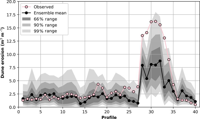
Figure 8. Observed (pink dots) and predicted (black dots) dune ero- vations are captured within the 66 %, 90 %, and 99 % ensem-
sion volumes for the 40 modelled profiles, using 10 000 runup mod-
ble envelope across several orders of magnitude Cs . While
els drawn from the Gaussian process and used to force the LEH04
the main purpose of using ensemble runup predictions within
model. Note that the 40 profiles shown are not uniformly spaced
along the 3.5 km Narrabeen embayment. The black dots represent LEH04 is to incorporate uncertainty in the runup prediction,
the ensemble mean prediction for each profile, while the shaded ar- this result demonstrates that the ensemble approach is less
eas represent the regions captured by 66 %, 90 %, and 99 % of the sensitive to the choice of Cs than a deterministic model and
ensemble predictions. so can be useful for forecasting with non-optimized model
parameters.
Results in Fig. 9 and Table 1 demonstrate that there is rela-
the number of ensemble members does not have a significant tively little difference in model performance when more than
impact on the resultant mean prediction. The lowest MAE 10 to 100 ensemble members are used, which is consistent
for the different ensemble sizes corresponds to Cs values be- with results presented previously in Fig. 5 that showed that
tween 2.8×10⁻³ (10 000 ensemble members) and 4.1×10⁻³ only 10 random samples drawn from the GP R2 predictor
(5 ensemble members), which is reasonably consistent with were required to capture 95 % of the scatter in the R2 data
Nat. Hazards Earth Syst. Sci., 19, 2295–2309, 2019 www.nat-hazards-earth-syst-sci.net/19/2295/2019/T. Beuzen et al.: Ensemble models from machine learning: an example of wave runup 2305
5 Discussion
5.1 Runup predictors
Studies of commonly used deterministic runup parameteriza-
tions such as those proposed by Hunt (1959), Holman (1986),
and Stockdon et al. (2006), amongst others, show that these
parameterizations are not universally applicable and there
remains no perfect predictor of wave runup on beaches
(Atkinson et al., 2017; Passarella et al., 2018a; Power et al.,
2019). This suggests that the available parameterizations do
not fully capture all the relevant processes controlling wave
runup on beaches (Power et al., 2019). Recent work has
used ensemble and data-driven methods to account for unre-
solved factors and complexity in runup processes. For exam-
ple, Atkinson et al. (2017) developed a model of models by
fitting a least-squares line to the predictions of several runup
parameterizations. Power et al. (2019) used a data-driven, de-
terministic, gene-expression programming model to predict
wave runup against a large dataset of runup observations.
Both of these approaches led to improved predictions, when
compared to conventional runup parameterizations, of wave
runup on the datasets tested in these studies.
The work presented in this study used a data-driven Gaus-
sian process (GP) approach to develop a probabilistic runup
predictor. While the mean predictions from the GP predic-
tor developed in this study using high-resolution lidar data
of wave runup were accurate (RMSE = 0.18 m) and better
than those provided by the Stockdon et al. (2006) formula
tested on the same data (RMSE = 0.36 m), the key advan-
tage of the GP approach over deterministic approaches is
that probabilistic predictions are output that is specifically
derived from data and implicitly accounts for unresolved pro-
cesses and uncertainty in runup predictions. Previous work
has similarly used GPs for efficiently and accurately quan-
tifying uncertainty in other environmental applications (e.g.,
Holman et al., 2014; Kupilik et al., 2018; Reggente et al.,
Figure 9. Results of the stochastic parameterization methodology 2014). While alternative approaches are available for gener-
for R2 ensembles of 5, 10, 20, 100, 1000, and 10 000 members and ating probabilistic predictions, such as Monte Carlo simula-
Cs values ranging from 10−5 to 10−1 . (a) The mean absolute er- tions (e.g., Callaghan et al., 2013), the GP approach offers a
ror (MAE) between the median ensemble dune erosion predictions method of deriving uncertainty explicitly from data, requires
and the observed dune erosion averaged across all 40 profiles. (b– no deterministic equations, and is computationally efficient
d) show the percentage of dune erosion observations that fall within (i.e., as discussed in Sect. 4.3, drawing 10 000 samples of
the 99 %, 90 %, and 66 % ensemble prediction ranges respectively. 120 h runup time series on a standard desktop computer took
less than 1 s). However, as discussed in Sect. 2.3, when devel-
oping a GP, or any machine-learning model, the training data
used to develop and test the GP. This suggests that the GP should include the full range of possible variability in the
approach efficiently captures scatter (uncertainty) in runup data to be modelled in order to avoid extrapolation. A limita-
predictions and subsequently dune erosion predictions, re- tion of using this data-driven approach for runup prediction
quiring on the order of 10 samples, which is significantly less is that it can be difficult to acquire a training dataset that cap-
than the 103 –106 runs typically used in Monte Carlo simula- tures all possible variability in the system from, for example,
tions to develop probabilistic predictions (e.g., Callaghan et longer-term trends in the wave climate, extreme events, or a
al., 2008; Li et al., 2013; Ranasinghe et al., 2012). potentially changing wave climate in the future (Semedo et
al., 2012).
www.nat-hazards-earth-syst-sci.net/19/2295/2019/ Nat. Hazards Earth Syst. Sci., 19, 2295–2309, 20192306 T. Beuzen et al.: Ensemble models from machine learning: an example of wave runup
Table 1. Quantitative summary of Fig. 9, showing the optimum Cs value for differing ensemble sizes, along with the associated mean absolute
error (MAE) and percent of the 40 dune erosion observations captured by the 66 %, 90 %, and 99 % ensemble prediction range.
Ensemble Optimum MAE r2 Percent Percent Percent
members Cs (m3 m−1 ) captured captured captured
in the 66 % in the 90 % in the 99 %
ensemble ensemble ensemble
range (%) range (%) range (%)
5 4.1 × 10⁻³ 1.59 0.86 45 57 65
10 3.4 × 10⁻³ 1.50 0.87 55 75 78
20 3.4 × 10⁻³ 1.54 0.86 62 78 88
100 3.3 × 10⁻³ 1.61 0.86 68 88 100
1000 2.8 × 10⁻³ 1.64 0.86 65 88 100
10 000 2.8 × 10⁻³ 1.64 0.86 65 88 100
5.2 Including uncertainty in dune erosion models ble 1, the simple LEH04 model (Eq. 9) applied here using the
GP runup predictor to generate ensemble prediction repro-
duced ∼ 85 % (based on the ensemble mean) of the observed
Uncertainty in wave runup predictions within dune-impact variability in dune erosion for the 40 profiles. While there
models can result in significantly varied predictions of dune are some discrepancies in the two modelling approaches, the
erosion. For example, the model of Larson et al. (2004) used ensemble approach clearly has an appreciable increase in
in this study only predicts dune erosion if runup elevation skill over the deterministic approach – attributed here to us-
exceeds the dune toe elevation and predicts a non-linear re- ing a runup predictor trained on local runup data – and the
lationship between runup that exceeds the dune toe and re- ensemble modelling approach. However, a major advantage
sultant dune erosion. Hence, if wave runup predictions are of the ensemble approach over the deterministic approach is
biased too low then no dune erosion will be predicted, and the provision of prediction uncertainty (e.g., Fig. 8). While
if wave runup is predicted too high then dune erosion may the mean ensemble prediction is not 100 % accurate, Table 1
be significantly over predicted. Ensemble modelling has be- shows that using just 100 samples can capture all the ob-
come standard practice in many areas of weather and cli- served variability in dune erosion within the ensemble out-
mate modelling (Bauer et al., 2015), as well as hydrologi- put.
cal modelling (Cloke and Pappenberger, 2009), and more re- The GP approach is a novel approach to building model
cently has been applied to coastal problems such as the pre- ensembles to capture uncertainty. Previous work modelling
diction of cliff retreat (Limber et al., 2018) as a method of beach and dune erosion has successfully used Monte Carlo
handling prediction uncertainty. While using a single deter- methods, which randomly vary model inputs within many
ministic model is computationally simple and provides one thousands of model iterations, to produce ensembles and
solution for a given set of input conditions, model ensembles probabilistic erosion predictions (e.g., Callaghan et al., 2008;
provide a range of predictions that can better capture the vari- Li et al., 2013; Ranasinghe et al., 2012). As discussed ear-
ety of mechanisms and stochasticity within a coastal system. lier in Sect. 4.3, the GP approach differs from Monte Carlo
The result is typically improved skill over deterministic mod- in that it explicitly quantifies uncertainty directly from data,
els (Atkinson et al., 2017; Limber et al., 2018) and a natural does not use deterministic equations, and can be computa-
method of providing uncertainty with predictions. tionally efficient.
As a quantitative comparison, Splinter et al. (2018) ap-
plied a modified version of the LEH04 model to the same
June 2011 storm dataset used in the work presented here with 6 Conclusion
a modified expression for the collision frequency (i.e. the
t/T term in Eq. 9) based on work by Palmsten and Hol- For coastal managers, the accurate prediction of wave runup
man (2012). The parameterization of Stockdon et al. (2006) as well as dune erosion is critical for characterizing the vul-
was used to estimate R2 in the model. The model was forced nerability of coastlines to wave-induced flooding, erosion of
hourly over the course of the storm, updating the dune toe, dune systems, and wave impacts on adjacent coastal infras-
recession slope, and profiles based on each daily lidar sur- tructure. While many formulations for wave runup have been
vey. Based on only the 40 profiles used in the present study, proposed over the years, none have proven to accurately pre-
results from Splinter et al. (2018) showed that the deter- dict runup over a wide range of conditions and sites of in-
ministic LEH04 approach reproduced 68 % (r 2 = 0.68) of terest. In this contribution, a Gaussian process (GP) with
the observed variability in dune erosion. As shown in Ta- over 8000 high-resolution lidar-derived wave runup obser-
Nat. Hazards Earth Syst. Sci., 19, 2295–2309, 2019 www.nat-hazards-earth-syst-sci.net/19/2295/2019/T. Beuzen et al.: Ensemble models from machine learning: an example of wave runup 2307
vations was used to develop a probabilistic parameterization Special issue statement. This article is part of the special issue “Ad-
of wave runup that quantifies uncertainty in runup predic- vances in computational modelling of natural hazards and geohaz-
tions. The mean GP prediction performed well on unseen ards”.
data, with a RMSE of 0.18 m, which is a significant improve-
ment over the commonly used R2 parameterization of Stock-
don et al. (2006) (RMSE of 0.36 m) used on the same data. Acknowledgements. Wave and tide data were kindly provided by
Further, only 10 randomly drawn models from the probabilis- the Manly Hydraulics Laboratory under the NSW Coastal Data Net-
work Program managed by OEH. The lead author is funded under
tic GP distribution were needed to form an ensemble that
the Australian Postgraduate Research Training Program.
captured 95 % of the scatter in the test data.
Coastal dune-impact models offer a method of predicting
dune erosion deterministically. As an example application of Financial support. This research has been supported by the Aus-
how the GP runup predictor can be used in geomorphic sys- tralian Research Council (grant nos. LP04555157, LP100200348,
tems, the uncertainty in the runup parameterization was prop- and DP150101339), the NSW Environmental Trust Environmental
agated through a deterministic dune erosion model to gener- Research Program (grant no. RD 2015/0128), and the DOD DARPA
ate ensemble model predictions and provide prediction un- (grant no. R0011836623/HR001118200064).
certainty. The hybrid dune erosion model performed well on
the test data, with a squared correlation (r 2 ) between the ob-
served and predicted dune erosion volumes of 0.85. Impor- Review statement. This paper was edited by Randall LeVeque and
tantly, the probabilistic output provided uncertainty bands of reviewed by two anonymous referees.
the expected erosion volumes, which is a key advantage over
deterministic approaches. Compared to traditional methods
of producing probabilistic predictions such as Monte Carlo, References
the GP approach has the advantage of learning uncertainty di-
rectly from observed data, it requires no deterministic equa- Atkinson, A. L., Power, H. E., Moura, T., Hammond, T., Callaghan,
tions, and is computationally efficient. D. P., and Baldock, T. E.: Assessment of runup predictions by
This work is an example of how a machine-learning model empirical models on non-truncated beaches on the south-east
Australian coast, Coast. Eng., 119, 15–31, 2017.
such as a GP can profitably be integrated into coastal mor-
Bauer, P., Thorpe, A., and Brunet, G.: The quiet revolution of nu-
phodynamic models (Goldstein and Coco, 2015) to provide
merical weather prediction, Nature, 525, 47–55, 2015.
probabilistic predictions for nonlinear, multidimensional Berner, J., Achatz, U., Batté, L., Bengtsson, L., Cámara, A. D. L.,
processes, and drive ensemble forecasts. Approaches com- Christensen, H. M., Colangeli, M., Coleman, D. R., Crommelin,
bining machine-learning methods with traditional coastal D., Dolaptchiev, S. I., and Franzke, C. L.: Stochastic parameter-
science and management models present a promising area ization: Toward a new view of weather and climate models, B.
for furthering coastal morphodynamic research. Future work Am. Meteorol. Soc., 98, 565–588, 2017.
is focused on using more data and additional inputs, such as Beuzen, T. and Goldstein, E. B.: Tomas-
offshore bar morphology and wave spectra, to improve the Beuzen/BeuzenEtAl_2019_NHESS_GP_runup_model:
GP runup predictor developed here, testing it at different lo- First release of repo (Version 0.1), Zenodo,
cations and integrating it into a real-time coastal erosion fore- https://doi.org/10.5281/zenodo.3401739, 2019.
Beuzen, T., Splinter, K. D., Turner, I. L., Harley, M. D., and
casting system.
Marshall, L.: Predicting storm erosion on sandy coastlines
using a Bayesian network, in: Proceedings of Australasian
Coasts & Ports: Working with Nature, 21–23 June 2017, Cairns,
Code and data availability. The data and code used to develop the Australia, 102–108, 2017.
Gaussian process runup predictor in this paper are publicly available Beuzen, T., Splinter, K., Marshall, L., Turner, I., Harley, M., and
at https://doi.org/10.5281/zenodo.3401739 (Beuzen and Goldstein, Palmsten, M.: Bayesian Networks in coastal engineering: Dis-
2019). tinguishing descriptive and predictive applications, Coast. Eng.,
135, 16–30, 2018.
Birkemeier, W. A., Savage, R. J., and Leffler, M. W.: A collection
Author contributions. The order of the authors’ names reflects the of storm erosion field data, Coastal Engineering Research Center,
size of their contribution to the writing of this paper. Vicksburg, MS, 1988.
Booij, N., Ris, R. C., and Holthuijsen, L. H.: A third-
generation wave model for coastal regions: 1. Model descrip-
Competing interests. The authors declare that they have no conflict tion and validation, J. Geophys. Res.-Oceans, 104, 7649–7666,
of interest. https://doi.org/10.1029/98jc02622, 1999.
Buchanan, M.: Ignorance as strength, Nat. Phys., 14, 428,
https://doi.org/10.1038/s41567-018-0133-9, 2018.
Callaghan, D. P., Nielsen, P., Short, A., and Ranas-
inghe, R.: Statistical simulation of wave climate and
www.nat-hazards-earth-syst-sci.net/19/2295/2019/ Nat. Hazards Earth Syst. Sci., 19, 2295–2309, 2019You can also read