Predicting Football Results Using Machine Learning Techniques
←
→
Page content transcription
If your browser does not render page correctly, please read the page content below

I NDIVIDUAL P ROJECT R EPORT

                    D EPARTMENT         OF   C OMPUTING
    I MPERIAL C OLLEGE OF S CIENCE , T ECHNOLOGY AND M EDICINE

    Predicting Football Results Using
     Machine Learning Techniques

                                                          Supervisor:
      Author:
                                                        Dr. Jonathan
      Corentin HERBINET
                                                PASSERAT-PALMBACH

                                June 20, 2018

Submitted in partial fulfillment of the requirements for the Joint Mathematics and
                  Computing MEng of Imperial College London
Abstract
Many techniques to predict the outcome of professional football matches have tra-
ditionally used the number of goals scored by each team as a base measure for eval-
uating a team’s performance and estimating future results. However, the number of
goals scored during a match possesses an important random element which leads to
large inconsistencies in many games between a team’s performance and number of
goals scored or conceded.

The main objective of this project is to explore different Machine Learning techniques
to predict the score and outcome of football matches, using in-game match events
rather than the number of goals scored by each team. We will explore different
model design hypotheses and assess our models’ performance against benchmark
techniques.

In this project, we developed an ’expected goals’ metric which helps us evaluate a
team’s performance, instead of using the actual number of goals scored. We com-
bined this metric with a calculation of a team’s offensive and defensive ratings which
are updated after each game and used to build a classification model predicting the
outcome of future matches, as well as a regression model predicting the score of
future games. Our models’ performance compare favourably to existing traditional
techniques and achieve a similar accuracy to bookmakers’ models.

i
Acknowledgments
Firstly, I would like to thank my supervisor, Dr. Jonathan Passerat-Palmbach, for his
constant support and help throughout the duration of the project. His confidence in
my work encouraged me to do my best.

Secondly, I would like to thank my second marker, Prof. William Knottenbelt, for
his expertise and for taking the time to discuss my ideas and to give me interesting
insight.

Finally, I would also like to thank my family, for always believing in me, my friends,
for their fun and support, Paul Vidal, for your friendship throughout our JMC adven-
ture, and Astrid Duval, for being there when I needed it the most.

iii
Contents

1 Introduction                                                                                                                          1
  1.1 Data Science for Football     .   .   .   .   .   .   .   .   .   .   .   .   .   .   .   .   .   .   .   .   .   .   .   .   .   1
  1.2 Motivation . . . . . . . .    .   .   .   .   .   .   .   .   .   .   .   .   .   .   .   .   .   .   .   .   .   .   .   .   .   2
  1.3 Objectives . . . . . . . .    .   .   .   .   .   .   .   .   .   .   .   .   .   .   .   .   .   .   .   .   .   .   .   .   .   3
  1.4 Challenges . . . . . . . .    .   .   .   .   .   .   .   .   .   .   .   .   .   .   .   .   .   .   .   .   .   .   .   .   .   5
  1.5 Contributions . . . . . .     .   .   .   .   .   .   .   .   .   .   .   .   .   .   .   .   .   .   .   .   .   .   .   .   .   5

2 Background                                                                                                                             6
  2.1 Football Rules & Events . . . . . . .                     .   .   .   .   .   .   .   .   .   .   .   .   .   .   .   .   .   .    6
  2.2 Machine Learning Techniques . . . .                       .   .   .   .   .   .   .   .   .   .   .   .   .   .   .   .   .   .    7
      2.2.1 Generalized Linear Models . .                       .   .   .   .   .   .   .   .   .   .   .   .   .   .   .   .   .   .    8
      2.2.2 Decision Trees . . . . . . . .                      .   .   .   .   .   .   .   .   .   .   .   .   .   .   .   .   .   .   10
      2.2.3 Probabilistic classification . .                    .   .   .   .   .   .   .   .   .   .   .   .   .   .   .   .   .   .   11
      2.2.4 Lazy learning . . . . . . . . .                     .   .   .   .   .   .   .   .   .   .   .   .   .   .   .   .   .   .   13
      2.2.5 Support Vector Machines . . .                       .   .   .   .   .   .   .   .   .   .   .   .   .   .   .   .   .   .   14
      2.2.6 Neural Network models . . .                         .   .   .   .   .   .   .   .   .   .   .   .   .   .   .   .   .   .   15
  2.3 Past Research . . . . . . . . . . . . .                   .   .   .   .   .   .   .   .   .   .   .   .   .   .   .   .   .   .   16
      2.3.1 Football prediction landscape                       .   .   .   .   .   .   .   .   .   .   .   .   .   .   .   .   .   .   16
      2.3.2 ELO ratings . . . . . . . . . .                     .   .   .   .   .   .   .   .   .   .   .   .   .   .   .   .   .   .   20
      2.3.3 Expected goals (xG) models .                        .   .   .   .   .   .   .   .   .   .   .   .   .   .   .   .   .   .   21

3 Dataset                                                                                                                               23
  3.1 Data origin . . . . . . . . . . . . . . . . . . . . . . . . . . . . . . . .                                                       23
  3.2 Data pre-processing . . . . . . . . . . . . . . . . . . . . . . . . . . . .                                                       24
  3.3 Data features . . . . . . . . . . . . . . . . . . . . . . . . . . . . . . .                                                       25

4 Design                                                                                                                                28
  4.1 Model components . . . . . . . . . . . . . . . . . . . . . . . . . . . .                                                          28
  4.2 Model choices . . . . . . . . . . . . . . . . . . . . . . . . . . . . . . .                                                       29

5 Implementation                                                                                                                        35
  5.1 General pipeline . . . . . . . . . . . . . . . . . . . . . . . . . . . . .                                                        35
  5.2 Luigi . . . . . . . . . . . . . . . . . . . . . . . . . . . . . . . . . . . .                                                     36

                                                    v
CONTENTS Table of Contents
6 Experimentation & Optimisation 39
6.1 Testing . . . . . . . . . . . . . . . . . . . . . . . . . . . . . . . . . . . 39
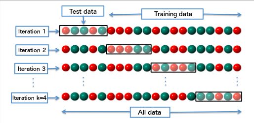
6.1.1 Cross-validation testing . . . . . . . . . . . . . . . . . . . . . 39
6.1.2 Testing metrics . . . . . . . . . . . . . . . . . . . . . . . . . . 39
6.2 Choice of models . . . . . . . . . . . . . . . . . . . . . . . . . . . . . 42
6.3 Parameter optimisation . . . . . . . . . . . . . . . . . . . . . . . . . . 45
6.3.1 OpenMOLE parameter optimisation . . . . . . . . . . . . . . . 45
6.3.2 Results . . . . . . . . . . . . . . . . . . . . . . . . . . . . . . . 46
6.3.3 Analysis of optimal parameters . . . . . . . . . . . . . . . . . 47
7 Evaluation 50
7.1 Absolute results . . . . . . . . . . . . . . . . . . . . . . . . . . . . . . 50
7.2 Comparison with benchmarks . . . . . . . . . . . . . . . . . . . . . . 51
7.2.1 Betting odds . . . . . . . . . . . . . . . . . . . . . . . . . . . 53
7.2.2 Dixon & Coles model . . . . . . . . . . . . . . . . . . . . . . . 53
7.2.3 Other naive benchmarks . . . . . . . . . . . . . . . . . . . . . 53
7.3 Strengths & Weaknesses . . . . . . . . . . . . . . . . . . . . . . . . . 54
8 Conclusion & Future Work 56
8.1 Summary . . . . . . . . . . . . . . . . . . . . . . . . . . . . . . . . . 56
8.2 Challenges & Solutions . . . . . . . . . . . . . . . . . . . . . . . . . . 56
8.2.1 Finding data . . . . . . . . . . . . . . . . . . . . . . . . . . . 56
8.2.2 Model & parameter choices . . . . . . . . . . . . . . . . . . . 57
8.3 Future extensions . . . . . . . . . . . . . . . . . . . . . . . . . . . . . 57
8.3.1 Improved data . . . . . . . . . . . . . . . . . . . . . . . . . . 57
8.3.2 Monte Carlo simulations to predict future events . . . . . . . 58
8.3.3 Player-centred models . . . . . . . . . . . . . . . . . . . . . . 58
8.3.4 Team profiles . . . . . . . . . . . . . . . . . . . . . . . . . . . 58
8.3.5 Betting analysis . . . . . . . . . . . . . . . . . . . . . . . . . . 59
References 60
Appendix 64
viChapter 1
Introduction
1.1 Data Science for Football
As one of the most popular sports on the planet, football has always been followed
very closely by a large number of people. In recent years, new types of data have
been collected for many games in various countries, such as play-by-play data in-
cluding information on each shot or pass made in a match.
The collection of this data has placed Data Science on the forefront of the football
industry with many possible uses and applications:
• Match strategy, tactics, and analysis
• Identifying players’ playing styles
• Player acquisition, player valuation, and team spending
• Training regimens and focus
• Injury prediction and prevention using test results and workloads
• Performance management and prediction
• Match outcome and league table prediction
• Tournament design and scheduling
• Betting odds calculation
In particular, the betting market has grown very rapidly in the last decade, thanks to
increased coverage of live football matches as well as higher accessibility to betting
websites thanks to the development of mobile and tablet devices. Indeed, the foot-
ball betting industry is today estimated to be worth between 300 million and 450
million pounds a year [1].
11.2. MOTIVATION Chapter 1. Introduction
1.2 Motivation
A particularly important element of Data Science in football is the ability to evaluate
a team’s performance in games and use that information to attempt to predict the
result of future games based on this data.
Outcomes from sports matches can be difficult to predict, with surprises often pop-
ping up. Football in particular is an interesting example as matches have fixed length
(as opposed to racket sports such as tennis, where the game is played until a player
wins). It also possesses a single type of scoring event: goals (as opposed to a sport
like rugby where different events score a different number of points) that can hap-
pen an infinite amount of times during a match, and which are all worth 1 point.
The possible outcomes for a team taking part in a football match are win, loss or
draw. It can therefore seem quite straightforward to predict the outcome of a game.
Traditional predictive methods have simply used match results to evaluate team per-
formance and build statistical models to predict the results of future games.
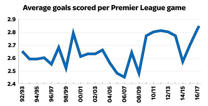
However, due to the low-scoring nature of games (less than 3 goals per game on av-
erage in the English Premier League in the past 15 years) (Fig.1.1), there is a random
element linked to the number of goals scored during a match. For instance, a team
with many scoring opportunities could be unlucky and convert none of their oppor-
tunities into goals, whereas a team with a single scoring opportunity could score a
goal. This makes match results an imperfect measure of a team’s performance and
therefore an incomplete metric on which to predict future results.
Figure 1.1: Average number of goals scored per game in the English Premier League [2]
A potential solution to this problem can be explored by using in-game statistics to
dive deeper than the simple match results. In the last few years, in-depth match
statistics have been made available, which creates the opportunity to look further
2Chapter 1. Introduction 1.3. OBJECTIVES than the match result itself. This has enabled the development of ’expected goals’ metrics which estimate the number of goals a team should have been expected to score in a game, removing the random element of goalscoring. The emergence of new Machine Learning techniques in recent years allow for better predictive performance in a wide range of classification and regression problems. The exploration of these different methods and algorithms have enabled the devel- opment of better models in both predicting the outcome of a match and the actual score. 1.3 Objectives This project aims to extend the state of the art by combining two popular and mod- ern prediction methods, namely an expected goals model as well as attacking and defensive team ratings. This has become possible thanks to the large amount of data that is now being recorded in football matches. Different Machine Learning models will be tested and different model designs and hypotheses will be explored in order to maximise the predictive performance of the model. In order to generate predictions, there are some objectives that we need to fulfill: Firstly, we need to find good-quality data and sanitize it to be used in our models. In order to do so, we will need to find suitable data sources. This will allow us to have access to a high number of various statistics to use, compared to most of the past research that has been done on the subject where only the final result of each match is taken into account. The main approach we will take is to build a model for expected goal statistics in order to better understand a team’s performance and thus to generate better pre- dictions for the future. To build this model, we will test different Machine Learning techniques and algorithms in order to obtain the best possible performance. We will be able to use data for shots taken and goals scored such as the location on the pitch or the angle to goal to estimate how many goals a team would have been expected to score during the game, and reduce the impact of luck on the final match result. In parallel to this, we will generate and keep track of team ratings as football matches are played to take into account the relative strength of the opposition, in a similar way to the popular ELO rating system. This will allow us to better gauge a team’s current level and in consequence to generate better predictions for future games. These two key project objectives are presented in Fig.1.2. An important part of this project will be to build a suitable Machine Learning train- ing and testing pipeline to be able to test new algorithms, with new features, and 3
1.3. OBJECTIVES Chapter 1. Introduction
Figure 1.2: Key project objectives to generate predictions
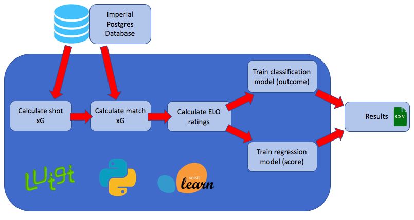
compare it to other models with relative ease, which will result in a general project
workflow illustrated in Fig.1.3.
Figure 1.3: Project Workflow
Finally, our models will be assessed against benchmark predictive methods including
bookmakers’ odds, using different performance metrics. A successful outcome for the
project would be the creation of both a classification model capable of predicting a
future game’s outcome, and a regression model capable of predicting a future game’s
score, whose predictive performance compare favourably to different benchmark
methods.
4Chapter 1. Introduction 1.4. CHALLENGES
1.4 Challenges
We face a number of challenges on the path to achieving the objectives we have set
out:
• Data availability & quality: Finding a public database of football data with
the necessary statistical depth to generate expected goals metrics is an essen-
tial part of the project. However, the leading football data providers do not
make their information publicly available. We will need to scour various pub-
lic football databases to find one that is suitable for us to use. The alternative
approach in the case where we do not find a suitable database would be to
find websites displaying the required data and using web scraping techniques
to create our own usable database.
• Research and understanding of prediction landscape: In order to design
our models and test different hypotheses, we will need to undertake a thor-
ough background research of prediction techniques and develop a mathemati-
cal understanding of various Machine Learning algorithms that can be used for
our predictions.
• Testing different models and parameters: An important challenge will be
to make the model training and testing tasks as quick and easy as possible, in
order to test and compare different models. A robust pipeline will have to be
built to enable us to find the best possible models.
1.5 Contributions
• An exploration of the Machine Learning landscape as well as past research in
sports predictions, presented in Chapter 2.
• A prepared and usable dataset containing all necessary statistics to generate
expected goal metrics and calculate team ELO ratings, presented in Chapter 3.
• A model training and testing pipeline allowing us to quickly and easily generate
performance metrics for different models and hypotheses, presented in Chapter
5.
• A classification model to predict match outcomes and a regression model to
predict match results, presented in Chapters 4 and 6.
• An assessment of our models’ performance against benchmark methods, pre-
sented in Chapter 7.
5Chapter 2
Background
2.1 Football Rules & Events
In this section, we will quickly present the rules of football, different match events
and possible outcomes.
• Simplified football rules:
– Football is a game played with two opposing teams of 11 players and a
ball, during 90 minutes.
– On each side of the pitch, a team has a target called the goal in which
they attempt to put the ball.
– Scoring a goal gives a team 1 point.
– The team with the largest number of points at the end of the game wins
the match.
– If both teams have scored the same number of goals, the game ends in a
draw.
• Domestic leagues competition format:
– Each European country usually has a domestic league where clubs play
against each other.
– There are usually 20 teams in each league, with each team playing the
others twice, once at their stadium (’home’ match) and once at the oppos-
ing team’s stadium (’away’ match).
– Winning a match gives a team 3 points, a draw gives each team 1 point.
– The team with the highest number of points at the end of the season wins
the league.
• Main match events:
– Goals: a goal is scored when the ball enters the opposing team’s goal.
6Chapter 2. Background 2.2. MACHINE LEARNING TECHNIQUES
– Shots: a shot is when a player hits the ball towards the opposing team’s
goal with the intention of scoring. There are many different kinds of shots,
hit with different parts of the body or from different distances and angles.
– Passes: a pass is when a player hits the ball towards another player of his
team.
– Crosses: a cross is when a player hits the ball from the side of the pitch
towards the opposing team’s goal with the intention of passing the ball to
one of his teammates.
– Possession: the possession represents the fraction of the time that a team
controls the ball in the match.
– Penalties & Free Kicks: free kicks happen when a foul is committed by
the opposing team on the pitch. In that case, the team that conceded
the foul can play the ball from where the foul has happened. If the foul
happens inside the penalty box (the zone near the goal), a penalty is
awarded: the team that conceded the foul can shoot at goal from close
range without anyone from the opposing team around.
– Cards: cards are awarded whenever the referee deems a foul to be suit-
ably important. Yellow cards are awarded for smaller fouls and do not
have a direct consequence. However, two yellow cards collected by the
same player result in a red card. If a player collects a red card, they
have to leave the pitch, leaving their team with one less player. Red cards
can also be directly obtained if a dangerous foul is committed or in other
specific circumstances.
– Corners: corners are awarded to the opposing team when a team hits the
ball out of the pitch behind their goal. In this case, the ball is placed on
the corner of the pitch and can be hit without any other player around.
2.2 Machine Learning Techniques
In this section, we will present an overview of popular supervised Machine Learning
techniques, for its subsets of classification and regression.
Supervised learning is the task of learning a function that maps input data to output
data based on example input-to-output pairs. Classification happens when the out-
put is a category, whereas regression happens when the output is a continuous num-
ber. In our case, we want to predict the outcome category (home win/draw/away
win) or the number of goals scored by a team (continuous number), so we are only
interested in the supervised learning landscape of Machine Learning. We have sum-
marised some popular supervised learning methods in Fig.2.1, which we will now
cover in more detail.
72.2. MACHINE LEARNING TECHNIQUES Chapter 2. Background
Figure 2.1: Overview of supervised Machine Learning techniques
2.2.1 Generalized Linear Models
Generalized Linear Models are a set of regression methods for which the output
value is assumed to be a linear combination of all the input values (Fig.2.2).
Figure 2.2: Linear Regression technique [3]
8Chapter 2. Background 2.2. MACHINE LEARNING TECHNIQUES
The mathematical formulation of the regression problem is:
y= 0 + 1 x1 + ... + m xm +✏
where:
• y is the observed value/dependent variable
• the xk are the input values/predictor variables
• the k are the weights that have to be found
• ✏ is a Gaussian-distributed error variable
Linear Regression fits a linear model with weights ˆ = ( ˆ1 , ..., ˆm ) by minimizing
the residual sum of squares between the actual responses Y in the dataset and the
predicted responses X where X is the matrix of input variables in the dataset. This
is the Ordinary Least Squares method:
ˆ = min kX Y k2
Once the model has been fitted with the best possible weight , the Linear Regres-
sion model can generate a continuous output variable given a set of input variables.
On the other hand, Logistic Regression is a classification model for a binary output
variable problem. Indeed, the output variable of the model represents the log-odds
score of the positive outcome in the classification.
ln( 1 p(x)
p(x)
)= 0 + 1 x1 + ... + m xm
The log-odds score is a continuous variable which is used as input in a logistic func-
tion (Fig.2.3):
1
(z) = 1+e z
The logistic function outputs a number between 0 and 1 which is chosen to be the
probability of the positive classification outcome given the input variables. Setting
and optimizing a cut-off probability allows for classification decisions to be made
when presented with new input variables.
Generalized Linear Models are a popular technique as they are easy to implement
and, in many classification or regression problems, assuming linearity between pre-
dictor variables and the outcome variable is sufficient to generate robust predictions.
In addition to this, the fitted coefficients are interpretable, meaning that we can un-
derstand the direction and magnitude of association between each predictor variable
and the outcome variable.
92.2. MACHINE LEARNING TECHNIQUES Chapter 2. Background
Figure 2.3: Logistic function [4]
However, using Generalized Linear Models can also have some disadvantages: the
assumption that the input variables and output variable are linearly connected does
not always fit the problem and can be too simple. Furthermore, if the input variables
are highly-correlated, the performance of the model can be quite poor.
2.2.2 Decision Trees
Decision Trees are a popular Machine Learning technique to link input variables,
represented in the tree’s branches and nodes, with an output value represented in
the tree’s leaves. Trees can both be used in classification problems, by outputting
a category label, or in regression problems, by outputting a real number. Decision
Trees can be fitted using different algorithms, including the CART or ID3 decision
tree algorithms which are the most popular. These algorithms use a mix of greedy
searching and pruning so that the tree both fits and generalizes the data to new in-
put/output pairs.
Decision Trees have the advantage that they scale very well with additional data,
they are quite robust to irrelevant features and they are interpretable: the choices
at each node allow us to understand the impact of each predictor variable towards
the outcome. However, decision trees can often become inaccurate, especially when
exposed to a large amount of training data as the tree will fall victim to overfitting.
This happens when the model fits the training data very well but is not capable of
generalizing to unseen data, thus resulting in poor predictive performance.
Random Forests operate by building a large amount of decision trees during training,
taking a different part of the dataset as the training set for each tree. For classifi-
10Chapter 2. Background 2.2. MACHINE LEARNING TECHNIQUES
cation problems, the final output is the mode of the outputs of each decision tree,
whereas for regression problems, the mean is taken. This technique is illustrated in
Fig.2.4.
This results in a model with much better performance compared to a simple decision
tree, thanks to less overfitting, but the model is less interpretable as the decisions at
the nodes of the trees are different for each tree.
Figure 2.4: Random Forest technique [5]
2.2.3 Probabilistic classification
Probabilistic classifiers are Machine Learning methods capable of predicting the
probability distribution over classes given input variables.
One of the most popular probabilistic classifiers is the Naive Bayes classifier. It is
a probabilistic classification method based on the ’naive’ assumption that every two
different features are independent, thus enabling the use of Bayes’ Theorem:
P (y)P (x1 ,...,xn |y)
P (y|x1 , ..., xn ) = P (x1 ,...,xn )
where:
• y is the target class
• the xi are the predictor (input) variables
112.2. MACHINE LEARNING TECHNIQUES Chapter 2. Background
Using the independence assumption, this leads to the following:
Qn
P (y|x1 , ..., xn ) / P (y) i=1 P (xi |y)
MAP (Maximum A Posteriori) estimation enables the creation of a decision rule (rule
to choose the class to return as output) by choosing the most probable hypothesis.
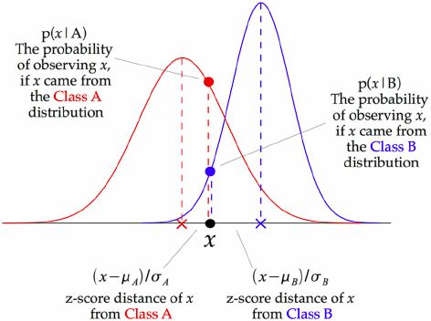
For Gaussian Naive Bayes, the likelihood P (xi |y) of the features is assumed to follow
a Gaussian distribution, as illustrated in Fig.2.5:
(xi µy )2
P (xi |y) = p 1 2
exp( 2 y2
)
2⇡ y
where the y and µy parameters are estimated using Maximum Likelihood Estima-
tion.
The advantages of using Naive Bayes classifiers is that they are highly scalable when
presented with large amounts of data: indeed, they take an approximately linear
time to train when adding features. However, even though the classifier can be
robust enough to ignore the naive assumption, the predicted probabilities are known
to be somewhat inaccurate.
Figure 2.5: Gaussian Naive Bayes method [6]
12Chapter 2. Background 2.2. MACHINE LEARNING TECHNIQUES
2.2.4 Lazy learning
Lazy learning is a Machine Learning technique for which no model is actually built
but the training data is generalized when new inputs are given. They are known to
be best for large sets of data with a small number of features.
The K-nearest-neighbors algorithm is a lazy learning method for both classification
and regression that takes the k nearest training examples in the feature space and
outputs:
• for classification: the most common class among the k neighbors
• for regression: the average of the values for the k neighbors
The best choice for the k parameter depends on the training data set. Indeed, a
higher value reduces the effect of noise in the data but makes the approximation
less local with regards to other training data points. A classification example using
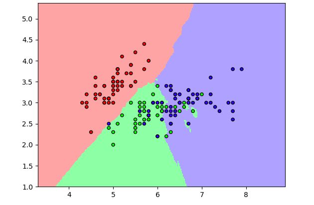
the k-Nearest Neighbors method is illustrated in Fig.2.6.
Figure 2.6: k-Nearest-Neighbors classification [7]
The main advantage of lazy learning methods is that the target function is approx-
imated locally, which means that it is sensitive to the local structure of the training
data. This allows these methods to easily deal with changes in the underlying data
classification or regression distributions. However, these methods come with some
drawbacks: space is required to store the training dataset as the algorithm will run
through all training data examples to find those that are closest to the input values.
This makes these techniques quite slow to evaluate when testing.
132.2. MACHINE LEARNING TECHNIQUES Chapter 2. Background
2.2.5 Support Vector Machines
Support Vector Machines (SVMs) are Machine Learning models for both classifica-
tion and regression. An SVM model represents the training data as points in space so
that examples falling in different categories are divided by a hyperplane (see Fig.2.7)
that is as far as possible from the nearest data point.
Figure 2.7: SVM Hyperplane for classification [8]
New inputs are mapped in the same way as the training data and classified as the
category they fall into (which side of the hyperplane). When the data is not linearly
separable, the kernel trick can be used, by using different possible kernel functions
such as Radial Basis Functions (RBF) or polynomial functions, in order to map the
data into high-dimensional feature spaces and find a suitable high-dimensional hy-
perplane.
The above classification problem can be extended to solving regression problems in
a similar way, by depending only on a subset of the training data to generate a re-
gression prediction.
Advantages for using Support Vector Machines include that they are effective in high-
dimensional spaces, that they are memory efficient thanks to the use of a subset of
training points in the decision function, and finally that they are versatile through
the use of different possible kernel functions. On the other hand, using SVMs can
have some disadvantages: they do not directly provide probability estimates for clas-
sification problems, and correctly optimising the kernel function and regularization
term is essential to avoid overfitting.
14Chapter 2. Background 2.2. MACHINE LEARNING TECHNIQUES
2.2.6 Neural Network models
Neural Networks, also known as Artificial Neural Networks (ANNs), are systems that
are based on a collection of nodes (neurons) that model at an algorithmic level the
links between neurons in the human brain.
Each neuron can receive a signal from neurons and pass it on to other neurons.
Two neurons are connected by an edge which has a weight assigned to it, which
models the importance of this neuron’s input to the other neuron’s output. A neural
network is usually composed of an input layer, with one neuron per input variable
for the model, an output layer, composed of a single neuron which will give the
classification or regression result, and a number of hidden layers between the two,
containing a variable number of neurons in each layer. Fig.2.8 illustrates the archi-
tecture of a neural network with one hidden layer.
Figure 2.8: Neural Network diagram [9]
A neuron which receives an input pj from another neuron then computes its activa-
tion value through its activation function f : aj = f (pj ). The neuron’s output oj is
then generated through its output function fo such that oj = fo (aj ).
This leads us to the propagation function which calculates the input pj that a neuron
j receives in the network:
P
pj = i oi wij where wij is the weight between neurons i and j
Training the Neural Network model involves setting the correct weight between each
152.3. PAST RESEARCH Chapter 2. Background
two neurons in the system. This is done through the back-propagation algorithm
which inputs a new training example, calculates gradient of the loss function (a
function which quantifies the error between the Neural Network prediction and the
actual value) with respect to the weights and updates the weights from the output
layer all the way back to the input layer:
@C
wij (t + 1) = wij (t) + ⌘ @w ij
where:
• ⌘ is the learning rate and determines the magnitude of change for the weights
• C is the cost/loss function which depends on the learning type and neuron
activation functions used
The advantages in using Neural Networks as classification or regression models are
that they usually achieve a high level of predictive accuracy compared to other tech-
niques. However, they require a very large amount of training data to optimise the
model. In addition to this, neural networks are not guaranteed to converge to a
single solution and therefore are not deterministic. Finally, Neural Networks are not
interpretable: indeed, there are in general too many layers and neurons to under-
stand the direction and magnitude of association of each input variable with the
output variable through the different weights.
2.3 Past Research
We have separated the past research on football predictions in three categories.
Firstly, we will look at the general landscape of football predictions and the Machine
Learning techniques that have previously been used. Secondly, we will concentrate
on research linked to using team ratings to improve predictions. Finally, we will talk
about the papers that present models estimating the expected goals that a team is
estimated to have obtained.
2.3.1 Football prediction landscape
Generating predictions for football scores has been an important research theme
since the middle of the 20th century, with the first statistical modelling approaches
and insights coming from Moroney (1956) [10] and Reep (1971) [11] who used
both the Poisson distribution and negative binomial distribution to model the amount
of goals scored in a football match, based on past team results.
However, it was only in 1974 that Hill proved that match results are not solely based
on chance, but can be modeled and predicted using past data [12].
The first breakthrough came from Maher [13] in 1982 who used Poisson distribu-
tions to model home and away team attacking and defensive capabilities, and used
16Chapter 2. Background 2.3. PAST RESEARCH
Figure 2.9: Poisson distribution for values of and k [15]
this to predict the mean number of goals for each team. Following this, Dixon and
Coles [14] (1997) were the first to create a model capable of outputting probabilities
for match results and scores, again following a Poisson distribution.
The Dixon and Coles model is still seen as a traditionally successful model, and we
will use it as a benchmark against the models that we will be creating.
The Dixon and Coles model is based on a Poisson regression model, which means
that an expected number of goals for each team are transformed into goal probabil-
ities following the Poisson distribution (illustrated in Fig.2.9):
k
P (k goals in match)= e k!
where represents the expected number of goals in the match.
The Poisson distribution enables the calculation of the probability of scoring a certain
number of goals for each team, which can then be converted into score probabilities
and finally into match outcome probabilities.
Based on past results, the Dixon and Coles model calculates an attacking and de-
172.3. PAST RESEARCH Chapter 2. Background
fensive rating for each team by computing Maximum Likelihood estimates of these
ratings on past match results and uses a weighting function to exponentially down-
weight past results based on the length of time that separates a result from the actual
prediction time.
Rue and Salveson [16] (2000) chose to make the offensive and defensive parame-
ters vary over time as more results happen, then using Monte Carlo simulation to
generate predictions. In 2002, Crowder et al. [17] followed up on their work to
create a more efficient update algorithm.
At the beginning of the 21st century, researchers started to model match results
(win/draw/loss) directly rather than predicting the match scores and using them to
create match result probabilities. For example, Forrest and Simmons (2000) [18]
used a classifier model to directly predict the match result instead of predicting the
goals scored by each time. This allowed them to avoid the challenge of interdepen-
dence between the two teams’ scores.
During the same year, Kuypers [19] used variables pulled from a season’s match re-
sults to generate a model capable of predicting future match results. He was also
one of the first to look at the betting market and who tried to generate profitable
betting strategies following the model he developed.
We have therefore seen that past research have tried to predict actual match scores
as well as match results. It would be interesting in this project to look at the perfor-
mance of generating a classification model for match outcome against a regression
model for match scores.
We will now take a look at more recent research done on the subject, with the use
of modern Machine Learning algorithms that will be interesting for us to investigate
when trying different predictive models.
In 2005, Goddard [20] tried to predict football match results using an ordered probit
regression model, using 15 years of results data as well as a few other explanatory
variables such as the match significance as well as the geographical distance between
the two teams. It was one of the first papers to look at other variables than actual
match results. He compared the model predictions with the betting odds for the
matches and found that there was the possibility of a positive betting return over
time. Like Goddard, we will want to use other explanatory variables in our model
than only match results, which will allow us to use different sets of features to try
obtaining the best model possible.
It is also interesting to look at the algorithms used for predictions in other team
sports: for example, in 2006, Hamadani [21] compared Logistic Regression and
SVM with different kernels when predicting the result of NFL matches (American
Football).
18Chapter 2. Background 2.3. PAST RESEARCH More recently, Adam (2016) [22] used a simple Generalised Linear Model, trained using gradient descent, to obtain match predictions and simulate the outcome of a tournament. He obtained good results, even with a limited set of features, and recommends to add more features and to use a feature selection process, which is something that will be interesting for us to do in this project considering the number of different features that will be available to us. Tavakol (2016) [23] explored this idea even further: again using a Linear Model, he used historical player data as well as historical results between the two teams going head to head in order to generate predictions. Due to the large number of features available, he used feature extraction and aggregation techniques to reduce the number of features to an acceptable level to train a Linear Model. There are multiple ways to reduce the number of features to train a Machine Learn- ing model: for instance, Kampakis [24] used a hierarchical feature design to pre- dict the outcome of cricket matches. On the other hand, in 2015, Tax et al. [25] combined dimensionality reduction techniques with Machine Learning algorithms to predict a Dutch football competition. They came to the conclusion that they ob- tained the best results for the PCA dimensionality reduction algorithm, coupled with a Naive Bayes or Multilayer Perceptron classifier. It will be interesting for us to try different dimensionality reduction techniques with our Machine Learning algorithms if we have a large number of features we choose to use. This also shows us that a large amount of data might not be required to build a Neural Network model and achieve interesting results. Bayesian networks have been tested in multiple different recent research papers for predicting football results. In 2006, Joseph [26] built a Bayesian Network built on expert judgement and compared it with other objective algorithms, namely Decision Tree, Naive Bayesian Network, Statistics-based Bayesian Network and K-nearest- neighbours. He found that he obtained a better model performance for the Network built on expert judgement, however expert knowledge is needed and the model quickly becomes out of date. Another type of Machine Learning technique that has been used for a little longer is an Artificial Neural Network (ANN). One of the first studies on ANN was made by Purucker in 1996 [27] to predict NFL games, who used backpropagation to train the network. One of the limitations of this study was the small amount of features used to train the network. In 2003, Kahn [28] extended the work of Purucker by adding more features to train the network and achieved much better results, confirming the theory that Artificial Neural Networks could be a good choice of technique to build sports predictive models. Hucaljuk et al. (2011) [29] tested different Machine Learning techniques from mul- tiple algorithm families to predict football scores: 19
2.3. PAST RESEARCH                                             Chapter 2. Background

   • Naive Bayes (probabilistic classification)

   • Bayesian Networks (probabilistic graphical model)

   • LogitBoost (boosting algorithm)

   • K-nearest-neighbours (lazy classification)

   • Random Forest (decision tree)

   • Artificial Neural Networks

They observed that they obtained the best results when using Artificial Neural Net-
works. This experiment is espacially interesting to us as we will want to test different
algorithms in the same manner, to obtain the one that works the best for our data
and features.

By looking at the past research done on the subject of building models to predict
football match outcomes, we have been able to gain interesting information on the
different techniques we should try using as well as the potential pitfalls we should
avoid.

2.3.2    ELO ratings
We will now look at two areas of research that are especially important considering
the objective of our project: firstly, we will want to look at how team ratings have
previously been used to improve predictions.

The most famous rating system, still used today, was invented in 1978 by Elo [30]
to rate chess players. The name ”ELO rating” was kept for future uses, such as Buch-
dahl’s 2003 paper [33] on using ELO ratings for football to update teams’ relative
strength. These types of rating have also been used for other sports predictions, such
as tennis. Indeed, Boulier and Stekler (1999) [31] used computer-generated rank-
ings to improve predictions for tennis matches, while Clarke and Dyte (2000) [32]
used a logistic model with the difference in rankings to estimate match probabilities.

In 2010, Hvattuma used an ELO system [34] to derive covariates used in regression
models in the goal of predicting football match outcomes. He tested two different
types of ELO ratings, one taking in account the match result (win/loss/draw) and
another only taking the actual score in account. He used different testing bench-
marks to evaluate his predictions, which enabled him to see that he obtained better
results using ELO ratings than the other benchmarks he ran his model against. Rel-
ative team strength ratings are very important to us in this project to encode past
information and continuously update each team’s relative strength as new results
are added to the model.

                                                                                     20
Chapter 2. Background 2.3. PAST RESEARCH
We will want to explore different possibilities of keeping track and updating these
team ratings over time. Multiple approaches have already been explored: to gener-
ate predictions for the football Euro 2016 tournament, Lasek (2016) [35] compared
using ordinal regression ratings and using least squares ratings, combined with a
Poisson distribution, to generate predictions and simulate the tournament a large
number of times using Monte Carlo simulations. Viswanadha et al. (2017) [36] used
player ratings rather than team ratings to predict the outcome of cricket matches
using a Random Forest Classifier. Using player data to calculate relative player
strengths and improve our model could be a potential extension to this project. Fi-
nally, in 2013, Fenton [37] came up with a new type of team rating, called pi-rating.
This rating dynamically rates teams by looking at relative differences in scores over
time. There are clearly different ways of evaluating relative team strength and weak-
ness, and we will need to try different techniques for this project to try and obtain
the best predictions we can.
2.3.3 Expected goals (xG) models
The second theme that is important to us for this project is building an expected
goals model. This is a quite modern concept that aims to analyse match data to un-
derstand how many goals a team should have scored considering the statistics that
have been observed during the match. Using an expected goals model enables us
to eliminate some of the randomness that is associated with actual goals scored and
get a better picture of a team’s performance, and therefore strength.
In 2012, MacDonald [38] created an expected goals model to evaluate the perfor-
mance of NHL (Hockey) matches, using two metrics:
• The Fenwick rating (shots and missed shots)
• The Corsi rating (shots, missed shots and blocked shots)
This enabled the evaluation of a team’s performance to understand if, for example,
they were wasteful with their goal opportunities, or if they did not manage to create
enough goalscoring opportunities. Very good results were obtained for this expected
goals model, with more efficient estimates for future results. A possible extension
for this paper would be to use the opponent’s data to calculate the expected goals.
That is exactly what we will be trying to do with football: using both teams’ data to
understand how many goals each team were expected to score in a match, and use
this value to improve future predictions.
In 2015, Lucey [40] used features from spatio-temporal data to calculate the likeli-
hood of each shot of being a goal. This includes shot location, defender proximity,
game phase, etc. This allows us to quantify a team’s effectiveness during a game and
generate an estimation for the number of goals they would have been expected to
score. This example is particularly interesting for us, as we have geospatial data for
shots and goals scored in matches. We will use that data to build an advanced ex-
pected goals model to better understand how a team has actually performed during
212.3. PAST RESEARCH Chapter 2. Background
the game.
Similarly, Eggels (2016) [39] used classification techniques to classify each scoring
opportunity into a probability of actually scoring the goal, using geospatial data
for the shot as well as which part of the body was used by the player. Difference
classification techniques were tested including logistic regression, decision trees and
random forest. We will also need in this project to test different methods of quanti-
fying the probability of scoring a goal for each opportunity.
Finally, one of the most interesting examples for out project comes from a website
named FiveThirtyEight [41], who combine an expected goals model with a team
rating system to predict the outcome of future football matches. In essence, they
keep an offensive and defensive rating for each time depending on an average of
goals scored and expected goals that are recorded in each game. This allows them
to forecast future results and run Monte Carlo simulations to try and predict compe-
tition winners. It is interesting to note that the weight given to the expected goals
decrease if a team is leading at the end of a match, which would be an hypothesis
for us to explore.
For our project, we will take inspiration from these methods, but we will improve the
expected goals model by testing different Machine Learning algorithms and adding
features in order to try and output the best possible predictions.
22Chapter 3
Dataset
3.1 Data origin
We have obtained a dataset from the Kaggle Data Science website called the ’Kaggle
European Soccer Database’ [42]. This database has been made publicly available
and regroups data from three different sources, which have been scraped and col-
lected in a usable database:
• Match scores, lineups, events: http://football-data.mx-api.enetscores.com/
• Betting odds: http://www.football-data.co.uk/
• Players and team attributes from EA Sports FIFA games: http://sofifa.com/
It includes the following:
• Data from more than 25,000 men’s professional football games
• More than 10,000 players
• From the main football championships of 11 European countries
• From 2008 to 2016
• Betting odds from various popular bookmakers
• Team lineups and formations
• Detailed match events (goals, possession, corners, crosses, fouls, shots, etc.)
with additional information to extract such as event location on the pitch (with
coordinates) and event time during the match.
We will only be using 5 leagues over two seasons as they possess geographical data
for match events that we will need to build our expected goals models:
• English Premier League
• French Ligue 1
233.2. DATA PRE-PROCESSING Chapter 3. Dataset
• German Bundesliga
• Spanish Liga
• Italian Serie A
We will only be using data from the 2014/2015 as well as 2015/2016 seasons as they
are the most recent seasons available in the database and the only ones containing
the data that we need.
This gives us usable dataset of:
• 3,800 matches from the top 5 European leagues
• 88,340 shots to analyse
• More than 100 different teams
3.2 Data pre-processing
An important step before building our model is to analyse and pre-process the data
to make sure that it is in a usable format for us to use when training and testing
different models.
Three pre-processing steps were taken in order to achieve this:
• Part of the data that we needed, namely all match events such as goals, posses-
sion, corners, etc. was originally in XML format in the database. We therefore
built a script in R to extract this data and store it in new tables, linked to the
’Matches’ table thanks to a foreign key mapping to the match ID. An extract of
the XML for a goal in one match is presented below:
n
1
1
406
18
67
35
35345
header
26777
24Chapter 3. Dataset 3.3. DATA FEATURES
1
9826
3647567
200
goal
n
• Some data elements were set to NULL, which led to us deleting some unusable
rows and in other cases to us imputing values to be able to use the maximum
possible amount of data. For instance, the possession value was missing for
some games, so we entered a balanced value of 50% possession for each team
in this case.
• Finally, having extracted the geographical coordinates for each shot in the
dataset, we generated distance and angle to goal values which we added to
our goals and shots database tables.
The following formula was used to generate the distance to goal of a shot,
where the coordinates of the goal are (lat=0, lon=23):
p
D(lat, lon) = lat2 + (lon 23)2
The following formula was used to generate the angle of a shot:
A(lat, lon) = tan 1 ( |lonlat23| )
3.3 Data features
A simplified diagram of the database structure and features is presented in Fig.3.1.
We will now present the different tables and features that we have in our database
and that we can use in our models:
• Matches table
– ID
– League ID
– Season
– Date
– Home team ID
– Away team ID
253.3. DATA FEATURES Chapter 3. Dataset
Figure 3.1: Structure of the Database
– Home team goals scored
– Away team goals scored
– Home team possession
– Away team possession
– Home win odds
– Draw odds
– Away win odds
• Events tables:
Here is a list of the different match events tables that we have extracted:
– Goals
– Shots on target
– Shots off target
– Corners
– Crosses
– Cards
– Fouls
For each of these match event tables, we have the following features:
– ID
– Type
26Chapter 3. Dataset 3.3. DATA FEATURES
– Subtype
– Game ID
– Team ID
– Player ID
– Distance to goal (only for goals and shots)
– Angle to goal (only for goals and shots)
– Time elapsed
Extracts of the database and row values examples are available in the Appendix.
27Chapter 4
Design
In this chapter, we will present the general design of our model and the choices we
have made.
Our model is a mixture of multiple regression and classification algorithms used to
generate different metrics that are finally used as inputs for our classification model
(for match outcomes) and regression model (for match scores).
4.1 Model components
In this section, we will introduce the different components of our model and explain
their role.
A diagram of our different components and how they are linked is presented in
Fig.4.1.
Figure 4.1: Diagram of model components
28Chapter 4. Design 4.2. MODEL CHOICES
We have five main model components which we will present one by one:
• Shot xG generation:
This component’s objective is to generate an expected goal value for each shot
representing the probability that the shot results in a goal, with some adjust-
ments to reflect specific match situations.
• Match xG generation:
This component’s objective is to generate a shot-based expected goals value for
each match by looking at the expected goals values for each shot during that
match. In addition to this, a non-shot-based expected goals value is generated
using match information other than shots.
• ELO calculation:
This component’s objective is to generate offensive and defensive team ELO
ratings after each match using expected goals values and the actual perfor-
mance. ELO ratings are recalculated after each match and the team ratings are
stored for use in our predictive classification and regression models.
• Classification model training:
This component’s objective is to train and test a classification model capable of
taking two teams’ ELO ratings and generating a prediction for a match between
these two teams between a home team win, a draw and an away team win.
• Regression model training:
This component’s objective is to train and test a regression model capable of
taking two teams’ ELO ratings and generating a prediction for the expected
number of goals each team will score. These values are then used to generate
a prediction for the match outcome.
4.2 Model choices
We will now dive into more detail for each component of the model, presenting the
choices we have made and explaining how each value is obtained.
• Shot xG generation:
– To generate an expected goals value for each shot, we firstly take all shots
in our database, including goals, shots on target that did not result in a
goal (shots that were stopped on their way to goal by another player) and
shots off target (shot attempts that do not go in the direction of the goal.
– We then separate each shot into a specific category depending on the type
of shot:
⇤ ’Normal’ shots: lobs, shots from distance, deflected shots, blocked
shots, etc.
294.2. MODEL CHOICES Chapter 4. Design
⇤ Volleys (shots hit with the foot when the ball is still in the air)
⇤ Headers (shots hit with the head)
⇤ Direct free-kicks (shots that result from a free kick that can be directly
shot at goal)
⇤ Indirect free-kicks (shots that result from a free kick that cannot be
directly shot at goal)
⇤ Bicycle kicks (shots taken above the level of the shoulders)
⇤ Own goals (goals scored by players into their own net)
⇤ Penalties
– Next, we assign an outcome value of 1 to each shot that resulted in a goal,
and 0 to each shot that did not result in a goal.
– This allows us to build a separate classification model for each shot type,
taking as predictor variables the distance to goal and the angle to goal,
with the outcome variable reflecting if the shot resulted in a goal or not.
We have chosen to build a separate classification model for each shot type
as we make the assumption that each type of these goals have different
probabilities of resulting in a goal if taken from the same exact location
on the pitch.
– For each shot, we calculate the probability of scoring as an expected goals
value using the suitable classification model, entering as input the shot
distance and angle to goal, as illustrated by Fig.4.2.
Figure 4.2: Diagram of shot distance and angle used to predict xG
30Chapter 4. Design 4.2. MODEL CHOICES
– Once we have our expected goals value for a shot, we proceed with an ad-
justment based on if the team is already leading and by how many goals.
We decide to make different adjustments if a team is winning by a single
goal, with the match final outcome still in the balance, and when a team
is winning by two goals or more, making the lead more comfortable for
the side that is winning. Adjusting the expected goals value is done to
reflect the fact that a team that is losing will become more attacking to try
and equalise or gain a result from the match, thus making it easier for the
winning team to attack and score goals, and making the shot worth less
than if the teams had the same number of goals for example.
We therefore decide to set a time t in the match after which the value of
a shot will decrease linearly until the end of the game towards a weight
k between 0 and 1. We will later try different times for which to start
decreasing shot values, with the hypothesis that the time where substitu-
tions are usually made could be a good starting point as managers often
bring on a more attacking player for a more defensive one in order to
catch up in the score. We will also try different values k if a team is lead-
ing by 1 goal or by 2 goals and more. Fig.4.3 illustrates our hypothesis by
showing the value of a goal as the game is progressing.
Figure 4.3: Diagram of value of shot xG over time when team is leading
– Finally, we proceed with a final adjustment, which is to decrease the value
of a shot by a certain coefficient if the player’s team has a higher number
of players on the pitch due to a red card given to one of the opposing
team’s players. This is due to the fact that a team with less players will
have on average a worse performance than if the two teams have the same
number of players, making it easier to attack and score for the opponent.
We also decide to increase the value of a shot by another coefficient if the
player’s teams have a lower number of players on the pitch, for the same
reason as mentioned above.
314.2. MODEL CHOICES Chapter 4. Design
• Match xG generation:
– Firstly, for each match, we sum of each team’s shot expected goals values
to generate a shot-based expected goals value for each team at the end of
a match.
– We also decide to build a non-shot-based expected goals metric for each
team by evaluating other information than shots:
⇤ possession
⇤ number of corners
⇤ number of crosses
⇤ number of yellow cards
⇤ number of yellow cards for the opponent
⇤ number of fouls
⇤ number
– We therefore decide to train a regression model which takes as input
these previously mentioned statistics for each team and takes as output
the number of actual goals the team has scored. We take this decision as
dangerous situations on the pitch that can result in goals can often not
lead to a shot being taken. We believe that using other information al-
lows us to better assess a team’s performance and their likelihood to score
goals.
– Once we have built this regression model, we look at each match and
generate a non-shot-based expected goals metric for the home team and
for the away team depending on their in-match statistics.
– Both the shot-based and non-shot-based expected goal values will be used
to recalculate ELO ratings after each match.
• ELO calculation:
– Our main method for ELO calculation is to store team ratings and modify
the ratings after each match has been completed, in order to keep a metric
of team strength and weakness.
– Each team will possess 6 different ratings that will be stored and updated:
⇤ General offensive rating
⇤ General defensive rating
⇤ Home offensive rating
⇤ Away offensive rating
⇤ Home defensive rating
⇤ Away defensive rating
– Each offensive rating represents the number of goals the team would be
expected to score against an average team at that point in time, while
each defensive rating represents the number of goals the team would be
expected to conceded against an average team at that point in time.
32You can also read