ARMCHAIR FANS: NEW INSIGHTS INTO THE DEMAND FOR TELEVISED SOCCER - WORKING PAPER IN ECONOMICS - BABATUNDE BURAIMO DAVID FORREST IAN G. MCHALE J.D ...

Working Paper in Economics

 # 202020

 July 2020

ARMCHAIR FANS: NEW INSIGHTS
 INTO THE DEMAND FOR
 TELEVISED SOCCER

 Babatunde Buraimo
 David Forrest
 Ian G. McHale
 J.D. Tena

https://www.liverpool.ac.uk/management/people/economics/
© authors

ARMCHAIR FANS: NEW INSIGHTS INTO THE DEMAND FOR TELEVISED SOCCER
 by

 Babatunde Buraimo
 David Forrest
 Ian G. McHale
 and
 J.D. Tena

 July, 2020

Buraimo: Senior Lecturer, Centre for Sports Business, University of Liverpool Management School, Liverpool,
L69 7ZH, United Kingdom. Phone +44-1517953536, E-mail b.buraimo@liverpool.ac.uk

Forrest: Professor, Centre for Sports Business, University of Liverpool Management School, Liverpool, L69
7ZH, United Kingdom. Phone +44-1517950679, E-mail david.forrest@liverpool.ac.uk

McHale: Professor, Centre for Sports Business, University of Liverpool Management School, Liverpool, L69
7ZH, United Kingdom. Phone +44-1517952178, E-mail ian.mchale@liverpool.ac.uk

Tena: Senior Lecturer, Centre for Sports Business, University of Liverpool Management School, Liverpool, L69
7ZH, United Kingdom. DiSea & CRENOS, Università di Sassari, 07100, Sassari, Italy. Phone +44-1517953616,
E-mail jtena@liverpool.ac.uk

I. INTRODUCTION

 The first journal article modelling television audience demand for sport (Forrest,

Simmons and Buraimo 2005) focussed on the English Premier League (EPL). Since then

there has been a large successor literature on the same theme, embracing both soccer and

many other sports. Van Reeth (2020) provides a useful tabulation of studies to date.

 Studies in this strand of literature have obvious utility to various stakeholders.

Demand equations may be used to inform sports leagues as to the match characteristics

favoured by their audiences1, with implications for how best to design the formats of their

competitions and whether and how to manage issues such as competitive balance. They may

also be useful to broadcasters and advertisers, as forecasting tools to indicate likely audience

size for upcoming contests, relevant, for example, to pricing decisions for advertising slots.

And for economists they provide an opportunity to try to settle important issues in the

academic literature, such as the validity of the uncertainty of outcome hypothesis.2 This

should be easier to address in television demand studies than in stadium demand studies

because there is no complication from capacity constraints being reached and because the

dominance of home fans at physical venues makes it hard to separate out the influence of

tastes for uncertainty and tastes for a home win; a wider or national television audience will

have less skewed allegiances. Indeed, previous studies of television demand in the context of

the EPL have included ‘uncertainty’ in their title (Forrest, Simmons, and Buraimo 2004;

Buraimo and Simmons 2015; Cox 2018), indicating their primary motivation. The same

1
 In elite sports leagues, television audiences represent a much more lucrative source of revenue than stadium
attendees. For example, in season 2018-19, the EPL’s revenue from broadcasting rights was almost exactly four
times that from ‘match day income’ (Deloitte, 2020, p. 16). A similar business model applies in most American
Major League Sport and in cricket’s Indian Premier League.
2
 The uncertainty of outcome hypothesis proposes that interest in a particular sports event will be greater the
closer the contestants are in terms of their probability of winning. Its origins may be traced back to Rottenberg’s
(1956) notion of ‘competitive balance’. The latter may refer to uncertainty over seasonal outcomes or even to
the degree of dominance of particular clubs over time. However the term ‘uncertainty of outcome hypothesis’
generally refers to the level of the individual match.

 1

emphasis is found in the paper titles of television audience studies for other soccer leagues

(e.g. Pérez, Puente, and Rodríguez 2016; Schreyer, Schmidt and Torgler 2016) and for other

sports as well, for example Formula 1 motor racing (Schreyer and Torgler, 2018), cycling

(Van Reeth, 2013) and Australian Rules Football (Dang et al., 2015).

 Our reason for returning to such a well-trodden path in the literature is that we

acknowledge the utility and importance of the topic but believe that previous modelling has

been flawed and that, consequently, conclusions drawn from analyses to date are unsafe. In

particular, studies appear often to choose an inappropriate measure for the dependent

variable, audience size, and inadequate proxies for player quality and match significance,

archetypical conditions of demand included in modelling. In the next section, we shall

explain why previously adopted metrics fail meaningfully to capture the underlying concepts

of interest and why their use may lead to bias in the estimation of the key variables, including

outcome uncertainty. In section III, we propose alternative metrics, drawing on recent

advances in the field of sport analytics, advances which have not been reflected to any

significant extent in prior literature on mainstream topics in sports economics, such as

demand modelling. In sections IV and V, we present our econometric model and results,

demonstrating that use of our measures make a material difference to what can be concluded.

Section VI completes the paper by commenting on implications of our estimation results for

sport and for sports economics.

 2

II. PROBLEMS IN PRIOR LITERATURE

A. Empirical framework

 Studies of the television audience demand for soccer at the level of the match3 have

generally been framed in terms of a model such as:

(1) Ln(audience size)= f(player quality, outcome uncertainty, match significance,

controls).

 In the first paper to model audience size, Forrest, Simmons, and Buraimo (2005)

measured outcome uncertainty by the current difference in points per game between the

opposing clubs, adjusted to take account of the average points value of home advantage in the

league. They reported this measure as significant (though with small effect size).

Nevertheless it may be regarded as a fairly crude measure since it fails to take into account

factors influencing prospects for the match which are known to the prospective audience but

are not captured by summary statistics of the performances of the two clubs over the whole of

the season to date. For example, a club may have strengthened its team by entering the

transfer market in the January window precisely because it was dissatisfied with its current

position in the standings and its probability of a win in February may then be much greater

than its current points total would suggest.

 Most recent studies have therefore turned to the betting market to create an indicator

of uncertainty, presuming the market to be efficient, with odds capturing all current

information relevant to match prospects. Accordingly, the absolute difference in probabilities

of a win for the home and away clubs, as implied by the betting market, has been the most

3
 We account here only for papers aiming to explain variation in audience size across matches. A smaller
literature addresses causes of variation within matches, for soccer see Alavy, Gaskell, Leach, and Szymanski
(2010) and Buraimo, Forrest, McHale, and Tena (2020).

 3

common measure of outcome uncertainty adopted in recent studies of the demand for

televised soccer (e.g. Buraimo and Simmons 2015; Cox 2018; Caruso, Addesa, and Di

Domizio 2019; Bergmann and Schreyer 2019). In this paper we do not challenge this

consensus and will adopt the same metric in our modelling. However, we identify flaws in all

the other elements of (1) and will now address each in turn.

B. Measuring the dependent variable

 There is nothing to which to object in a decision to adopt the natural log of audience

size as the dependent variable. However, this begs the question (even if few authors answer

it): what is audience size? Van Reeth (2020) draws attention to how ambiguous this term can

be. In Europe at least, audience research agencies typically compile estimates for the number

of viewers at each minute of each programme of each television channel.4 Estimates of

audience size for a given programme can then refer to the average per-minute audience or to

the peak audience or to either expressed as a percentage of all viewing of programmes being

broadcast at the time. Nearly all published studies on soccer focus on average per-minute-

audience.5 But this still leaves ambiguity. The headline figure for audience size from the

audience research agency will relate to the whole programme whereas the match is only a

4
 A representative sample of residential households is recruited and a ‘peoplemeter’ attached to each device used
to receive programmes. This detects whether a particular programme is playing. The number in the room at the
time is collected by asking household members and guests to signal entries to and exits from the room on a
hand-held device. All this information is transmitted to the agency, which then counts up the number of viewers
(or, more precisely, the number present in a room where the programme is playing) at one minute intervals and
then grosses up appropriately to the level of the whole population. In the United Kingdom, viewing by a
household member is not included in the figures unless that member has been present for at least three
consecutive minutes during the programme. Different such thresholds apply in different European countries.
5
 Schreyer, Schmidt and Torgler (2016) present additional results with ‘audience share’ as the dependent
variable. Van Reeth (2020) notes that most American television sport demand studies have ‘TV rating’ as the
dependent variable. This is the average audience, as used in European studies but expressed as a proportion of
the maximum possible audience. Probably this variation in practice is explained by the availability in America
of data for regional markets of different size, enabling comparisons between them.

 4

sub-set of the programme. Almost always, there will also be pre- and post-match content

(build-up before kick-off, analysis and interviews after the game).

 We know that several studies, including Forrest, Simmons, and Buraimo (2005), used

the average audience across the programme rather than during the match as the dependent

variable. Some other published papers are not explicit in defining their dependent variable but

we suspect that most have used a programme-based measure because anything else is

expensive to procure.6 This is a problem because the duration of the pre- and post-match

segments may vary substantially across matches. For example, in the data set we employ

here, the mean duration of the post-match segment for weekend matches was 25 minutes; but

the standard deviation was 21 minutes and, after one game, the programme continued for 79

minutes beyond the final whistle. Audience size during programmes is known to be

appreciably higher while the match is in progress and so including pre- and post-match

content in the measurement will tend to shrink the estimate of the average audience for the

programme by a greater proportionate amount where the programme has been longer. This

will introduce ‘noise’ into the data, making estimation less precise.7 Worse, it may lead to

biased coefficient estimates if the length of the programme is correlated with covariates. Such

correlation is plausible, for example broadcasters may schedule longer coverage for a fixture

with high ‘match significance’ or for a game featuring popular clubs. This is the first problem

which we shall seek to correct in our empirical analysis.

6
 Pérez, Puente, and Rodríguez (2017) is an exception. The authors appear to have measured average audience
size of televised matches in Spain ‘whistle to whistle’ rather than across the full stretch of the programme.
7
 Additional ‘noise’ may be introduced if some preview segments feature advertised interviews with celebrities
within or without the sport.

 5

C. Measuring player quality

 Papers in the literature, while often focusing on the importance (or not) of outcome

uncertainty, invariably recognise that the quality of play is likely to matter and include in

their models a measure intended to capture the level of talent featuring in the particular

match. The proxy proposed by Forrest, Buraimo, and Simmons (2005) was the combined

wage bill of the two clubs for the season in question (relative to the average for all clubs that

season). This ‘standardised wages’ metric has continued to feature in more recent studies

(e.g., Buraimo and Simmons 2015; Scelles 2017; Caruso, Addesa, and Di Domizio 2019).

 This use of club wage bills is convenient because they are available from clubs’

financial accounts.8 And the metric may have loose rationale from its underlying assumption

that labour markets for talent will be sufficiently efficient for relative wages to reflect relative

marginal productivity. However, a number of concerns may be raised. First, published wage

bills not only include remuneration for non-playing staff but also cover different squad sizes:

unused players increase the wage bill but do not appear on the field and so do not raise the

amount of talent to be viewed by the television audience. Second, some of the best paid

players may be unavailable to play in a particular match, for example because of injury or

suspension or participation in the African Cup of Nations tournament (which removes a

significant number of EPL players for up to a month in every second year). Third, wages

were set at the time a player signed his contract, typically up to five years before, and so the

wage this season may not be an accurate reflection of his current ability. For example, an

established high performing player may have agreed a contract four years ago, whilst,

following inflation in footballers’ salaries, a less able player may have agreed a more

valuable contract in the current year. The wages of these two players will not accurately

8
 In contrast to North American sports, data on the pay of individual athletes are rarely in the European public
domain.

 6

reflect their relative abilities, and level of attraction to the viewers. Further, some transfers-in

might have proved misjudged; and some players may have been signed with the club already

anticipating a downward age-related trajectory of performance (but with wages smoothed out

over the contract duration). Fourth, each club’s wage bill is invariant through a season and

unresponsive to fresh information being revealed about player and team quality. Indeed, a

given annual wage bill may conceal very different wage bills through the season if clubs have

bought or sold high value players in the transfer window. Fifth, wage bills for larger market

clubs will be expected to be persistently higher than for small market clubs. Use of club

fixed effects, to reflect the power of football brands, will then be problematic because of high

correlation with wage bills.

 Other studies have employed alternative proxies for quality. For example, Schreyer,

Schmidt and Torgler (2016) used the sum of the ‘transfer values’ of the two starting elevens

in the match. Although not explicitly stated in the paper, we take these as (crowd-sourced)

values from the transfermarkt website. The advantage over club wage bills is that this metric

can be based solely on valuations of players taking part in the particular fixture. However,

Coates and Parshakov (2020) found that transfermarkt values were biased and failed to reflect

playing performance, as measured by simple metrics such as goals scored and assists.

 Yet other researchers have attempted to capture quality through a performance metric

for the club rather than sum across players, for example, Cox (2018) uses goals scored and

conceded in the last six fixtures. This has the disadvantage of failing to account for

differences in team composition, and of the strength of opposing teams, between recent

fixtures and the present fixture.

 It is a contention of this paper that advances in sport analytics now enable player

talent in a match to be measured directly, making it unnecessary to rely on imperfect money

proxies or ad hoc summary statistics of past team performances. Our measure of quality on

 7

show in the match, to be proposed below, sums ratings of individual players actually taking

part, ratings obtained directly from their past on-field contributions and updated at every

round of matches. There is then no reliance on strong assumptions about the efficiency of

player labour markets or opinion-based transfer valuations and no risk of using stale

information. We would expect decisions about whether to view to be based on accurate and

up-to-date information generated on the field of play, and captured in appropriate researcher

metrics, because it is reasonable to assume that a sizeable proportion of the potential audience

follows the sport closely: viewing requires payment of a subscription to at least one

broadcasting service, which is likely to limit the number of viewers with only marginal

attachment to soccer. We will demonstrate that audience demand does indeed show great

sensitivity to our metric and that its employment can make a substantive difference to

estimation results.

D. Measuring match significance

 Match significance refers to the importance of the fixture to seasonal outcomes. As in

other major European top-tier divisions, the EPL offers three levels of ‘prizes’ awarded

according to league positions at the end of the competition. The club with the greatest number

of points becomes Champion. It and the following three clubs in the final standings are

awarded the right to participate in the European Champions League in the following season.

The bottom three of the twenty clubs receive a negative prize, relegation into the second-tier

league, with considerable loss of prestige and huge loss of revenue (primarily from loss of

broadcasting-related income).

 It is a reasonable hypothesis, to be tested, that audience interest is stimulated when a

particular fixture is expected to have a strong relevance to one or more of these seasonal

 8

outcomes9, hence the inclusion in some previous studies of variables to represent match

significance for the championship, European qualification and relegation. Unfortunately,

attempts to construct such variables have not yielded measures which can be regarded as

credible.

 The effort among economists to produce viable proxies for match significance in

football appears to have begun with Jennett (1984) who included championship significance

and relegation significance in an attendance demand model for the Scottish Premier League.

Each was compiled in a different way. The championship significance of a match for a club

was calculated as the reciprocal of the number of wins a club would have needed from the

rest of the season to finish first in the standings. Relegation significance was the reciprocal of

the number of matches remaining in the season if it was still possible for the club to be

relegated. Each measure was open to the criticism that it required information available only

ex post since both the number of wins needed for the championship and the possibility of

relegation were defined by reference to the points totals in the league table at the end of the

particular season.

 Later authors have suggested ad hoc measures which require only information

available at the time of the match. For example, Goddard and Asimakopoulos (2004)

proposed regarding a match as significant for the championship for a particular club if it were

still possible for it to win the title if it secured victories in all its remaining fixtures while all

other clubs averaged just one point per game (the equivalent of a draw).

 This variable was adapted by Buraimo and Simmons (2015) in their modelling of

television audience demand for EPL matches. They included dummy variables to signify

whether the match involved at least one club which was ‘in contention’ for the championship/

9
 Members of the prospective audience may be interested in which clubs are awarded the prizes but may also
expect a more intensely fought match since, if the fixture is significant, there will be greater incentive to effort.

 9

European qualification/ relegation. None of the three dummy variables was significant in any

of the models for which they reported results.10 However, the algorithms to generate the

dummy variables were blunt. At the start of the season all clubs are technically in contention

for any of the three prizes on offer and so an unrealistically high proportion of matches were

labelled as ‘significant’.11 The variables were also indiscriminating in that the dummy was

‘turned on’ if either club was in contention for a prize but took no higher value if its opponent

also had an interest in that same prize. In reality, this would probably have been judged a

particularly important fixture. Again, the variables took no account of how realistic it was

that the hypothetical prize would be won from a club’s current position (for example, a mid-

table team might technically be ‘in contention’ in January according to the authors’

algorithm; but it would scarcely be likely to win all remaining fixtures while all teams ahead

of it averaged only one point per match).

 Forrest, Simmons, and Buraimo (2005) also sought to capture match significance

through a series of dummy variables. In their case, the dummies signalled matches where one

or both clubs were in positions in the league table around the regions where prizes would be

awarded at the end of the season. For example, a particular dummy variable applied where

both clubs were in positions 3-7 and therefore presumed to be in contention for a European

place but not for the championship. Each such dummy was also defined separately according

to whether the game was in the first or second half of the season. The ad hoc nature of the

approach is demonstrated by the authors retaining only five of eighteen such variables in their

reported results, the others having proven non-significant. There was no obvious reason for

10
 Indeed they were never close to significance, the reported t-statistic being well below 1 in every case.

11
 The problem that every fixture is defined as ‘significant’ at the start of the season was not present in the
context addressed by Goddard and Asimakopoulos (2004). They estimated a match result forecasting model
which hypothesised that a team was more likely to win if the result mattered for the seasonal outcome, providing
a greater incentive to effort. They defined significance separately for the home and away clubs. Early in the
season, both dummies would equal 1 and the effect of each on outcome probabilities would approximately
cancel each other out.

 10

the pattern of which categories of match-up were significant in predicting audience size. The

lack of coherence in the results may well again be related to the insensitivity of any test of

match significance dependent on dummy variables. For example, a match involving a club in

15th position was deemed relegation-significant; but whether and to what extent it was so

would depend on how far ahead it was of the club in 18th place, how much of the season

remained, how difficult the rest of its schedule was compared with clubs lower down, etc.

 Some recent television demand studies- such as Cox (2018) on the EPL and German

and Italian studies by Schreyer, Schmidt, and Torgler (2016) and Caruso, Addesa, and Di

Domizio (2019) respectively- omit match significance altogether. Either using a weak metric

for match significance or leaving it out is unsatisfactory on two fronts. First, the chance is lost

to answer important questions for leagues, such as whether they should restructure

themselves to exploit a demand for significant matches. Second, coefficient estimates on

other important variables may become biased because of their correlation with (true) match

significance. For example, the most significant matches will probably be between clubs

adjacent to each other in the table (at the top or bottom) and this will be reflected in the value

of the outcome uncertainty measure.

 Hitherto, this literature has employed metrics which can be arithmetically derived

from league tables. But we have argued this has failed to yield a convincing representation of

match significance and argue now that measurement is better approached from the

perspective of sport analytics. Below we will employ what we believe will be a more

sensitive indicator than those used before, derived from simulation of the rest of the season to

infer how much the current match matters for final outcomes.12

12
 Though such an analytic approach appears to be absent from the literature on soccer, a baseball attendance
paper by Tainsky and Winfree (2010) included a variable to measure the importance of a match for play-off
prospects. Their metric, applied only in the second half of the season, used a forecasting model based on current
team win-percentages to simulate the rest of the season from the time of the subject match.

 11

III. NEW MEASURES FOR PLAYER QUALITY AND MATCH SIGNIFICANCE

A. Player quality

 Rating players in soccer is most often done by attributing values to the actions the

players perform on the pitch. For example, McHale, Scarf, and Folker (2012) describe how

actions such as passes and tackles can be valued by estimating the relationship these actions

have with generating shots. Nowadays, rich data on the timing and location of events on the

field allow actions to be valued in even more detail. For example, Liu et al. (2020) use

reinforcement learning to value each action in a match by estimating its influence on a team’s

chances of the current possession ending in a goal. But these methods require huge amounts

of data and are computationally expensive. For a single season for just one league, there are

millions of data points meaning that not everyone can adopt such ratings models despite their

quality.

 Instead of valuing actions to rate players, here we adopt an approach to rating players

presented in Kharrat, McHale and Peña (2020). They adapt the concept of plus-minus ratings

for use in soccer. Plus-minus ratings have been used in basketball and ice-hockey for more

than fifty years. The basic premise is simple and intuitive: a team’s performance with a player

is compared to that team’s performance without the player. The difference is indicative of the

influence of the player on the team’s performance.

 Rosenbaum (2004) was the first author to estimate plus-minus ratings using a

regression framework. The dependent variable is a measure of the team’s performance (e.g.

points scored per minute) and each observation is a segment of play in which the set of

players is constant. The covariates are dummy variables for the identity of the players on the

field during the segment. A value of 1 indicates the player is on the home team, a value of -1

indicates the player is on the away team, and a value of 0 is given for players not on the field.

 12

In doing this, one can simultaneously account for the quality of both the player’s teammates

and the opposition players, and also home advantage.

 However, two complications make estimating plus-minus ratings for soccer players

problematic. First, compared to basketball and ice-hockey, team line-ups change infrequently,

and by very little during an individual match. This means that covariates are highly

correlated. To solve this problem, MacDonald (2012) used ridge regression to estimate the

parameters of the model. Second, unlike basketball, soccer is a low scoring game. This means

that using goal difference as the dependent variable results in a sparse response variable that

is mostly 0. To solve this problem, Kharrat, McHale, and Peña (2020) proposed two

alternative ‘performance metrics’ which are less sparse. Here we use their ‘expected points’

plus-minus ratings model, where ‘points’ refers to the 3 points which are awarded to the team

winning the match, 1 point to each team in a drawn match, and 0 points to the team which

loses the match. The idea is that, during a segment of play in a match, the points the team is

expected to win changes with both the passing of time, and the occurrence of goals. It is this

change in expected points during the segment that is used as the dependent variable. The

resulting ratings identify players who improve their team’s results, and the authors present

tables of the top players in each season across European football leagues. The ranking of top

players would not be surprising to followers of the sport, so the method appears to have face

validity. Indeed, Premier League clubs have started to use the ratings to help in recruitment

decisions on players.

 We use expected points plus-minus ratings to represent the quality of the players on

each team. The ratings are calculated using matches in the 12 months prior to the game such

that the ratings are truly out-of-sample. The quality on display is represented by the average

expected points plus-minus rating of the starting 22 players of the match.

 13

B. Match significance

 To calculate the significance of a match, we estimate the impact of the result on the

outcome of (i) the championship, (ii) the identity of the top four teams, and (iii) the identity

of the bottom three teams. For match i, the match significance for the outcome of the

championship is

(2)

 ℎ = Pr(ℎ ℎ ℎ ℎ |ℎ ) −

Pr(ℎ ℎ ℎ ℎ |ℎ ) +

Pr( ℎ ℎ ℎ | ) −

Pr( ℎ ℎ ℎ | ).

Similar calculations were made for both the identity of the top four teams and the identity of

the bottom three teams.

 To calculate these probabilities, we simulate the results of all remaining games in the

season 100,000 times. For this, we need to employ a match forecasting model. We use the

model first proposed by Maher (1982), which assumes the scoring rates of the two teams

follow Poisson distributions such that

(3) ~ ( ) ~ ( ),

where is the attack strength of the home team, and is the defence strength of the away

team. is a parameter allowing for home advantage.

 Rather than estimate the values of the parameters using data on the scorelines of past

matches, we backward engineer the values of the parameters from the bookmakers’ odds on

the outcomes of the matches. Specifically, the odds for home win (H), draw (D), away win

(A), over 2.5 goals (O), and under 2.5 goals (U) are used. For each match we had odds on

 14

five markets. We use average bookmaker odds for each market, collected by football-

data.co.uk. We minimise the following ‘error’ function which reflects the squared distance

between the probabilities implied by the bookmakers and the probabilities implied by the

double Poisson model:

 ( ( ))
(4) ( ) = ∑ ∈ ∑∈ , , , , ( − )

where Mt is the set of all matches in the season up to time t, tk is the date the kth match is

played. is the bookmaker implied probabilities for the ith market (home win, draw,

away win, over 2.5 goals, under 2.5 goals) for the kth match. As the season progresses,

bookmakers re-evaluate their estimates of the relative strengths of the teams. To account for

more recent matches reflecting the current assessment of teams’ abilities, we follow Dixon

and Coles (1998) and include a time decay factor in the error function. The specification

means that the half-life of the decay factor is ln(0.5) /− . Following Dixon and Coles, we

use = 0.002 such that the half-life is around 350 days.

 The advantage of using backward engineering is that team strengths can be estimated

quickly, and accurately, early on in the season. We estimate the parameters for all teams from

1st September of each season13. Typically around 2 to 3 rounds of matches have been played

at this point.

 ( ) is minimised with respect to the 40 parameters of the model (one home

advantage parameter, 19 attack parameters (one parameter must be kept constant to avoid

over-parameterisation and we choose Arsenal’s attack parameter), and 20 defence

13
 Strictly speaking, the parameters could be estimated once each team has played at least once. However, the
estimated strengths will be unconnected. Once each team has played two games, links exist so that the
parameters can be estimated and be relative to all other teams.

 15

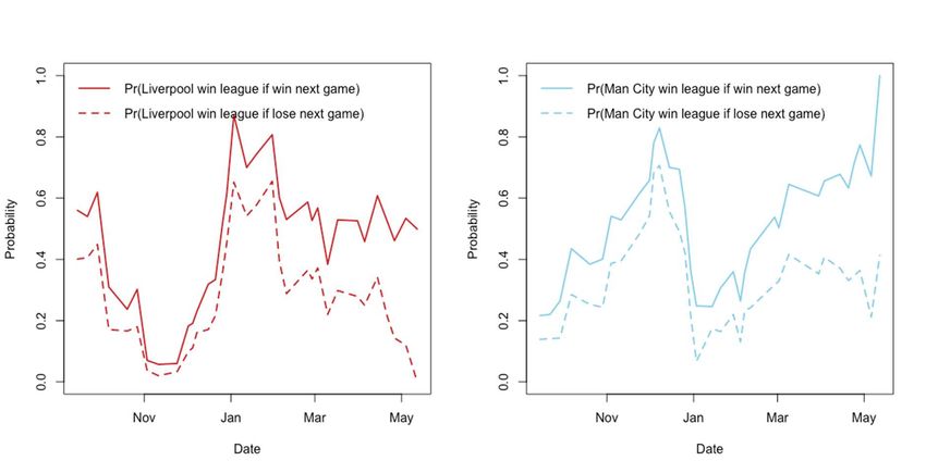
parameters). The parameters are re-estimated after each round of games, and used to simulate

the remaining matches in the season.

 The 2018-19 Premier League season saw a titanic struggle between Liverpool and the

eventual champion, Manchester City. Both clubs were able to win the championship up to the

very last game of the season. To illustrate the data generated, Figure 1 shows the probability

of each team winning the league title if it wins the next game, and if it loses the next game.

Towards the end of the season, the result of the next game has a large impact on the outcome

of the championship. Indeed, Liverpool had to win the final game to even have a chance of

winning the title. Figure 2 shows the resulting values of match significance for each team as

the season progresses. The match between the two on 3rd January 2019 is visible as a local

peak in match significance demonstrating its importance to the championship several months

before the end of the season.

 FIGURE 1
Probabilities of winning the championship conditional on the next game being won (solid line), and conditional on the next
game being lost (dashed line), for Liverpool (left), and Manchester City (right), during the 2018-19 Premier League season.

 16

FIGURE 2
 Match significance for Liverpool (red) and Manchester City (sky blue) during the 2018-19 Premier
 League season

 IV. DATA AND MODEL

A. Data

 We had access to minute-by-minute estimates of the size of the domestic audience for

every programme featuring a live EPL match between the middle of the 2013-14 season and

the end of the 2018-19 season. These were sourced from the British Audience Research

Bureau (BARB), which supplies the broadcasting and marketing industries with data on

television viewing in the United Kingdom. Its audience figures are based on a representative

panel of more than 5,000 households covering 12,000 individuals over the age of 4. As it is a

panel of households, viewing in other settings, such as bars or prisons, is not reflected in

BARB’s figures for audience size.

 17

During the period, matches were shown on either of two channels, Sky Sports and BT

Sport, each accessible to viewers by payment of a subscription.14 Sky Sports has been

supplying EPL matches to its customers since the inception of the EPL but BT Sport was in

its first season as an EPL broadcaster at the start point in our data. That season, and in each of

the following two, 154 EPL matches were televised on one or other of the channels. This

degree of exposure was increased only modestly for the final three seasons, when 168

matches were shown.

 For estimation, we discarded matches played in the first three rounds of each season

and in the last round of each season. Information from all matches in the first three weeks

was used to calibrate our match significance variables. In the last round of each season, to

assure the integrity of the competition, all matches are played simultaneously and more than

one game is shown on television. This makes conditions different from the rest of the season

when any match to be televised is scheduled to a time slot such that no other EPL fixture is

being played at the same time.15 These omissions from the data left us with 790 televised

matches to be included in regression analysis.

 For each match, we had minute-by-minute audience size data for the programme. As

noted above, programme length is highly variable and therefore our preference was to model

average per-minute audience for the match itself, which is of fixed duration, rather than for

the programme of which it is the centre-piece. Our preferred dependent variable is therefore

the natural log of the average per-minute audience size measured from kick-off to 110

minutes later. This time interval accounts for 90 minutes of regular play, 15 minutes interval

(half-time) and an assumed 5 minutes of added (injury) time. For comparison with earlier

14
 Sky subscribers can view BT matches by paying a supplementary fee.

15
 The most common time slots are lunchtime and late afternoon on Saturday and Sunday and starting around 8
p.m. on Monday.

 18

studies, we also modelled programme audience size. This is the average per-minute audience

size for the whole programme, which includes pre- and post-match content as well as the

game itself. This is the ‘headline’ statistic which will usually be quoted in the media. Its mean

across our data (829,862) was appreciably lower than the mean audience for the match itself

(1.06 millions), reflecting that pre- and post-match segments typically attract far fewer

viewers than the period of action on the field.

B. Model

 The regressors of key interest in our model are player quality, outcome uncertainty,

and three variables for match significance (representing the relevance of a match for the

championship, European qualification and relegation). Outcome uncertainty is measured as

the absolute difference in the probabilities of a win for either team, according to bookmaker

odds.16 The variables representing player quality and match significance were described in

Section III above. The expected sign on all these variables is positive.

 We also include several control variables. These include dummy variables to

represent the time of the week and the month of the year when the game was played, the

season during which it took place and the broadcaster which provided the coverage. There is

also an indicator for ‘derby match’.

 Regarding time in the week, we distinguish weekday matches (always in the evening)

from weekend matches (the reference category), in line with previous studies for the EPL. In

addition, we distinguish a third category, ‘Christmas’, which refers to the period following

Christmas Day and up to the day of the New Year Holiday (as late as January 3 in 2017,

16
 We retrieved odds offered by William Hill as displayed in the archive at football-data.co.uk. These were
expressed in decimal-odds format and the inverse of the decimal-odds gave us the ‘bookmaker-probability’ of
each outcome (home win, draw, away win). Finally, since the sum of the three bookmaker-probabilities always
exceeds 1, to allow the betting provider its commission, each bookmaker-probability was then multiplied by a
constant such that the three ‘implied probabilities’ for any match summed to 1.

 19

because the 1st had fallen on a Saturday). All matches in this period, when a large part of the

labour force is on holiday, are deemed ‘Christmas’ rather than counted as weekday or

weekend. The delineation of this third category is made because, controversially, British

leagues schedule frequent fixtures over this time rather than take a midwinter break as in

most of the rest of Europe. The alternative would be to schedule extra rounds of midweek

matches during the rest of the season and it is relevant to ask whether there is any gain if the

goal is to maximise aggregate television audience.

 Audience size is likely to depend on which broadcaster shows the match. ‘BT Sport’

is a dummy variable to distinguish its games from those covered by Sky Sports. We also

include interaction terms between BT Sport and season dummies because BT Sport was a

new entrant to the market in the first season of our data period and it would be reasonable to

suppose that its penetration of the market would be spread over time. Coefficient estimates on

the interaction terms would also reflect any differential price changes compared with the

long-time incumbent, Sky Sports. We were unable to track these though we do note that, on a

per-match basis, BT Sport subscription prices were much higher than Sky Sports, 2.6 times as

high in season 2015-16 according to Butler and Massey (2019).17

 ‘Derby match’ also features in most earlier studies. This indicator variable signals

match-ups between clubs where there is local or regional rivalry. We identified 15 such

match-ups, eight of which involved London clubs. Of the remainder, most related to clubs in

contiguous urban areas but we also included two match-ups (Liverpool- Manchester United

and Brighton-Bournemouth) where there was greater geographical separation but where

common knowledge still recognises strong rivalry. We expected that derby matches might

attract additional viewers because of extra regional interest in the relevant matches but

17
 In a private communication, Dr. Butler informed us that the differential was similar in the most recent season.

 20

possibly also on a wider geographical basis because of the perception that these games are

contested more intensely.

 Finally, and similar to, for example, Buraimo and Simmons (2015), we include a full

set of club dummies, each set equal to 1 if the relevant club was a participant in the subject

match. Some other authors, for example Pérez, Puente and Rodríguez (2017) and Forrest,

Simmons, and Buraimo (2005) were more selective in that they each included dummy

variables only for two or three clubs with national reach in support (in Spain and England

respectively). However, clubs with very different market sizes played in the EPL over our

period, including some which appeared to maintain a historically strong support base but

which were not now strong either financially or on the field. Sunderland is an example.

Representing such as Sunderland by its own dummy variable allows us to estimate the power

of club brands to draw audiences independent of the quality of their current players. The

reference club, selected on lexicographic grounds, is AFC Bournemouth, one of the smallest

market clubs in the EPL and in fact only a recent entrant to the EPL (historically, it had most

often played in the third-tier league). Because AFC Bournemouth would be the point of

reference, we anticipated that most club dummies would attract a positive coefficient

estimate.

 Our model to be estimated is:

(5) Ln (audience size) = f(player quality, outcome uncertainty, match significance

(championship), match significance (European), match significance (relegation), controls)

where controls include: club dummies, season dummies, month dummies, derby match, BT

Sport, BT Sport/season interaction terms.

 21

Because not all EPL matches are screened on television, we considered the case for

trying to account for possible selection bias when estimating this model. Two previous papers

(Forrest, Simmons, and Buraimo 2005; Buraimo and Simmons 2015) modelled broadcaster

choice of which matches to show, incorporated into a Heckman procedure. Others have

ignored the issue.18 We decided not to employ a sample selection model here, for three

reasons. First, there is no strong theoretical basis for suspecting that selected matches possess

some distinctive non-observed characteristics which would affect audience demand, given

that the set of match characteristics already included in the demand equation seems to be

rather comprehensive. Second, preceding papers which have tested for sample selection bias

have decisively rejected its presence. Third, we are not confident that we would represent the

process driving broadcaster choice accurately because they will have selected their games at

unknown dates several weeks before each round of matches takes place, so the dating of

relevant covariates would be problematic.19,20

 Tables 1a and 1b present summary statistics for variables included in the modelling.

In the data set, the match with the highest average audience (measured over the match rather

than the programme), 2.67 millions, was Chelsea v. Manchester United, played in January,

2014.

18
 It did not arise in studies for Germany and Italy, where all matches were televised.
19
 The fixtures chosen to be shown are rescheduled to the time slots designated for televised matches, for
example from Saturday afternoon to Monday evening. To allow attendees, police and ground authorities to plan,
notification must be given far in advance.

20
 Another complication of modelling broadcasters’ choice of matches to be screened is that the contracts
require them to choose four from ten pre-determined fixtures in each round. Preceding literature fails to account
for this constraint and treats the choice of matches as if it were made from all games in the season.

 22

V. FINDINGS

A. Match audience versus programme audience

 Table 2 displays results from three models, all of which were estimated with club

dummies included. The first column represents our preferred model, with the dependent

variable measuring the average audience size over the match period and the regressors

defined as above.

 It was noted earlier that results in preceding studies appear typically to have measured

average audience size over the whole programme rather than whistle-to-whistle and that this

was a risky procedure because duration of programme is highly variable. Column (2) of the

table presents estimates based on average programme rather than our preferred average match

audience size. As expected, measuring audience size over the match itself has resulted in

more precise estimation. The standard deviation of the match audience variable (468,241) is

larger than the standard deviation of the programme audience variable (380,248) but still the

 TABLE 1a
 Summary Statistics for Continuous Variables, N=790
 mean std. dev. min max
 programme audience 829,682 380,248 171,500 2,432,500
 match audience 1,062,880 468,241 181,199 2,672,705
 average player rating 0.013 0.012 -0.020 0.047
 combined relative wages 2.410 0.767 0.872 4.470
 outcome uncertainty 0.341 0.217 0.000 0.885
 match significance (championship) 0.063 0.101 0.000 0.995
 match significance (European) 0.136 0.133 0.000 0.920
 match significance (relegation) 0.088 0.125 0.000 1.597

 23

TABLE 1b
 Summary Statistics for Discrete Variables, N=790
 mean std. dev.
derby match 0.116 0.321
Christmas 0.060 0.237
weekday 0.213 0.409
October 0.095 0.293
November 0.094 0.292
December 0.148 0.355
January 0.111 0.315
February 0.108 0.310
March 0.108 0.310
April 0.163 0.370
May 0.086 0.281
BT 0.257 0.437
BT × season ending: 2015 0.044 0.206
BT × season ending: 2016 0.043 0.203
BT × season ending: 2017 0.049 0.217
BT × season ending: 2018 0.049 0.217
BT × season ending: 2019 0.048 0.214
season ending: 2015 0.172 0.378
season ending: 2016 0.171 0.377
season ending: 2017 0.189 0.391
season ending: 2018 0.190 0.392
season ending: 2019 0.187 0.390

 24

TABLE 2

 Regression results: dependent variable is Ln(audience)
 (1) (2) (3)
 match audience programme audience match audience
 coeff. |t| coeff. |t| coeff. |t|
 average player rating 3.974*** (2.92) 4.059*** (2.95)
 combined relative wages 0.040 (0.71)
 outcome uncertainty -0.037 (0.80) -0.010 (0.21) -0.031 (0.67)
 derby match 0.050* (1.83) 0.050 (1.61) 0.051* (1.83)
 match significance (championship) 0.675*** (5.21) 0.576*** (4.49) 0.788*** (6.18)
 match significance (European) 0.205* (1.94) 0.173* (1.71) 0.226** (2.13)
 match significance (relegation) 0.341*** (3.89) 0.344*** (3.39) 0.274*** (3.05)
 Christmas 0.100*** (2.86) 0.146*** (3.70) 0.093*** (2.70)
 weekday 0.016 (0.80) -0.129*** (6.34) 0.015 (0.75)
 October 0.017 (0.46) 0.027 (0.64) 0.018 (0.47)
 November 0.106*** (3.06) 0.128*** (3.22) 0.106*** (3.01)
 December 0.121*** (3.58) 0.146*** (3.79) 0.120*** (3.55)
 January 0.196*** (5.63) 0.228*** (6.06) 0.196*** (5.58)
 February 0.119*** (3.59) 0.161*** (4.38) 0.117*** (3.52)
 March 0.053 (1.42) 0.102** (2.48) 0.053 (1.39)
 April 0.047 (1.48) 0.094*** (2.70) 0.043 (1.32)
 May -0.141*** (2.67) -0.055 (1.10) -.149*** (2.83)
 BT -0.781*** (16.12) -0.859*** (14.92) -.779*** (15.97)
 BT × season ending: 2015 0.131** (2.22) 0.207*** (2.94) 0.125** (2.09)
 BT × season ending: 2016 0.253*** (4.08) 0.283*** (3.93) 0.239*** (3.75)
 BT × season ending: 2017 0.305*** (4.93) 0.354*** (5.06) 0.299*** (4.83)
 BT × season ending: 2018 0.378*** (5.87) 0.427*** (5.86) 0.375*** (5.75)
 BT × season ending: 2019 0.278*** (4.37) 0.351*** (4.94) 0.280*** (4.39)
 season ending: 2015 -0.090** (2.30) -0.138*** (3.10) -0.084** (2.19)
 season ending: 2016 -0.170*** (4.09) -0.176*** (3.97) -.170*** (4.18)
 season ending: 2017 -0.295*** (7.50) -0.285*** (6.52) -.298*** (7.80)
 season ending: 2018 -0.292*** (6.89) -0.297*** (6.30) -.288*** (6.95)
 season ending: 2019 -0.218*** (5.04) -0.228*** (4.81) -.236*** (5.54)
 constant 13.416** (156.93) 13.154** (140.43) 13.375** (123.53)
 observations 790 790 790
 adj-R2 0.717 0.705 0.714
 aic 32.936 114.338 42.544
 root MSE 0.239 0.251 0.240
 Absolute t statistics in parentheses
 *
 p < 0.1, ** p < 0.05, *** p < 0.01

root mean square error of the match audience equation is appreciably lower. This encourages

us to believe that modelling based on the audience just for the match itself should allow more

reliable inference concerning the preferences of viewers. Differences in substantive findings

on focus variables are limited; but modelling match audience does sharpen coefficient

estimates on the match significance variables, and in particular allows reasonable inference to

be drawn that there is some attraction to matches significant for European qualification. This

would not be possible from the estimated programme audience equation. Among control

variables, the coefficient estimate on ‘weekday’ changes from significantly negative in the

programme audience equation to essentially zero in the match audience equation. This might

 25

be considered surprising because the mean duration of both pre- and post-match content is

more than twice as long for weekend than for weekday matches. Thus programme audience

data at the weekend should be pulled down to a greater extent than midweek through being

diluted by non-match content. However, the result we obtained implies that there is much less

propensity for audience members to view pre- and post-match content on a weekday evening.

This is plausible given that, for many, the pre- and post-match periods come soon after work

and before bedtime respectively. For the match itself, viewership does not seem to vary

between the weekend and a weekday evening.

B. Player quality

 Our measure of quality, which is average player rating across the two starting elevens,

is strongly significant as a predictor of audience size. The effect size is modest (relative to the

influence of club brands, to be discussed below) but far from trivial. A match featuring a

group of 22 starting players which had an average player rating one standard deviation above

rather than one standard deviation below the mean would increase expected audience size by

about 11%. 21, 22

 We reviewed whether the use of our metric for player quality had made a material

difference to findings. In three preceding studies of television demand for EPL football

(Forrest, Simmons, and Buraimo 2005; Buraimo and Simmons 2015; Scelles 2017), the

21
 In unreported experimentation, we tested for superstar effects by including an additional variable, the rating of
the highest rated player. This variable proved decisively non-significant and its presence made minimal
difference to other covariate estimates.
22
 Buraimo and Simmons (2015) also report that player quality matters and draw the policy implication that
restrictions on player recruitment might be damaging. That issue is even more relevant now when immigration
restrictions following the United Kingdom’s withdrawal from the European Union threaten free movement of
labour. On the other hand, Buraimo and Simmons may have been too hasty to draw their conclusion. Results
where the player quality measure is significant demonstrate that British viewers are selective over which
matches to view. The data cannot show how their behaviour might change if the average talent level in the
League were lowered uniformly. One cannot rule out that they would continue to watch the same number of
matches and continue to choose amongst them according to relative talent levels across matches.

 26

alternative metric of ‘combined relative wages’ of the two clubs had been employed and this

metric also featured in analysis of the Italian League by Caruso, Addesa, and Di Domizio

(2019). Table 2, column 3, shows results from estimating our preferred model with combined

relative wages substituted for average player rating. Had we been content with this variable,

we would have concluded that viewers were unresponsive to player quality. Our assessment

of the effect sizes from the match significance variables would also have been different. So

introduction of our metric, rooted in sport analytics, did indeed change findings in a

substantive way.

 Nevertheless, for all its imperfection, we were curious as to the complete failure of the

combined relative wages variable to account for variation in audience size. It is plausible that

the measure is at least positively correlated with whatever is meant by player ability23 and the

preceding studies found a role for it in their modelling (for earlier periods than ours). In

unreported regression, we re-estimated with combined relative wages as the player quality

variable but with club dummies omitted. Now the combined relative wages measure was

strongly significant. So it appears to be standing as a proxy for club dummies. Our

interpretation is that, over the data period we analyse, there was such stability across seasons

in the distribution of clubs’ relative spending on wages that the information in the wages

measure will have been collected in the coefficient estimates on the club dummies in our

preferred equation. Recall that a weakness of the wages measure is that it is invariant

whenever in the season a particular match occurs. The advantage of the player ratings

measure is that it can exploit information readily available to fans concerning the actual

ability of the players currently available to play and evolves over time. For example, it can

represent a situation where a club has struck unusually well- or unusually ill-judged contracts

23
 In our data set, the correlation coefficient between average player rating and combined relative wages was
+.655.

 27

with new players such that actual rather than (wrongly) assumed player ability is measured.

Likewise it can reflect information about changed personnel during a season, such as when a

club has hired or sold important players or when a key player is lost to long-term injury. The

additional variability allows viewer preferences for quality to be teased out and separated

from the popularity of clubs. We therefore recommend that a metric of this type should be

employed in future research.

C. Outcome uncertainty

 Our outcome uncertainty measure, based on outcome probabilities from the betting

market, was decisively non-significant. In case this finding concealed non-linear preferences,

we experimented also with using a spline for outcome uncertainty but could identify no part

of the range of the outcome uncertainty variable where the relationship between audience size

and the value of the variable had a non-zero slope. Our result is therefore inconsistent with

the uncertainty of outcome hypothesis.

 We are far from alone in failing to uncover evidence that, in competitions as currently

constituted, viewers’ decisions are influenced by how well-balanced a particular fixture is.

Reviewing the relevant literature, Budzinski and Pawlowski (2017) noted that television

demand studies in sport “struggle in providing clear evidence for the importance of short-

term uncertainty across settings”. Their review suggests that the same is true in the context of

stadium attendance research.

 There is some previous work on television demand which does claim support for the

uncertainty of outcome hypothesis. However, we are sceptical over whether that is what the

relevant papers in fact established. Cox (2018) represents outcome uncertainty by including

seven bands of ‘home win probability’ (as implied by bookmaker odds), using the band 5.9%

to 17.6% as reference. The paper reports that the coefficient estimate on the band 35.9% to

 28

45% was statistically significant (though none of the other bands had a significant impact).

Now it is true that a home win probability around 40% would (once the draw probability was

accounted for) indicate a finely balanced match. However, the results table indicates

significance only at the 10% level. Further, in an alternative specification, the paper enters

home win probability as a quadratic and neither component is significant even at 10%

(whereas the uncertainty of outcome hypothesis would predict an inverted-U shape). While

the paper claims to provide support for the uncertainty of outcome hypothesis, our reading of

it is that the evidence offered points in the other direction.

 Other authors have investigated whether consumers’ tastes for uncertainty of outcome

may have varied over time. Buraimo and Simmons (2015) and Schreyer, Schmidt, and

Torgler (2016) interacted uncertainty of outcome (derived from bookmaker odds) with season

dummies. The first paper, which was on EPL viewing figures, reported that the outcome

uncertainty variable itself, the gap between the clubs’ win probabilities, was non-significant

but that the first two of the eight interaction terms were negative and significant (at 10%).

The authors suggested that this pattern of results, significance in the first two years only, may

have reflected an evolution of viewer preferences away from a focus on outcome uncertainty.

However, they ignored the multiplicity issue. They carried out eight tests on interaction terms

and two of the terms were significant at 10%. With an appropriate adjustment in the p-value

required to reject the null hypothesis, to account for multiplicity, all the interaction terms, as

well as the outcome uncertainty variable itself, would have been non-significant at 10%. Our

interpretation of their evidence is therefore that there was no support in their data for the idea

that viewers were responsive to uncertainty at any point in their data period. Their results are

therefore consistent with ours (from a data period which is non-overlapping with ours).

 In their study of German league football, Schreyer, Schmidt, and Torgler (2016) also

claimed to detect changing preferences, according to coefficient estimates on their interaction

 29