UNIFYING CARDIOVASCULAR MODELLING WITH DEEP REINFORCEMENT LEARNING FOR UNCERTAINTY AWARE CONTROL OF SEPSIS TREATMENT - arXiv.org
←
→
Page content transcription
If your browser does not render page correctly, please read the page content below
U NIFYING C ARDIOVASCULAR M ODELLING WITH D EEP
                                              R EINFORCEMENT L EARNING FOR U NCERTAINTY AWARE
                                                         C ONTROL OF S EPSIS T REATMENT

                                                                                       Thesath Nanayakkara
                                                                                     Department of Mathematics
arXiv:2101.08477v2 [cs.LG] 2 Feb 2021

                                                                                      University of Pittsburgh
                                                                                       Pittsburgh, PA, 15213

                                                                                            Gilles Clermont
                                                                                Department of Critical Care Medicine
                                                    The Clinical Research, Investigation, and Systems Modeling of Acute Illness (CRISMA) Center
                                                                             University of Pittsburgh School of Medicine
                                                                                         Pittsburgh, PA, 15213

                                                     Christopher James Langmead                                   David Swigon
                                                    Computational Biology Department                      Department of Mathematics
                                                      School of Computer Science                    McGowan Institute for Regenerative Medicine
                                                       Carnegie Mellon University                           University of Pittsburgh
                                                         Pittsburgh, PA, 15213                               Pittsburgh, PA, 15213

                                                                                            A BSTRACT
                                                Sepsis is the leading cause of mortality in the ICU, responsible for 6% of all hospitalizations and
                                                35% of all in-hospital deaths in USA [1]. However, there is no universally agreed upon strategy for
                                                vasopressor and fluid administration [2]. It has also been observed that different patients respond
                                                differently to treatment [3], [4], highlighting the need for individualized treatment.
                                                Vasopressors and fluids are administrated with specific effects to cardiovascular physiology in
                                                mind and medical research has suggested that physiologic, hemodynamically guided, approaches to
                                                treatment is prudent [5]. Thus we propose a novel approach, exploiting and unifying complementary
                                                strengths of Mathematical Modelling, Deep Learning, Reinforcement Learning and Uncertainty
                                                Quantification, to learn individualized, safe, and uncertainty aware treatment strategies.
                                                We first infer patient-specific, dynamic cardiovascular states using a novel physiology-driven recurrent
                                                neural network trained in an unsupervised manner. This information, along with a learned low-
                                                dimensional representation of the patient’s lab history and observable data, is then used to derive
                                                value distributions using Batch Distributional Reinforcement Learning.
                                                Moreover in a safety critical domain it is essential to know what our agent does and does not know, for
                                                this we also quantify the model uncertainty associated with each patient state and action, and propose
                                                a general framework for uncertainty aware, interpretable treatment policies. This framework can be
                                                tweaked easily, to reflect a clinician’s own confidence of the framework, and can be easily modified
                                                to factor in human expert opinion, whenever it’s accessible. Using representative patients and a
                                                validation cohort, we show that our method has learned physiologically interpretable generalizable
                                                policies.
                                                We posit that this work takes an important step towards a safe, physiology and uncertainty aware, deci-
                                                sion support system for septic patients. It also provides a general framework for using Reinforcement
                                                Learning to support healthcare applications involving sequential decisions.
                                                1

                                        1
                                            Code for this work can be found at //github.com/thxsxth/POMDP_RLSepsis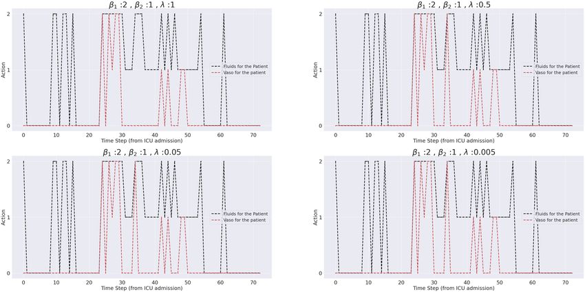
A PREPRINT

1       Introduction

Sepsis is an overwhelming and extreme response to infection which can result in tissue damage, organ damage and
death. Sepsis has been described as the leading cause of mortality in U.S. hospitals [6]. Moreover sepsis has been
attributed to approximately 6 % of all hospitalizations and 35% of all in-hospital deaths in U.S [1].
Reinforcement Learning (RL) [7] is a sub-field of machine learning and control engineering dealing with sequential
decision making problems. RL, especially when used in conjunction with deep neural network-based function
approximation (Deep Reinforcement Learning/DRL) has achieved super-human performance in various domains [8]
[9], [10]. It also has many desirable properties for healthcare problems, including applications to personalized medicine
[11], [12]. But there remains considerable challenges in applications to practical medical decision making.
Herein, we identify major challenges in applying RL algorithms directly to find optimal treatment for sepsis and
leverage distinct strengths of mechanistic physiological models, deep learning and RL to propose an uncertainty aware,
RL based decision support system, which addresses each of the challenges.
Consistent with previous work [13], [14], [15], we focus on vasopressor and IV fluid treatments, which whilst regarded
important, studies have shown significant variation among patient responses to them [3],[4] [16]. Further there is little
agreement among medical researchers on best practices that guide fluid or vasopressor administration beyond initial
resuscitation. Both have been shown to be associated with negative effects on some patients. [17]
Vasopressors and fluids are intended to counteract hypovolemia (abnormally low extracellular fluid), sepsis induced
vasodilation (dilatation of blood vessels) vasoplegia (decreased response to compensatory mechanisms that increase
vascular tone in normal physiological states) and physiological disturbances observed in sepsis. For instance it has been
observed that vasodilatation of systemic resistance vessels in severe sepsis can decrease by up to 75% [18]. Recent
recommendations [5] have argued for a hemodynamically-guided fluid resuscitation strategies for patients with severe
sepsis and septic shock.
Therefore it is clear that accurate cardiovascular states should provide crucial information for deciding on proper
treatment. For this purpose we introduce a novel inference structure which is in essence a denoising recurrent
autoencoder [19], implicitly regularized by constraining the decoder to be a physiologic cardiovascular model. This
dynamically learns a patient specific, robust cardiovascular state representation, in an unsupervised manner.
Although Deep Reinforcement Learning (DRL) has achieved super-human performance in the online setting (where the
agent could interact with the environment and collect more data whilst learning), our problem belongs to the subset of
Batch Reinforcement Learning [20] (Batch RL), where we do not have access to the real-time environment and all the
learning is carried out using a retrospective fixed dataset. It is also well known that DRL could perform quite poorly
when it is trained using a fixed dataset, and that its generalizability depends on the training data used [21]. Deep neural
networks in general also have the tendency to yield unreliable and sometimes blatantly wrong results for data far from
the training distribution. Therefore, we claim that it is essential to address model uncertainty and quantify what the
model does know and what it doesn’t. For this purpose we propose a method to quantify model uncertainty 2 , and we
then use this to propose uncertainty aware treatment strategies, which are more suited for safety critical domains such
as healthcare.
In summary, we identify three significant challenges in directly applying DRL to compute optimal, personalized
treatment strategies.

         • Partial Observability : Vasopressor and fluid therapy are administrated with specific cardiovascular goals in
           mind, however cardiovascular states cannot be observed, and despite the richness of data collected in the ICU,
           the mapping between patient states and clinical observables is often ambiguous, arguably a major contributor
           to variation in clinical practice.
         • Model Uncertainty : Deep neural networks are usually used as black box models and the learning of function
           approximating networks is dependent on the training data. Thus, in situations where the extent and the variety
           of the training data cannot possibly cover the feasible range of situations (physiologic states and actions), as is
           the case in complex clinical situations such as sepsis, it is critical to quantify what the model does not know.
         • Problems associated with Batch RL : When the learning is done using a fixed retrospective dataset, it has
           been shown that the learned policies could be sub-optimal [21].
    2
     Here, and throughout this work we use the term ’model uncertainty’ to mean the uncertainty associated with neural networks
used for RL. This should be not be confused with the model-based vs model-free RL distinction, because (once we have inferred
latent states), our approach qualifies as ’model-free’. Uncertainty Quantification literature also uses the term epistemic uncertainty
for model uncertainty

                                                                  2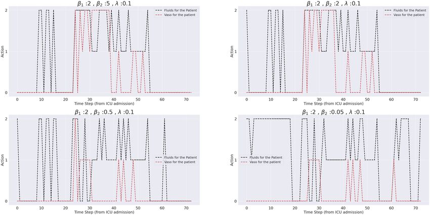
A PREPRINT

Our work extends previous work in applying DRL for sepsis treatment, addressing each of the challenges above.

       • Partial Observability : We propose a general approach to combine physiologic modelling with deep networks
         to learn patient specific physiological states in an unsupervised manner, and use this framework to infer
         cardiovascular states of ICU patients. We further encode the entire patient laboratory history using a denoising,
         stacked, recurrent autoencoder architecture. This representation learning is expected to provide valuable
         hidden information to further characterize states which can be exploited by our agent.
       • Model Uncertainty Quantification : We associate an uncertainty measure for each state-action pair, which
         quantifies model uncertainty and the randomness introduced by training process.
       • Problems Associated with Batch RL : We use a distributional approach to RL. This approach has been
         shown to achieve superior performance in Batch RL [22]. Poor results in Batch RL is usually attributed to
         the fact that some state-action pairs are sparsely represented in the training dataset. To counter this, we use a
         discrete set of actions, all of which are observed frequently in the training dataset.

2     Background

2.1   Reinforcement Learning

Reinforcement Learning [7] is a general framework for optimizing sequential decision making. In its standard form, a
(discounted) Markov Decision Process (MDP), consisting of a 5-tuple (S,A,r,γ,p) is the framework considered. Where
S and A are state and action spaces. r : (S, A, S) → R is a (possibly stochastic) reward function, p : (S, A, S) → [0, ∞)
denotes the unknown environment dynamics, which specifies the distribution of the next state s0 , given the state-action
pair s, a and γ is a discount rate applied to rewards.
In the partially observed setting there is a distinction between the observations, usually denoted as ot , and the true
state st , and the environment dynamics include the conditional probability density p(ot |st ). This yields the probability
density of a particular observation, given the true underlying state. This extends the MDP formalism to that of Partially
Observed Markov Decision Process (POMDP).
A policy is (a possibly stochastic) mapping from S to A.
The agent aims to compute the policy π which maximizes the expected future reward Ep,π [Σt γ t rt ], where the expected
value is with respect to the policy π and the unknown environment dynamics p.
The value V π for a state s, is defined to be the expected future discounted rewards, by following policy π, starting from
the state S.

                                         V π (s) = Ep,π [Σt rt (st , at )|s0 = s, π]                                   (1)

The Q function is the expected future reward resulting from choosing action a, and then continuing the policy π.

                                   Qπ (s, a) = Ep,π [Σt rt (st , at )|s0 = s, π, a0 = a]                               (2)

Central to most value-based RL algorithms is the Bellman equation [23],

                                      Qπ (s, a) = Ep [r(s, a)] + γEp,π [Qπ (s0 , a0 )]                                 (3)

and the Bellman optimality equation,

                                  Q∗ (s, a) = Ep [r(s, a)] + γEp [maxa0 ∈A Q∗ (s0 , a0 )]                              (4)
(where Q∗ (s, a) is the optimal Q function, and s0 denotes the the random next state)
Most modern DRL algorithms use parameterized neural network function approximators, to approximate the Q function,
and learn using 3 or 4 as a loss function.

                                                             3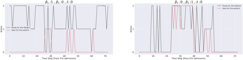
A PREPRINT

                                                                                                    a

                                                                       b                                           c
Figure 1: a : Proposed decision making process : We use the compete patient history, which includes, vitals, scores, and labs, and
previous treatment, to infer hidden states. These would all combine to make the state St . Our trained agent, takes this state and
outputs value distributions for each treatment, it’s own uncertainty, and an approximate clinician’s policy. We then factor in all 3 to
propose uncertainty-aware treatment strategies. b :Complete physiology-driven autoencoder network structure Patient history is
sequentially encoded using three neural networks. A patient encoder computes initial cardiovascular state estimates using patient
characteristics, a recurrent neural network (RNN) encodes the past history of vitals and scores, up to and including the current time
point, and a transition network which takes the previous cardiovascular state, the action and the history representation to output new
cardiovascular state estimates. c :The electrical analog of the cardiovascular model This provides a lumped representation of the
resistive and elastic properties of the entire arterial circulation using just two elements, a resistance R and a capacitance C. This
model is used to derive algebraic equations relating R, C, stroke volume (SV), filling time (T), to heart rate (F) and pressures. These
equations define the decoder of the physiology-driven autoencoder.

Distributional Reinforcement Learning Distributional Reinforcement Learning [24][25][26], tries to learn (an
approximation of) the entire return distribution associated with a state-action pair. It has been shown [22] that
distributional reinforcement learning has achieved superior performance in Batch Reinforcement Learning.
More formally, the return associated with a policy π now is considered as a random variable Z π (s, a), and the Q
function is the expectation of Z. Following the notation from [24], the distributional Bellman equation can be written
down as,

                                                Z(s, a) =d R(s, a) + γZ(S 0 , A0 )                                                 (5)

                                                                  4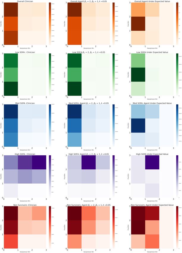
A PREPRINT

Where =d indicates distributional equivalence, (S 0 , A0 ) is a random variable tuple representing the next state, action.
We use the categorical distributional reinforcement learning algorithm, proposed by [24], where the value distribution is
approximated by a discrete distribution with equally spaced support.

Imitation Learning Unlike in Reinforcement Learning where the agent tries to find the optimal policy, in Imitation
Learning the goal is to successfully imitate an expert.
We use Imitation Learning (more specifically behavior cloning) to learn a clinician policy which is then used, when
recommending an action. Further details of this are included under methods. (section 4.5)

2.2   Unsupervised Representation Learning

Representation learning is described as learning representations of the data that make it easier to extract useful
information. [27]. Most of the success of modern machine learning and neural networks can be attributed learning
effective representations of data. One common way of learning useful representations is to use outputs of hidden layers
of a neural network trained for one, possibly easy, auxiliary task for another task. This is the path we follow, when we
encode the entire lab history of a patient, using a denoising autoencoder. Our physiology-driven autoencoder is itself a
representation learner. However the representations have physiological meanings.
We argue that in Batch RL, where obtaining new data is impossible, learning useful representations can be the key to
learning effective and generalizable RL policies.

2.3   Uncertainty Quantification

Uncertainty Quantification (UQ) [28] is omnipresent in computational sciences, applied mathematics, engineering and
machine learning. As the name suggests, UQ is the science and methods of identifying and quantifying uncertainty in
wide range of computational, statistical and engineering domains.
Uncertainty is usually categorized into two categories: aleatoric uncertainty, the inherent randomness in the environment,
and epistemic or model uncertainty, which reflects how uncertain a model is of its own results. It is the later that we
will be focusing on this work.

3     Related Work
Reinforcement Learning for Sepsis treatment : RL has been used for various healthcare applications. [12] and
[11] provide comprehensive surveys of these applications of RL in healthcare and critical care applications respectively.
Regarding using vasopressor and intravenous fluids for treatment of sepsis, Komorowski et al. [13] used a discrete
state representation created by clustering patient physiological readouts, and a 25 dimensional discrete action space to
compute optimal treatment strategies using dynamic programming based methods. This work was both confirmed and
criticized (e.g. Jeter [29]). This approach was extended by the authors to alternative reward schemes more in line with
current medical decision making, and continuous state spaces. Raghu et al. [14] used DRL (with a Dueling DDQN [30]
algorithm) and a continuous state representation. Peng et al. [15] considers partial observability. This approach learns a
representation of the patient history using a recurrent autoencoder, and uses a mixture of experts approach combing
kernel based RL, and Deep RL. The idea presented here, of combining two different policies, has some similarities with
the framework we introduce in section 4.5 to factor in human behavior likelihood and uncertainty. Recent work [31]
has focused on considering partial observability and continuous action.

Uncertainty aware Reinforcement Learning : Various UQ methods to identify, quantify and sometimes reduce,
uncertainty in machine learning have been proposed in recent years. Abdar et al [32] reviews these methods and
investigates their applications. Most of these methods use one or more of Bayesian Neural Networks (BNN), Concrete
Dropout (CD), and Deep Ensembles (DE) [33].
In RL, model uncertainty has been considered previously for various safety critical learning tasks. Kahn et al. considers
uncertainty aware navigation of mobile robots [34]. They use a model-based RL algorithm based on a predictive model
comprising of bootstrapped neural networks using dropout. Lotjens et al. [35] uses an ensemble of collision prediction
networks, bootstrapping and Monte-Carlo Dropout to provide uncertainty estimates for safe RL for pedestrian collision
avoidance. Bootstrapping and Deep Q Learning were also used in combination towards efficient exploration in online
learning [36]. These authors suggest an ensemble of Q networks, which then approximate a distribution over the Q
values.

                                                            5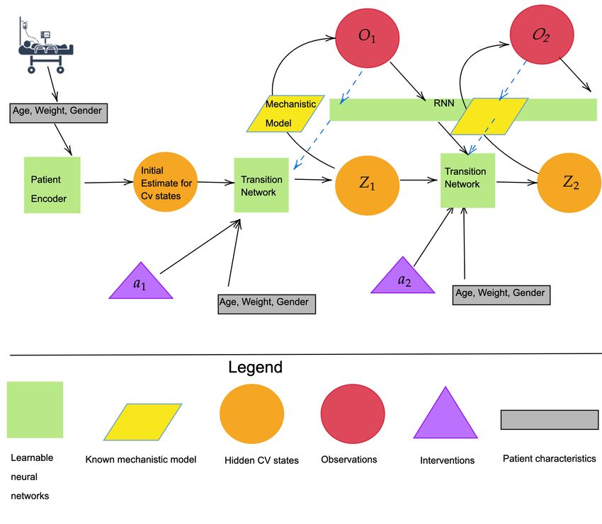
A PREPRINT

Our approach belongs to the class of Deep Ensembles and is similar to previous work in computational aspects. Yet,
we aim to answer a slightly different question. As we are interested in Batch RL, we wish to capture the uncertainty
resulting from using a limited, fixed subset of the data distribution, the stochastic gradient based learning process, and
uncertainty of the output of the neural networks.
Thus we approach the problem from a pure uncertainty quantification point of view. We do not change the training
algorithm. Rather, we formalize the concept of a state, action conditioned uncertainty associated with our problem and
Batch RL in general. We then carry out an uncertainty quantification step which computes a Monte-Carlo estimate of
uncertainty using bootstrapping. This is explained in more detail under methods.(section 4.4)

Cardiovascular Modelling : There is a vast amount of rich literature, on mathematical models being used to model
cardiovascular physiology. The mechanistic model we use (explained in detail under methods) is used in [37], and [38]
amongst other work. The overall idea of combining mechanistic models with neural networks was partially inspired by
clinical bias and a recent manuscript by Raissi et al. titled "Physics informed neural networks" [39], Which uses deep
networks to solve forward and inverse problems involving nonlinear partial differential equations.

4         Methods
4.1       Data sources and preprocessing

Our cohort consisted of adult patients (≥ 17) who satisfied the Sepsis 3 [40] criteria from the Multi-parameter Intelligent
Monitoring in Intensive Care (MIMIC-III v1.4) database [41], [42]. We excluded patients with more than 25 % missing
values after creating hourly trajectories, and patients with no weight measurements recorded. Our starting point of
trajectories is ICU admission.
We further excluded patients who got discharged from the ICU but ended up dying a few days or weeks later at the
hospital as we don’t have access to their patient data after the ICU release, and treating the final ICU data as a terminal
state would damage generalizability.
Actions were selected by considering hourly total volume of fluids (adjusted for tonicity), and norepinephrine equivalent
hourly dose (mcg/kg) for vasopressors. In computing the equivalent rates of each treatment, we followed the exact same
queries as Komorowski et al [13]. When different fluids were administrated, we summed up the total fluid intake within
the hour, and discretized the resulting distribution. For vasopressors, we considered the maximum norepinephrine
equivalent rate administrated within the hour to infer the hourly dose. We used 0.15 mcg/kg/min norepinephrine
equivalent rate, and 500 ml for fluids, as the 1,2 cutoff when discretizing.3 . A separate 0 action for each was added to
denote no treatment.
Missing vitals and lab values were imputed using a last value carried forward scheme, as long as missingness remained
less than 25% of values. A detailed description on extracting, cleaning and implementation specific processing as well
as additional cohort details are included in the appendices.

4.2       Models

4.2.1      Physiology-driven Autoencoder
Autoencoders are a type of neural networks which learn a useful latent, typically lower-dimensional representation of
input data, while assessing the fidelity of this representation by minimizing data reconstruction error. Our autoencoder
architecture provides an implicit regularization by constraining the latent states to have physiological meaning, and the
decoder to be a fixed physiologic model described in the next section. We further use a denoising scheme by randomly
zeroing out input with a probability of 10-25% , when feeding into the network. This random corruption forces the
network to take the whole patient trajectory (prior to the current time point) and previous treatment into account when
producing its output, because it prevents the network from memorizing the current observation. In essence, we ask the
inference network to predict observable blood pressures and the heart rate using corrupted versions of itself, by first
projecting it into the cardiovascular latent state, and then decoding that to reconstruct.
Figure 1 (b), shows the complete architecture of our inference network. As shown in the figure, the encoder is comprised
of three neural networks, a patient encoder which computes initial hidden state estimates, a Gated recurrent Unit (GRU)
[43] based recurrent neural network to encode the past history of vitals and scores up to and including the current time
point, and a transition network which takes the previous state, the action and the history representation to output new
      3
    These were chosen, considering the mean, median of non zero rates and medical knowledge, We also observe that due to the low
dimensional action space, there is flexibility in choosing the cutoffs

                                                               6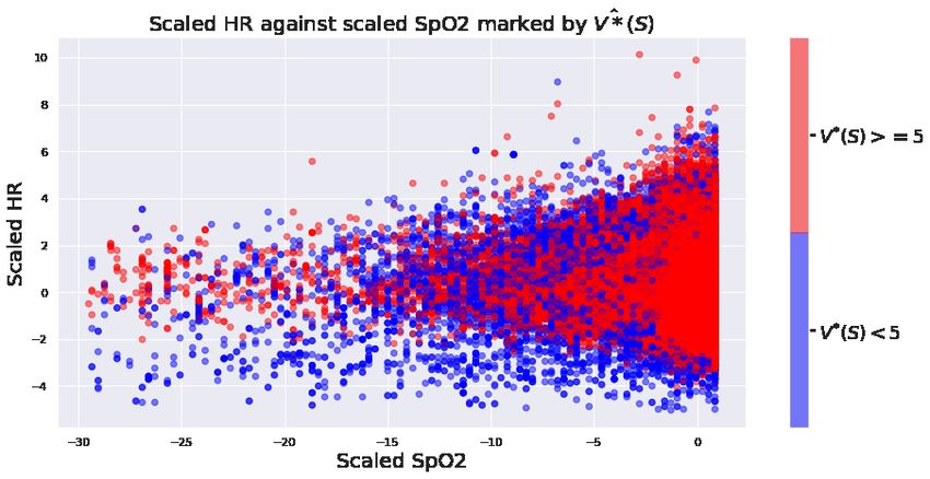
A PREPRINT

cardiovascular state estimates. We train this structure end-to-end by minimizing the reconstruction loss, using stochastic
gradient-based optimization. Appendices provide a detailed description of model and architecture hyper-parameters,
and training details.

Cardiovascular Model The cardiovascular model, is based on a two-element Windkessel model illustrated using the
electrical analog in Figure 1 (c). This model provides a lumped representation of the resistive and elastic properties of
the entire arterial circulation using just two elements, a resistance R and a capacitance C, which represent the systemic
vascular resistance (SVR), and the elastance properties of the entire systemic circulation. Despite it’s simplicity, this
model has been previously used to predict hemodynamic responses to vasopressors [38] and as an estimator of cardiac
output and SVR [37].
The differential equation representing this model is:
                                              dP (t)     1         Q(t)
                                                     =−    P (t) +                                                       (6)
                                               dt       RC          C
were Q(t) represents the volume of blood in the arterial system. As explained in [38], over the interval [0, T ] (where T
is the filling time of the arterial system) we can write Q(t) as Q(t) = SV δ(t), where SV stands for Stroke Volume, the
volume of blood ejected from the heart in a heartbeat. When the system is integrated over the interval [0, T ] we obtain
the following expressions for Psys ; Pdias ; PM AP , i.e., the systolic,diastolic, mean arterial pressures, respectively,

                       SV      1                       SV e−T /RC                       (SV )R   (SV )F R
              Psys =                  ,      Pdias =                  ,      PM AP =           =                         (7)
                        C 1 − e−T /RC                   C 1 − e−T /RC                     T         60
T is the filling time and F is the heart rate, which is determined by T . This system of algebraic equations is used for
the decoder of our autoencoder. Since heart rate can itself be affected by vasopressors and fluids, we added heart rate
(F ) as an additional cardiovascular state despite it being observable.
Therefore we have a multivariate function f : {R, C, SV, F, T } → {Psys , Pdias , PM AP , F }, represented by the
equations above, and the trivial relationship F = F (Despite the obvious relationship we used both F and T , for
ease of training and stability.) As stated previously, to prevent it from just using the current observations, we use a
denoising scheme for training. This ensures at a fixed time, the model cannot memorize the current observation and
learn to invert f , since there is a nonzero probability of corruption. Thus it has to learn to factor in the history and the
treatments when determining the cardiovascular states. Once SV is inferred, the cardiac output (CO), can be computed
as CO = (SV )F .
Since f is not one to one, typically not all states are identifiable. To arrive at a better approximation we used the latent
space to only model deviations from fixed baselines. We also posit that identifiable combinations of states when trained
with a denoising scheme should provide important cardiovascular representations in the POMDP setting.

4.2.2   Denoising GRU autoencoder for representing Lab history
We use another recurrent autoencoder to represent patient lab history, motivated by the fact that labs are recorded only
once every 12 hours. Forward filling the same observation for 12 time points, is more than likely sub-optimal, and the
patterns of change in lab history can be helpful in learning a more faithful representation. Thus we use a denoising
GRU autoencoder constructed by stacking three multi-layer GRU networks on top of each other, with a decreasing
number of nodes in each layer, the last 10 dimensional hidden layer was used as our representation. This architecture is
motivated by architectures used in speech recognition [44].
This model was also trained by corrupting the input, where each data-point was zeroed with a probability of up to 50%.
(The rate was gradually increased from 0 to 50%). As with the previous autoencoder, this provides an extra form of
regularization, and forces the learned representation to encode the entire history.
Model architecture and training details and presented in the appendix.

4.2.3   Imitation Learner
We use a standard multi-layer neural network as our imitation learner. This model is trained using stochastic gradient-
based optimization by minimizing the negative log-likelihood loss, between the predicted action and the observed
clinician action, with added regularization to prevent overfitting.
We do mention that there are many other options that could be used as a imitation learner, including nearest neighbor-
based method as in [15].

                                                             7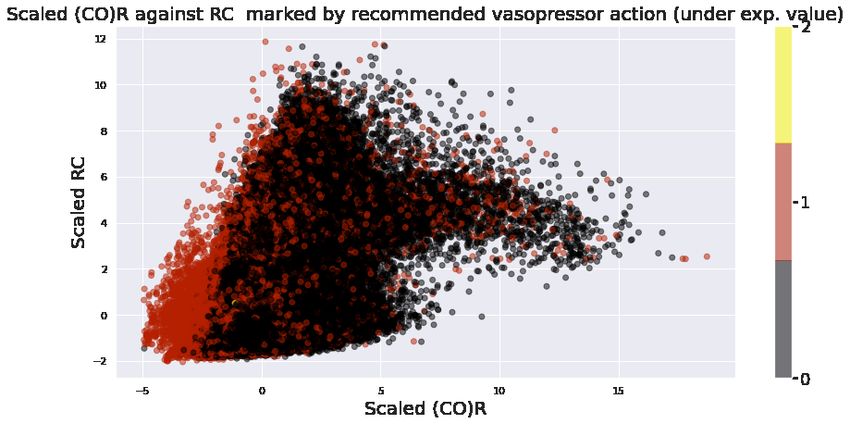
A PREPRINT

4.3     POMDP Formulation

States: A state is represented by 41 dimensional real-valued vector.

         • Demographics: Age, Gender, Weight.
         • Vitals: Heart Rate, Systolic Blood Pressure, Diastolic Blood Pressure, Mean Arterial Blood Pressure, Temper-
           ature, SpO2, Respiratory Rate.
         • Scores: 24 hour based scores of, SOFA, Liver, Renal, CNS, Cardiovascular
         • Labs: Anion Gap, Bicarbonate, Creatinine, Chloride, Glucose, Hematocrit, Hemoglobin, Platelet, Potassium,
           Sodium, BUN, WBC.
         • Latent States: Cardiovascular states and 10 dimensional lab history representation.

Actions: To ensure each action has a considerable representation in the dataset, we discretize vasopressor and fluid
administrations into 3 bins, instead of 5 as in previous work [14], [13] [15]. Where 0 indicates no treatment.
This results in 9 dimensional action space.

Timestep :     1 hour

Rewards : We use the reward structure that suggested by Raghu et. al [14], with a minor modification. Since lactate
was very sparse amongst out cohort we only considered SOFA based intermediate rewards. Our terminal rewards were
+-15 depending on survival, or ICU death. More specifically our reward is of the form,

               r(st , a, st+1 ) = −0.025I((sSOF
                                            t+1
                                                A
                                                  = sSOF
                                                     t
                                                         A
                                                           & sSOF
                                                              t+1
                                                                  A
                                                                    > 0) − 0.125I(sSOF
                                                                                   t+1
                                                                                       A
                                                                                         − sSOF
                                                                                            t
                                                                                                A
                                                                                                  )                     (8)
,
whenever st+1 is not terminal, and if it is, r(st , a, st+1 ) = + − 15, depending on survival or non-survival.

4.3.1    Training
We only mention important details of training the RL algorithms here. Representation Learning related training and
implementations are detailed out in the appendices.
We train the Q networks using a weighted random sampling based experience replay, analogous to the prioritized
experienced replay [45], which has resulted in superior performance in classical DRL domains such as atari games.
In particular for each batch, we sample our transitions from a multinomial distribution, with higher weights given to
terminal death states, ’near death’ states (measured by time of eventual death), and terminal surviving states. We used a
batch size of 100, and adjusted weights such that on average there is 1 surviving state, and 1 death state in each batch.
This does introduce bias, with respect to the existing transition dataset, however we argue that this would correspond to
sampling transitions from a different data distribution, which is closer to the true patient transition distribution, we are
interested in, as we are necessarily interested in reducing mortality.
A same weighting scheme was used for all ensemble networks, which are trained to estimate uncertainty.

4.4     Uncertainty

In this work, we are concerned with model uncertainty, and not the inherent environment uncertainty. Model uncertainty
stems from the data used in training, neural network architectures, training algorithms and the process itself.
Inspired by statistical learning theory [46], and the associated structured risk minimization problem [47], we define the
model uncertainty,(conditioned on a state s and a action a, given our learning algorithm, and model architecture as :
                                         Z                                    Z
            Eθ,D [l(θ, ED [θ])|s, a] =       l(θ, ED [θ])|s,a p(θ, D)dθdD =       l(θ, ED [θ])|s,a p(θ|D)p(D)dθdD       (9)

Where D denotes the unknown distribution of ICU patient transitions, we are ideally looking to learn our policies
with respect to. θ is a random variable which characterizes the value distributions. (For the C51 algorithm this can
be interpreted as an element in R51 ). This is outputted by our networks trained on a dataset sampled from D, for a

                                                               8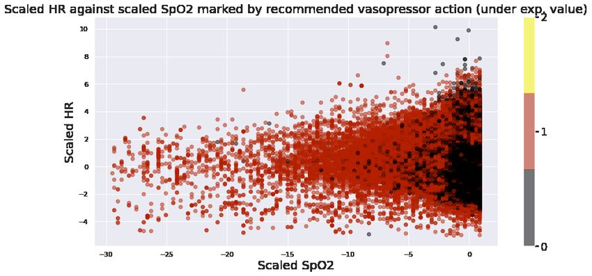
A PREPRINT

given state action pair. This random variable is certainly dependent on the training data, and the randomness stems from
the inherent randomness of stochastic gradient based optimization and random weights initialization. l is a divergence
metric appropriate for comparing probability distributions. We use the Kullback–Leibler divergence [48] for l.

4.4.1    Estimating the uncertainty measure
We find a Monte-Carlo estimate of this quantity, by bootstrapping 25 different datasets each substantially smaller than
the full training dataset, and training identical distributional RL algorithms in each. This can be done efficiently due to
the sample efficiency of distributional methods. And we can approximate E[θ] either by the ensemble value distribution,
or by the value distribution of the model trained on the full training dataset.

4.5     Uncertainty aware treatment

In previous work using distributional RL, the policy is selected with respect to the expected value. (i.e. The action
which has the highest expected value among all value distributions, is selected).
In this section we describe a general framework for choosing actions, which factors in model uncertainty.
Notice that, as our reinforcement learning algorithm learns (an approximation of) the optimal value distributions, making
decisions by considering additional information does not violate any assumption underlying the learning process.
When suggesting safe treatment strategies, we want the proposed action to have high expected value, however we also
would like our agent to flexible enough to propose an action with less model uncertainty, if two actions have very close
expected values, to each other. Another important factor to consider is how likely is an action to be taken by a human
clinician, although due to the nature of our 9 dimensional discrete action set this issue is significantly mitigated, as
opposed to a higher dimensional or continuous action space, we do want our propose action to be an action which is
considered likely by a human clinician.
To satisfy all three goals, we propose a general framework for choosing actions, based on a action preference score,
P(s, a) parameterized by three parameters. This general framework is flexible, yet simple, and the end user can choose
the parameters to reflect their own expert knowledge, and confidence of the model. Although this framework does
introduce additional parameters, and thus additional complexity, we propose suitable values for each parameter which
could be used as a fully automated, uncertainty aware decision support system.
First let’s define G(s, a), to be a human behavior likelihood score function. For our work we use the probabilities
outputted by the imitation learning network described in section 4.2.3.
Given a state s, we introduce P(s, a) associated with each action a, given by;

                                                          0                            0
                       P(s, a) = eβ1 (Q(s,a)−maxa0 Q(s,a )) + eβ2 (G(s,a)−maxa0 G(s,a )) − λu(s, a)                     (10)

where β1 > 0, β2 , λ ≥ 0, ,u(s, a) is the uncertainty associated with the state, action pair s, a and G(s, a) is the behavior
likelihood score.
λ penalizes, uncertainty, and a high β2 forces the action to be close to a clinician action. We could recover the expected
value criteria by setting β2 , λ = 0 and we could use the system as a pure behavior cloner, by setting β1 , λ = 0. The
first two terms of 10 belong to the interval (0, 1). Therefore β1 , β2 control how much away from the highest expected
value/behavior likelihood score can the agent choose an action from.
In choosing β1 , β2 , we also need to be cognizant of the scale of the scores used for behavior likelihood and the scale of
rewards. For a neural network which outputs log probabilities or probabilities we could use either, for our work we
chose the latter.
For our system, we propose β1 = 2, β2 = 1, λ = 0.05. We do reiterate that β2 = 1, depends on the fact that we use
probabilities (outputs of a softmax) as behavior scores, and thus much smaller in scale that the expected value. As
β2 → 0, the restriction of staying close to a clinician action gets more and more relaxed.

5     Results
We focus on RL results. We also briefly mention the reconstruction results of the physiology-driven autoencoder. The
results for one particular validation patient trajectory are presented in Figure 2. As the figure indicates, model has been
successful in reconstructing the observable outputs and their trends when the corruption probability was up to 25%. The
results do falter when the corruption level is too high, as illustrated by the output of our network when the trajectory

                                                              9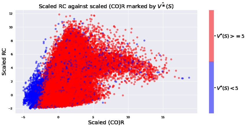
A PREPRINT

was corrupted with a 50% probability and fed to the network. This was typical among all patient trajectories, both for
training and validation datasets.

Figure 2: Reconstruction of a validation patient trajectory, using different levels of corruption using the physiology-driven autoencoder,
We have used a lower width for higher corruption rates for better visibility.

In analyzing our main work, we present results in three ways.
First as with any Machine Learning task it is essential to inquire about generalizability. We do this by investigating
value distributions of validation cohort patients. We further provide heuristic explanations of our models’ results by
showing the dependence on important input features, including identifiable cardiovascular states.
Then we consider individual, representative patients, (a) a survivor whose health deteriorated initially, and (b) a
non-survivor from our cohort, and analyze the expected value trajectories, uncertainty and treatment strategies for these
two patients.
Later we summarize global results, which include averaged treatment strategies and uncertainty patterns we could
observe empirically. However we note that at its core our approach strives to extract and then use patient specific
recurrent representations to learn personalized treatments. Therefore global analysis is unlikely to provide much insight
into the intricacies that underline the decision making process. Further when analyzing the proposed treatment, it
should also be noted that each action is proposed considering only the current, actual state. Therefore for a fixed patient
trajectory at a fixed time, the agent does not know what it has proposed previously, nor how it’s action would have
impacted the patient state.

5.1   Value distributions and expected values

We first investigate if the value distributions learned are generalizable, and if they are in agreement with clinical
knowledge. We further expect our networks to identify the mortality risk in advance, for patients who ended up dying at
the ICU.
For this purpose, we consider value distributions outputted for each time-step, for all our validation patients. Then we
group these distributions, by considering patients who died and patients who survived separately. We further group
these distributions by time to eventual death or discharge and consider the average distributions. Figure 3 shows these

                                                                   10
A PREPRINT
plots for 48, 24, 12 and 1 hour from death or discharge.4 We reiterate that our network only sees the patient state at a
given time, when it outputs the value distributions associated with the state. It is not provided with any information of
the future, the aggregation with respect to the time to death is done purely for analysis.
From Figure 3, we could observe a clear bi-modality for patients who died, even 48 hours in advance, and as the patient
state gets closer to eventual death, left peaks increase in area while the right peaks decrease, which results in the shift of
the expected values (centers of mass) of each distribution to the left. This agrees with the patient’s health deteriorating,
and at a certain point death becomes more likely an eventuality. We could also notice that the distribution associated
with no treatment has a larger left peak than others, highlighting that for these patient states lack of treatment for even
one hour could result in faster death.
In contrast, for survivors, peaks of the distributions maintain the same areas and their expected values remain closer to
the right limit. This again agrees with our expectation that when a patient is less than 2 days from eventual discharge, on
average their health state should be significantly healthier than non-survivors. And value distributions between different
actions are barely noticeable, which is reasonable considering a change in treatment for one hour may not significantly
alter the patient state, when a patient is at a less risky state.
We, next investigate the dependence of features and inferred states on the value distributions, and thus the optimal value
function V ∗ (s), computed as V ∗ (s) = maxa Q∗ (s, a).
Top figure of Figure 4, shows three scatter plots, between systolic blood pressure vs SOFA score, SpO2 vs Heart Rate
and RC vs (CO)R. In each scatter plot we mark points corresponding to V̂ ∗ (S) < 5 in blue and V̂ ∗ (S) ≥ 5 in red (5 as
a threshold was chosen arbitrarily, and we could observe similar results for any reasonable threshold). We can see a
perceptible separation of red and blue in each plot, and in each case this separation is consistent with medical knowledge.
For example low systolic blood pressure (hypotension) is associated with sepsis shock and higher mortality risk and
high SOFA scores indicate organ failure. Similarly as explained before, systemic vascular resistance, and cardiac output
both can be dramatically reduced close to death in septic patients. Therefore we could notice that our agent has learned
to discriminate between low risk (in the ICU context) and high risk septic patients states in an explainable manner. This
separation is more impressive when we consider that 89% of our patient states have the property V ∗ ≥ 5.
Further, the bottom figure of Figure 4, shows the same scatter plots, but now the marker color indicates the suggested
vasopressor treatment under expected value. (i.e. the treatment corresponding to the distribution which has the highest
expected value). These observations again agree with general goal of vasopressor treatment. Low systolic blood
pressure, low resistance, and cardiac output are all used as psychologic indications for vasopressor administration.
Next, we consider representative patients from our cohort, and analyze the expected values of all 9 distributions, and
model uncertainty for the patient trajectories. Top left figure of Figure 5, shows the evolution of expected values of all
nine actions each for a patient (ICU ID: 263969) who had died, with time. This was typical among all patients who
have died, initially there’s less variability among the expected values, especially the non-vasopressor actions are very
close in expected value, but as the patient’s health deteriorates the variation becomes more drastic, and there is a clear
preferences towards vasopressor based actions. We anecdotally observe that the difference between vasopressor based
treatment and non vasopressor based treatment becomes more significant whenever systolic blood pressure becomes
low and when the identifiable cardiovascular combination (CO)R becomes low. The marker size of each plot shows,
how much our agent is uncertain of its own results. (distribution associated with each state and action). We could also
observe that the model is less certain of its results when the patient’s health starts deteriorating. This can be attributed
to the fact that these states are uncommon in the dataset, and for septic patients the underlying cause behind health
deterioration could be very different. However when the patient is within 2 hours away from death, the uncertainty does
go down.
For comparison, the top right figure, of Figure 5 shows the evolution of expected values of a survivor (ICU ID: 279413
). Here we can notice that the expected values take a downward slide at around 25 hours from admission, with the
values associated with no treatment considerably lower. This coincides with SOFA score increasing, systolic blood
pressure,(CO)R rapidly decreasing, clearly indicating that the patient’s health has been deteriorating. However as SOFA
score improves (goes down), and the pressure and (CO)R goes up, as expected, expected values do go up, and now the
difference between expected values of each value distribution is considerably less. The uncertainty levels are also much
lower.
The fact that expected values of different actions being close to each other at healthy patient states, can be explained by
the RL framework. By equation 4, we can observe that Q∗ (s, a) is determined by the intermediate reward r(s, a, s0 )
and the next state s0 it transits to (because by definition we choose the optimal action at the next state s0 ). Further
our intermediate rewards are much smaller compared to terminal rewards. Therefore for a healthy patient state if the
4
For computational efficiency we only have considered a random subset of survivors, equal in size to the number of non survivors
11A PREPRINT
Figure 3: Value distributions for validation patients averaged according to different times from death or discharge, Top Non Survivors,
Bottom : Survivors
5
12A PREPRINT
Figure 4: Scatter plots of scaled features : Top : Marker colors indicates if V̂ ∗ (S) < 5 (Blue) or V̂ ∗ (S) ≥ 5 (Red) Bottom :
Marker colors indicate the vasopressor treatment under expected value
choice of action does not significantly change the next state in an hour, the Q functions would be close to each other.
Another way to interpret this is that a potentially wrong action can be reversed by taking the correct action in the next
hour if the patient is non critical, however if the patient is at a more critical state a wrong action can have more drastic
consequences.
In the appendices, we also present the evolution of expected values of 6 validation patients.
The results presented in this section indicate that our network, has learned generalizable value distributions, which in
most cases identify the risk of death considerably before eventual death. And since our treatment strategies are based on
the learned value distributions, we have confidence that the learned policies will also be generalizable.
13A PREPRINT
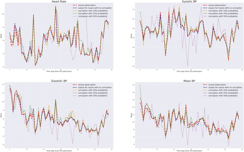
Figure 5: Top : Expected value evolution for two patients Left :A patient who died in the ICU. The marker size indicates the
uncertainty associated with a particular action. Also shown are the standardized values of SOFA score, Systolic blood pressure, and
the unidentifiable cardiovascular state (CO)R. x axis indicates the hours from ICU admission. Right : A survivor, Same comments as
above. Bottom : Recommended actions under various combinations of β1 ,β2 and λ, for the same two patients Left : Non Survivor,
Right : Survivor x axis :the time in hours from ICU admission,y axis: the discretized action a : Recommended actions under
expected value and behavior cloning, b: λ=0.1 and β1 , β2 is varied, c :β1 = 2, β2 = 1 and λ is varied, d : Clinician Action
a
b
c
d
14A PREPRINT
5.2 Model uncertainty
In this section, we briefly mention results of uncertainty quantification.
In Figure 8 (Appendix C) we provide radar plots of uncertainty measures associated with each action, for randomly
generated patients, at various times throughout their ICU stay. The common pattern is that for most patients who have
died, the model is less confident about its value distributions as they become closer to death. Uncertainty among each
action varies from patient to patient. However for survivors this behavior is the exact opposite, as the agent is more
confident of its results and becomes even more confident as the patient gets closer to discharge from the ICU.
Appendix C also presents summary statistics of uncertainty results for survivors and non-survivors.
As we mentioned previously and also detailed out in the appendix, this behavior is not surprising since death states
are relatively uncommon, and also there are a wide variety of ways a septic patient may face increased mortality risk.
However for survivors, we do expect all of them to approach a healthy state as they approach eventual discharge.
5.3 Uncertainty aware treatment
In this sub-section we present treatment strategies for patients made by the model. As mentioned before one should be
cognizant of the Markovian assumption of the agent (as with all RL agents) when interpreting the results.
First we will consider the two patients we considered under value distributions (presented at the top of Figure 5), and
analyze the suggested treatment under various parameter combinations. These results are presented at the bottom of the
Figure 5. Left figures correspond to the non-survivor and the right figures correspond to the survivor.
First, panels (a) (of both left and right figures) show the treatments under expected value, and behavior cloning
respectively (corresponding to β1 6== 0, β2 = 0 and λ = 0, and β2 6== 0, β1 = 0 and λ = 0).
To facilitate better comparison we fixed β1 = 2, and consider different levels of β2 and λ. Panels (b) keeps β1 = 2, λ =
0.1, fixed and varies β2 , whilst panels (c) vary λ keeping the first two fixed.
By considering the bottom left figures we can notice that just as we discussed in the previous sub-section, as the
patient’s health deteriorates, (evinced by the sharp fall in systolic blood pressure, (CO)R, and increase in SOFA score),
vasopressors are recommended by all of the combinations.
The figure on the right, whilst much harder to interpret we could again notice, that around 20-30 hours, and 40-50 hours
vasopressors are proposed, this coincide with the steep downward slide of SBP and (CO)R.
For comparison with previous work in RL for sepsis treatment [14], we also provide heat-maps of clinician’s and agent’s
proposed treatments separately for, overall, low SOFA ( 0, pushes the treatments closer, to the clinician’s treatment.
As mentioned above however, these kind of global averaged treatment analysis may not reflect the intricacies underlying
the decision recommending system, as our methods all are individualized.
5.4 A comment on Off Policy Evaluation
Off policy evaluation, is the quantitative or statistical evaluation of the value of a learned policy, using another dataset,
usually a validation cohort.
Although this is attractive in theory, most common unbiased off policy value estimates, depend on the behavior policy,
which generated the data being known. However this is not the case when the data was generated by human clinicians’
actions. It could be argued that the behavior cloner could be used as an approximate behavior policy, however it is
trained to predict the likely clinician action, and it’s unlikely to be a good approximator to be used as a stochastic
behavior policy.
Further previous research has claimed at all off policy evaluation methods are unreliable in the sepsis management
context [49]. These problems are exacerbated when the policy which is to be evaluated is deterministic.
Due to the above reasons we do not consider statistical off policy evaluation in this work, however we note that
developing off policy evaluation techniques suited for the critical care domain is a very important area of research to
explore in the future.
15A PREPRINT
Figure 6: L : Heat-plots for recommended actions, under β1 = 2,β2 = 1,lλ = 0.05 and Expected Values, Shown are cinician’s vs
Agent for overall (orange), low sofa (green), medium sofa (blue), high score (purple) and non survivors (red).
16A PREPRINT
6 Discussion
We present an inter-disciplinary approach which we believe takes a significant step towards improving the current state
of data-driven interventions in the context of clinical sepsis (both in terms of end goals and interpretability), as well as
automated medical decision support. We believe, the maximum benefit of Artificial Intelligence applied to medicine,
can be realized when used in conjunction with traditional sciences and engineering, as well maximizing human expert
knowledge.
Our contribution improves the status quo several ways. Compared to prior work, our approach deals with partial
observability of data, yet known physiology, by leveraging a low-order two-compartment Windkessel-type cardiovascular
model to extend the state space, and deriving insight from recent advances in self-supervised representation learning.
As mentioned previously, this has several benefits. In the context of sepsis treatment, cardiovascular states are crucial
in obtaining an accurate physiologic state for patients. Indeed, the clinical decision to administer intravenous fluids
or vasopressor is driven by an implicit differential diagnosis, on behalf of the clinician, as to whether insufficient
organ perfusion and shock are secondary to insufficient circulating volume (thus administer fluids), vasoplegia (thus
administer vasopressors), or some combination of both fundamental pathophysiology. There is typically insufficient
data to determine whether heart function is adequate (contractile dysfunction), but this could also be included in the ab
initio physiologic model if prior knowledge was present. Further the incorporation of physiologic models improves
model explainability, while deep neural networks and stochastic gradient-based optimizers make it possible to learn
robust and generalizable representations from large data. We expect the unification of first principle based models, and
data driven approaches such as deep networks will provide a powerful interface between traditional computational
sciences and modern machine learning research, mutually benefiting both disciplines.
We also introduce an approach to model uncertainty which, as we have explained in detail, is essential in any practical
application of RL-based inference using clinical data. To the best of our knowledge, this is the first time uncertainty
quantification is used to quantify epistemic uncertainty in RL-based optimization of sepsis treatment, and of critical
care applications more generally. 6 .
We propose a simple framework for automated decision making support which considers model uncertainty, and
behavior likelihood. This principle again aligns with the deeper idea of combining different expertise and knowledge
for better decision making, a philosophy consistent with the rest of this work.
There are additional interesting observations. We chose a decision time step of one hour. Compared to similar work,
this is much more compatible with the time scale of medical decision making in sepsis, where fluid and vasopressor
treatments are titrated continuously, at least theoretically. Accordingly, on such a time scale, there does not appear to be
large differences in the relative merit of different dosing strategies. This makes intuitive sense: there is presumably a
lesser need for major treatment modifications if decisions are made more frequently. Yet, a frequent finding across
patients, especially the sickest ones, was that doing nothing was a consistently worse strategy. This also meets clinical
intuition.
Reducing the time scale of decisions is not only appealing clinically in situation of rapidly evolving physiological states
such as is the case in early sepsis, but it also provides a more compelling basis for a less granular action space. Indeed,
if decisions are make hourly, it does meet clinical intuition to have fever discrete actions: Few physicians will argue that
there is likely to be little difference in administering 100cc or 200cc of fluids in the next hour. In the extreme, if time
were continuous, the likely decision space, at any given time, is whether a fluid bolus should be administered or not. A
similar reasoning applies to vasopressors (increase, reduce, status quo).
We have shown that our methods, have learned clinically interpretible value distributions, which can be computed
sequentially using data routinely calculated at the ICU. These value distributions quantify the mortality risk associated
with a septic patient, and thus can be used as risk score.
6.1 Future Work
There are other avenues we would like to explore.
Model-based RL with physiological models: Model-based RL aims to explicitly model the underlying environment
and then use this information in various ways in figuring out control strategies. 7 This paradigm provides a natural
place to incorporate mechanistic models, which could potentially help both control and interpretability. Clearly, the
availability of more granular data, or of additional domains of data, could allow better estimation of the underlying
physiological model and thus reduce uncertainty.
6
Previous approaches e.g.: [31] have considered inherent environment uncertainty
7
It could in theory be argued that our work itself is a model based and model free hybrid method.
17A PREPRINT
Reward Structure: Our reward structure was based on previous work and has clinical appeal. However, rewards are
an essential component of any RL algorithm and is the only place where the agent can judge the merit of its proposed
actions. This is potentially another place to include physiological knowledge. Ideally, we would want our reward
structure to capture an accurate mortality risk, and an organ damage score, with each state. Risk-based rewards, rooted
in anticipated evolution over a meaningful clinical horizon, should be considered in future schemes.
References
[1] Chanu Rhee, Raymund Dantes, Lauren Epstein, David J Murphy, Christopher W Seymour, Theodore J Iwashyna,
Sameer S Kadri, Derek C Angus, Robert L Danner, Anthony E Fiore, et al. Incidence and trends of sepsis in us
hospitals using clinical vs claims data, 2009-2014. Jama, 318(13):1241–1249, 2017.
[2] PE Marik. The demise of early goal-directed therapy for severe sepsis and septic shock. Acta Anaesthesiologica
Scandinavica, 59(5):561–567, 2015.
[3] Alexandra Lazăr, Anca Meda Georgescu, Alexander Vitin, and Leonard Azamfirei. Precision medicine and its
role in the treatment of sepsis: a personalised view. The Journal of Critical Care Medicine, 5(3):90–96, 2019.
[4] Ivor S Douglas, Philip M Alapat, Keith A Corl, Matthew C Exline, Lui G Forni, Andre L Holder, David A
Kaufman, Akram Khan, Mitchell M Levy, Gregory S Martin, et al. Fluid response evaluation in sepsis hypotension
and shock: A randomized clinical trial. Chest, 2020.
[5] P Marik and Rinaldo Bellomo. A rational approach to fluid therapy in sepsis. BJA: British Journal of Anaesthesia,
116(3):339–349, 2016.
[6] Vincent Liu, Gabriel J Escobar, John D Greene, Jay Soule, Alan Whippy, Derek C Angus, and Theodore J
Iwashyna. Hospital deaths in patients with sepsis from 2 independent cohorts. Jama, 312(1):90–92, 2014.
[7] Richard S. Sutton and Andrew G. Barto. Reinforcement Learning: An Introduction. MIT Press, 1998.
[8] Volodymyr Mnih, Koray Kavukcuoglu, David Silver, Andrei A Rusu, Joel Veness, Marc G Bellemare, Alex
Graves, Martin Riedmiller, Andreas K Fidjeland, Georg Ostrovski, et al. Human-level control through deep
reinforcement learning. nature, 518(7540):529–533, 2015.
[9] David Silver, Aja Huang, Chris J Maddison, Arthur Guez, Laurent Sifre, George Van Den Driessche, Julian
Schrittwieser, Ioannis Antonoglou, Veda Panneershelvam, Marc Lanctot, et al. Mastering the game of go with
deep neural networks and tree search. nature, 529(7587):484–489, 2016.
[10] Florian Fuchs, Yunlong Song, Elia Kaufmann, Davide Scaramuzza, and Peter Duerr. Super-human performance
in gran turismo sport using deep reinforcement learning. arXiv preprint arXiv:2008.07971, 2020.
[11] Siqi Liu, Kay Choong See, Kee Yuan Ngiam, Leo Anthony Celi, Xingzhi Sun, and Mengling Feng. Reinforcement
learning for clinical decision support in critical care: comprehensive review. Journal of medical Internet research,
22(7):e18477, 2020.
[12] Chao Yu, Jiming Liu, and Shamim Nemati. Reinforcement learning in healthcare: A survey. arXiv preprint
arXiv:1908.08796, 2019.
[13] Matthieu Komorowski, Leo A Celi, Omar Badawi, Anthony C Gordon, and A Aldo Faisal. The artificial
intelligence clinician learns optimal treatment strategies for sepsis in intensive care. Nature medicine, 24(11):1716–
1720, 2018.
[14] Aniruddh Raghu, Matthieu Komorowski, Imran Ahmed, Leo Celi, Peter Szolovits, and Marzyeh Ghassemi. Deep
reinforcement learning for sepsis treatment. arXiv preprint arXiv:1711.09602, 2017.
[15] Xuefeng Peng, Yi Ding, David Wihl, Omer Gottesman, Matthieu Komorowski, Li-wei H Lehman, Andrew Ross,
Aldo Faisal, and Finale Doshi-Velez. Improving sepsis treatment strategies by combining deep and kernel-based
reinforcement learning. In AMIA Annual Symposium Proceedings, volume 2018, page 887. American Medical
Informatics Association, 2018.
[16] Megan A Rech, Megan Prasse, and Gourang Patel. Use of vasopressors in septic shock. JCOM-Journal of Clinical
Outcomes Management, 18(6):273, 2011.
[17] Jason Waechter, Anand Kumar, Stephen E Lapinsky, John Marshall, Peter Dodek, Yaseen Arabi, Joseph E Parrillo,
R Phillip Dellinger, Allan Garland, Cooperative Antimicrobial Therapy of Septic Shock Database Research Group,
et al. Interaction between fluids and vasoactive agents on mortality in septic shock: a multicenter, observational
study. Critical care medicine, 42(10):2158–2168, 2014.
[18] JD Young. The heart and circulation in severe sepsis. British journal of anaesthesia, 93(1):114–120, 2004.
18You can also read