Stimulating Implementation of Sustainable Development Goals and Conservation Action: Predicting Future Land Use/Cover Change in Virunga National ...
←
→
Page content transcription
If your browser does not render page correctly, please read the page content below
sustainability

Article
Stimulating Implementation of Sustainable
Development Goals and Conservation Action:
Predicting Future Land Use/Cover Change in Virunga
National Park, Congo
Mads Christensen and Jamal Jokar Arsanjani *
 Geoinformatics Research Group, Department of Planning and Development, Aalborg University Copenhagen,
 A.C. Meyers Vænge 15, DK-2450 Copenhagen, Denmark; madc@dhigroup.com
 * Correspondence: jja@plan.aau.dk

 Received: 7 December 2019; Accepted: 12 February 2020; Published: 19 February 2020

 Abstract: The United Nations 2030 Agenda for Sustainable Development and the Sustainable
 Development Goals (SDG’s) presents a roadmap and a concerted platform of action towards achieving
 sustainable and inclusive development, leaving no one behind, while preventing environmental
 degradation and loss of natural resources. However, population growth, increased urbanisation,
 deforestation, and rapid economic development has decidedly modified the surface of the earth,
 resulting in dramatic land cover changes, which continue to cause significant degradation of
 environmental attributes. In order to reshape policies and management frameworks conforming
 to the objectives of the SDG’s, it is paramount to understand the driving mechanisms of land use
 changes and determine future patterns of change. This study aims to assess and quantify future land
 cover changes in Virunga National Park in the Democratic Republic of the Congo by simulating a
 future landscape for the SDG target year of 2030 in order to provide evidence to support data-driven
 decision-making processes conforming to the requirements of the SDG’s. The study follows six
 sequential steps: (a) creation of three land cover maps from 2010, 2015 and 2019 derived from satellite
 images; (b) land change analysis by cross-tabulation of land cover maps; (c) submodel creation
 and identification of explanatory variables and dataset creation for each variable; (d) calculation of
 transition potentials of major transitions within the case study area using machine learning algorithms;
 (e) change quantification and prediction using Markov chain analysis; and (f) prediction of a 2030 land
 cover. The model was successfully able to simulate future land cover and land use changes and the
 dynamics conclude that agricultural expansion and urban development is expected to significantly
 reduce Virunga’s forest and open land areas in the next 11 years. Accessibility in terms of landscape
 topography and proximity to existing human activities are concluded to be primary drivers of these
 changes. Drawing on these conclusions, the discussion provides recommendations and reflections on
 how the predicted future land cover changes can be used to support and underpin policy frameworks
 towards achieving the SDG’s and the 2030 Agenda for Sustainable Development.

 Keywords: land cover modelling; remote sensing; machine learning; sustainable development goals;
 Virunga National Park

1. Introduction
     Established in 1925 as the first National Park (NP) in Africa, the Virunga NP is located in the
Albertine Rift Valley in the eastern part of the Democratic Republic of the Congo [1]. Along with the
Mgahinga Gorilla NP in Uganda and the Parc Nationale Des Volcans in Rwanda, Virunga is part of a
triangle of NP’s in central Africa, principally designated in order to enhance conservation efforts to

Sustainability 2020, 12, 1570; doi:10.3390/su12041570                    www.mdpi.com/journal/sustainability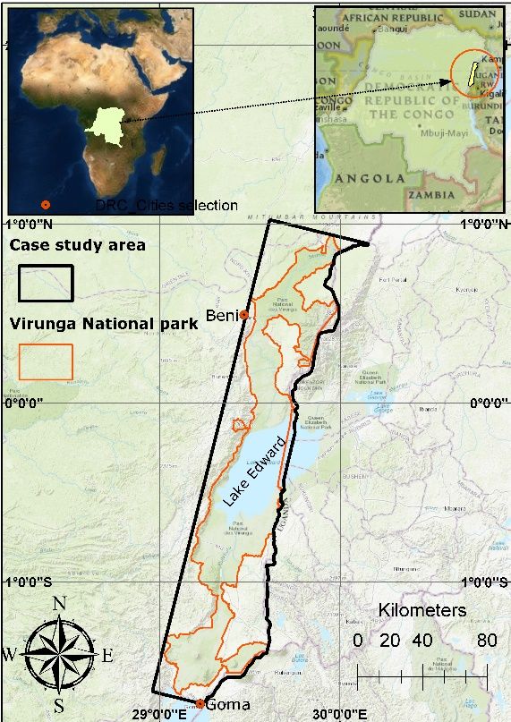
Sustainability 2020, 12, 1570                                                                        2 of 28

protect the critically endangered mountain gorilla (Gorilla Beringei Beringei) [2]. The park covers an area
of 790,000 ha [3], and hosts the majority of the fragments of the last remaining habitat suitable for the
mountain gorilla. Furthermore, the multitude of variety in nature and climate variables, including large
lakes, open land savannah, vast forest areas, snow-covered mountain tops and erupting volcanoes,
provides critical habitats for a great variety of the other large species of mammals we associate with
Africa [1]. For this reason, the park was inscribed as a United Nations (UN) Educational, Scientific and
Cultural Organization (UNESCO) World Heritage site in 1979. However, the NP is located in one of the
most densely populated regions in sub-Saharan Africa, which has been the scene of prolonged political
turmoil and social conflict [4], causing severe pressure on the ecological integrity of the landscape and
its biodiversity. Moreover, the rich volcanic soil and high rainfall within the Virunga NP catchment
makes it highly suitable for agriculture, and thus an attractive opportunity to underpin subsistence
and commercial farming operations [2].
      The rapidly increasing population has significantly increased the demand for natural resources
(land, water energy, food, etc.), causing rapid land clearing for agriculture and grazing, removal of
plants for different purposes, including artisanal mining operations, and house building [4]. Despite the
efforts of authorities to protect the integrity of the NP, multiple pressures continue to threaten its
habitats and biodiversity, including: civil unrest; illegal activities; land conversion and encroachment;
livestock farming / grazing of domesticated animals; widespread depletion of forests in the lowlands
and; a massive influx of 1 million refugees occupying adjacent areas of the park [5]. Militia leaders and
prospectors are threatening the borders of the park in search for the vast deposits of diamonds, gold,
uranium and other coveted minerals, while the vast influx of destitute refugees resorts to poaching and
charcoal production, resulting in further fragmentation and degradation of the forest landscape [1].
In fact, the majority of the total population of nearly 6 million people in the surrounding province of
North Kivu rely entirely on charcoal for their cooking needs, and an estimated three-quarter of this
charcoal is sourced from the Virunga catchment, most of it illicitly from within the NP [6].
      Thus, the region is highly important, both ecologically and economically, and the conflicting
demands for socioeconomic development while maintaining the ecological integrity of the NP has
underpinned the need to ensure continued conservation efforts and sustainable natural resource
management. This is critical in order to safeguard the biodiversity and habitats of the NP,
while preserving the foundation of the livelihoods of millions of people. This agenda is fortified
through the UN 2030 Agenda for Sustainable Development and the 17 Sustainable Development Goals
(SDG)’s that were adopted at the UN general assembly in 2015. The SDG’s call on concerted action to
pursue economic development while ensuring social inclusion and environmental sustainability on the
basis of good governance. The SDG framework provides a comprehensive agenda through which to
mainstream policies and derive targeted actions for addressing core sustainability challenges. However,
the ability to target policies and actions to address conservation issues, while pursuing economic
development and prosperity, leaving no one behind, is hampered by lacking scientific evidence and
data to direct and support informed decision making.
      In order to derive targeted policies and actions to support effective land use planning, management
and ecological restoration conforming to the requirements of the SDG’s, it is imperative to understand
the underlying processes of change [7]. Up-to-date information on current land cover and land use
provides critical information that can be used to underpin decision-making processes, while modelled
predictions about plausible future land use/land cover (LULC) scenarios provide indications of potential
trajectories and thus a platform for identifying interventions. Changes in land use and land cover
can be described and projected through the use of land change models, which can be used to explain
and assess the dynamics of land cover- and broader system change [8]. Spatial land change models
thus provide platforms for exploring potential future scenarios, which can be used to guide land use
decision making and planning [8].
      The purpose of the study is to assess and quantify past and plausible future land use and land
cover changes and dynamics within the Virunga case study area. The primary analysis will be guided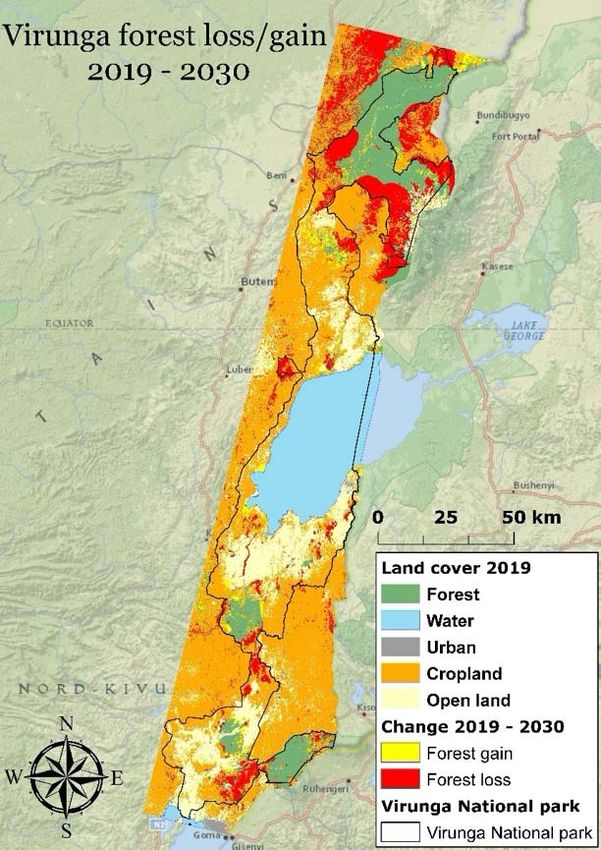
Sustainability 2020, 12, 1570                                                                                                                3 of 28

by a change analysis of classified satellite imagery to quantify past changes, and the development of a
land change model, applying a coupled machine learning—the Markov chain approach—to derive
a future land cover prediction for the year 2030. The aim is to assess the plausible future evolution
of the landscape within the Virunga case study area and address an existing data gap in order to
provide evidence to support data-based decision-making processes conforming to the requirements of
the SDG’s.

Problem Statement and Research Questions
     While several studies have already successfully applied predictive land change modelling to
support land use management and decision-making processes [9–12], a thorough literature review
indicates that such an approach has been applied in just a few case studies and hence it is necessary to
explore further cases in order to assure its applicability across different landscapes. Therefore, a remote
area is targeted in Africa covering the Virunga NP and its immediate vicinity. This study aims to apply
remotely sensed data and geospatial and modelling tools to detect, quantify, analyse, and predict future
land change in the Virunga NP and its immediate vicinity. Hence, the following research questions are
targeted:

•     Have there been major land cover changes within the study area in the last 10 years? And if so,
      what kind of land cover changes?
•     What has the spatial extent of the land cover change been and which areas have experienced the
      highest rate of changes?
•     What are the major driving forces behind these changes?
•     What will the extent of land change be by 2030?
•     How can the future land cover prediction for the Virunga study area be used to support and
      underpin policy frameworks towards achieving the SDG’s?

2. Study Area
     The Virunga NP is located in Central Africa, in the Eastern part of the Democratic Republic of
the Congo, on the border with Uganda and Rwanda. It is located in the equatorial zone, within the
Albertine Rift, of the Great African Rift Valley [3]. In this study, The Virunga NP and its immediate
vicinity was used as case study area in order to assess the dynamics within the NP and the landscape
dynamics of the entire Virunga catchment. The study area is created from a minimum-bounding
rectangle encompassing the entire NP, clipped at the Rwandan border. It was considered critical to
include the border areas around the NP in order to explore socioeconomic changes, primarily in the
form of urban development and cropland expansion, outside of the NP, and assess how these land
cover dynamics could potentially impede conservation efforts and sustainable land management
planning. The study area, as shown in Figure 1, covers a total of 14,810 km2 of which 7779 km2 is
within the Virunga NP.
                                Sustainability 2020, 11, x FOR PEER REVIEW                                                         4 of 31

                                             Figure 1. Study area around the Virunga NP in the Democratic Republic of the Congo.
               Figure 1. Study area around the Virunga NP in the Democratic Republic of the Congo.
                                3. Methodology
                                    The methodological framework utilized in this study to predict the future landscape around the
                                Virunga NP was developed using a variety of different tools and the theoretical framework outlined
                                below. The workflow is illustrated in Figure 2.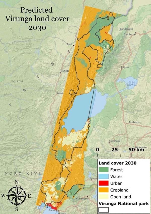
Sustainability 2020, 12, 1570                                                                          4 of 28
               Figure 1. Study area around the Virunga NP in the Democratic Republic of the Congo.

3. Methodology
    The methodological framework utilized in this study to predict the future landscape around the
Virunga NP
Virunga NP was
            was developed
                developed using a variety of different
                                                different tools
                                                          tools and
                                                                and the theoretical framework outlined
below. The workflow is illustrated
below.                 illustrated in
                                   in Figure
                                      Figure 2.
                                             2.

           Figure 2.
           Figure    Land Change
                  2. Land Change Modelling
                                 Modelling workflow
                                           workflow to
                                                    to predict
                                                       predict land
                                                               land cover
                                                                    cover change
                                                                          change in
                                                                                 in Virunga
                                                                                    Virunga in
                                                                                            in 2030.
                                                                                               2030.

     In this section, the methodology applied in this study to derive land cover predictions for the year
2030, conforming to this sequential stepwise approach is described. All datasets were either created
in, or re-projected to, a Reseau Geodesique de la République Democratique du Congo (RDC) 2005
Transverse Mercator (TM) Zone 18 (EPSG:4051) projected coordinate system, recommended for use in
the Democratic Republic of the Congo. ArcGIS was used as a primary tool for data preprocessing and
visualisation of results.

3.1. Land Cover Classification
     Google Earth Engine provides a cloud-based platform for accessing and processing large amounts
of both current and historical satellite imagery, including those acquired by the Landsat-7 and Landsat-8
satellites. The advantages of seamless integration of archived, and pre-processed satellite imagery,
along with a powerful cloud-processing platform made Google Earth Engine an ideal platform for
conducting the land cover classification. The land classification in Google Earth Engine is composed of
several different steps;

•     Choosing an appropriate satellite imagery dataset, fitting the objective of the study,
•     Define land cover classes and collect training data to train the supervised classification algorithm,
•     Developing a JavaScript code to acquire, process and classify the satellite imagery based on the
      choice of classification algorithm.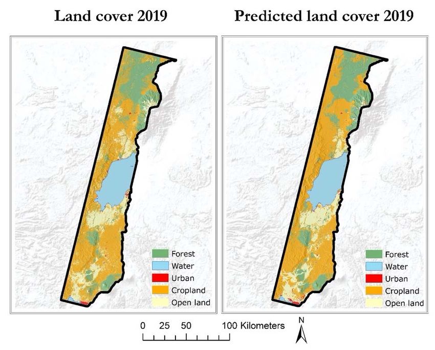
Sustainability 2020, 12, 1570                                                                                   5 of 28

3.1.1. Satellite Imagery
     In this study, three land cover maps were created, one for 2010, 2015 and 2019. As the National
Aeronautics and Space Administration (NASA)’s Landsat satellites provides an archived and freely
available dataset covering the entire study period with high resolution (30 m) multispectral imagery,
these were selected for this study. Google Earth Engine provides integrated access to analysis-ready
(already geometrically corrected and orthorectified), surface reflectance Landsat data from the Tier-1
collection. For the 2010 land cover map, tier-1 data from the Landsat 7 Enhanced Thematic Mappers
(ETM+) sensor were selected, while tier-1 data from the Landsat 8 Observation Land Images (OLI) were
chosen for the 2015 and 2019 land cover maps. For all three land cover maps, cloud-free composite
images were generated from a stack of multiple images collected from the preceding three years (i.e.,
the 2010 land cover map is based on images from 2008–2010). Only images with less than 30% cloud
cover were used in the compositing process, resulting in approximately 60–70 useable tiles for each
three-year period.

3.1.2. Collecting Training/Validation Data
      As a first step in preparing a training dataset for the land classification, the definition of a
nomenclature of land cover classes fitting the objective of the study needed to be defined. Accordingly,
the 5 following land cover classes were enough to ensure a sufficient representation of the spatiotemporal
variety of land cover changes and identify the primary drivers contributing to forest change dynamics.

1.     Forest: afforested and primary forest areas. (Note: While the authors acknowledge the significant
       difference between afforested areas and primary forest, further separation of the two classes would have
       caused significant classification errors, due to the spectral similarity of the two classes. Accordingly, the
       two classes were merged into a combined forest cover class to increase classification accuracy of forest cover.)
2.     Water: lakes and rivers.
3.     Urban areas: developed residential or industrial areas, roads and urban fringes.
4.     Cropland: planted or bare crop fields.
5.     Open land/grassland: areas with sparse vegetation, characterized by open grasslands, bare soil or
       volcanic ash.

      To train and validate the land-cover classifications, a reference training dataset was collected
within the study area. The minimum samples for machine learning based algorithms to perform
optimally should be at least 10 times the number of land cover classes. Thus, the training data samples
should be at least 50. These reference training datasets were collected by drawing polygons and
clicking points within the Google Earth Engine map interface. The points and polygons were randomly
collected throughout the case study area, collecting multiple instances of training data samples for
each land cover class. From the collection of training data polygons and points, a subsample of
500 points was used to train the model. An additional point dataset consisting of 50 individually
sampled points were collected and used for validation. The validation dataset (i.e., ground truth) was
sampled using high-resolution images available in the Google Earth archive from representative years
between 2010–2019.

3.1.3. Land Cover Classification within the Google Earth Engine IDE
     In order to create the three land cover maps, three individual scripts were prepared within
the Google Earth Engine Integrated Development Environment (IDE), one for each of the three
years. The JavaScript source code for the land cover classification is included in the Appendix A.
The first component of the script was to import the area of interest (AOI) as table data. Secondly,
five empty containers for geometry collections for the training datasets were imported as variables.
Subsequently, the cloud-free composite of satellite images was imported using the JavaScript code.
The function ‘maskClouds’ generates a cloud and a cloud shadow mask for the imported Landsat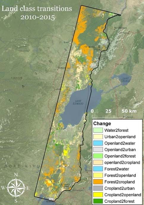
Sustainability 2020, 12, 1570                                                                                                       6 of 28

collection. Furthermore, within this function, the Normalized Difference Vegetation Index (NDVI)
was calculated and added to the band collection of the satellite image composite. The NDVI was
added to the band collection to enhance the contribution of vegetation in the spectral response for
the classification. In addition to NDVI, the first seven bands of the Landsat 8 composite were used in
the classification algorithm for the 2015 and 2019 land cover maps. Bands 1-5, band 7 and the added
NDVI band were used for the 2010 land cover map, based on the Landsat 7 composite. Thereafter,
500 sample points for each training layer were generated by looping over each training dataset and
creating random points within the geometries of the training data layers. Lastly, a confusion matrix
was created in order to assess the performance of the classification algorithm.

3.2. LULC Modelling and Prediction
    The Land Change Module (LCM) within TerrSet (Geospatial Monitoring and Modeling Software)
was used to conduct the sequential steps conforming to the requirements of LULC modelling using a
multi-layer perceptron (MLP)-Markov chain approach. In this section, each step of the LULC modelling
process is described.

3.2.1. Modelling Transition Potentials: Submodels
     The second step in the LULC change prediction process is to model the transition potentials,
which are in essence maps of suitability/likelihood of one land cover changing into another [13].
Following [14] the land cover transitions can be grouped together into empirically evaluated transition
submodels when the common underlying drivers are assumed to be the same. The submodels can
consist from a single land cover transition (e.g., from open land to cropland) or from multiple transitions,
grouped together based on the assumption that transitions are caused by the same underlying drivers
of change. The explanatory variables are used to model the historical change process based on the
empirical relationship between the measured change and the explanatory variable.
     Based on the major land class transitions identified in the previous step, the 12 predominant
transitions were grouped together based on transition type to form six individual submodels.
The composition of transition groups and a description of the types of changes under each submodel
can be seen in Table 1. Although persistence, i.e., areas that did not change, can be considered a
trajectory, it cannot be considered as a transition class, and thus areas of persistence are ignored in
LCM [10].

                                       Table 1. Transition submodels and descriptions.

       Transition Submodel                                    Description                                   Land Cover Transitions

                                                                                                        •     Urban to open land
     Abandonment/reclamation        Urban and agricultural areas converted to grassland and open land
                                                                                                        •     Cropland to open land

                                                                                                        •     Cropland to forest
            Afforestation                    Land cover classes converted to tree plantation
                                                                                                        •     Open land to forest

     Agricultural intensification     Agricultural areas substituting grasslands and open land areas    •     Open land to cropland

                                                                                                        •     Forest to cropland
            Deforestation                  Forested areas converted into other land class types
                                                                                                        •     Forest to open land

                                                                                                        •     Forest to water
         Natural dynamics                  Areas where natural changes cause land conversion            •     Water to forest
                                                                                                        •     Open land to water

                                                                                                        •     Cropland to urban
        Urban intensification                   Urban areas substitute other land classes
                                                                                                        •     Open land to urban

3.2.2. Explanatory Variables
    LULC change processes are dynamic and result from the interaction between a range of different,
primarily biophysical and socioeconomic criteria. In LULC change modelling, these criteria are also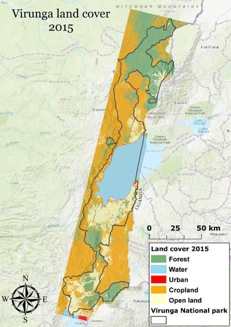
Sustainability 2020, 12, 1570                                                                         7 of 28

referred to as ‘explanatory’ variables, as these explain the components of the causal relationships
determining the land cover dynamics and they form a critical prerequisite for developing a realistic
land change model. The explanatory variables sum up the “knowledge” that the model will use
to simulate future land cover scenarios [15]. Each explanatory variable was tested for its potential
explanatory value using Cramer’s V scores. Cramer’s V is a coarse statistic measure of the strength of
association or dependency between two variables and it ranges from 0.0 to 1.0 in values. Generally,
variables with a total Cramer’s V score higher than 0.15 are considered useful and those with a score
over 0.4 are considered good [13].
      In choosing explanatory variables, the processes contributing to land cover change needs to be
visualised in the form of a spatial dataset representing the underlying changes, at a spatial resolution
consistent with the land cover maps (30 m). GIS data sets (further described in Table 2) were identified
to describe the transitions in the case study area and geoprocessing was performed to derive spatial
datasets to, either directly or as a proxy, explain the underlying changes for each transition. According
to [16] variables cannot be categorical and thus needs to be continuous and quantitative. The drivers
that were used in this study include; elevation (Digital Elevation Model (DEM)), aspect (Asp), slope,
Evidence Likelihood (EL), distance from artisanal mines (D_am), distance from disturbance (D_disturb),
distance from cities (D_cities), distance from forests (D_forest), distance from mining concessions
(D_mining), distance from roads (D_roads), distance from waterways (D_water).
      For each land cover class, evidence likelihood answers the question, “How likely is it that you would
have this if you were an area that would experience change?” [13], meaning that it established the
suitability of each pixel to transform into urban areas or cropland. To do this, evidence likelihood
transforms a categorical variable into a continuous surface, based on the relative frequency of pixels
belonging to the different categories within the areas of change [17]. In this study, evidence likelihood
is a quantitative measure of the frequency of change between urban areas and cropland (also called
disturbance) and all other land classes from 2010–2015. Thus, it represents the relative frequency of the
different land cover classes that occurred in the areas that transitioned to urban or cropland. This variable
aims to explain the geospatial processes that determine urban expansion and agricultural intensification.
      The distance drivers represent the proximity of pixels to forces that either constraints or incentivise
land cover changes. Mining activities is one of the primary driver of deforestation within the Virunga
area “Artisanal mining operations are unregulated and often occur in riparian zones, removing forest and
vegetation cover to process the mineral soil.” [18]. Accordingly, there is a documented relationship between
deforestation and mining operations, thus, distance from artisanal mines and distance from mining
concessions are included as proxy drivers of forest conversion, the rationale being that the closer
in proximity a forested area is to known mining operations, the more likely it is to be deforested.
Likewise, these drivers will likely positively correlate with an increase of open land, urban areas
and cropland nearer to the mining concessions. Distance to disturbance is a spatial driver made from
extracting Euclidian distances from areas that were urban or cropland in 2010. The hypothesis is that
future anthropogenic disturbance is believed to be closer to areas of existing disturbance, and thus
distances to existing disturbances are believed to be closely correlated with urbanisation processes and
agricultural expansion.
      Table 2 below describes the input datasets as well as the geoprocessing steps of each of the
explanatory variables.
Sustainability 2020, 12, 1570                                                                                                                                                                                                                  8 of 28

                                                                                 Table 2. Description of potential explanatory variables.
      Variable         DEM              Asp         Slope          EL                D_am                  D_disturb              D_cities             D_forests               D_mining                   D_roads                 D_water
                                                                              International Peace
                                                               Land cover                                                     World Resources
     Data origin    SRTM 90m Digital Elevation Database v4                    Information Service        Land cover 2010                            Land cover 2010                                World Resources Institute
                                                               2010 + 2015                                                       Institute
                                                                                     (IPIS)
                                                                 Raster            Shapefile                                      Shapefile                                    Shapefile                  Shapefile               Shapefile
    Data format                  Raster (GeoTiff)                                                        Raster (GeoTiff)                           Raster (GeoTiff
                                                                (GeoTiff)           (points)                                       (points)                                   (polygons)                   (lines)                 (lines)
       Native
     coordinate                     WGS 84                     EPSG:4051            WGS 84                 EPSG:4051              WGS 84              EPSG:4051                                            WGS 84
       system
                                                                                                                               1: 50 000 vector
                                                                             1: 50 000 vector scale
       Spatial      90 m cell resolution resampled to a 30 m                                                                  scale converted to
                                                                  30 m       converted to 30 m cell           30 m                                        30 m                   1: 50 000 vector scale converted to 30 m cell resolution
   resolution (m)                   resolution                                                                                     30 m cell
                                                                                   resolution
                                                                                                                                  resolution
     Temporal
                                      2008                     2010–2015           2009–2016                  2010                  2009                  2010                    2013                      2009                     2009
     resolution
                                                                             Reproject; clip to AOI;    Reclassify boolean    Reproject; clip to   Reclassify boolean    Reproject; clip to AOI;      Reproject; clip to
                                                               Computed                                                                                                                                                     Reproject; clip to AOI;
                                      Reproject; computed                     Euclidian distance         (urban/cropland);     AOI; Euclidian      (forest); Euclidian     Euclidian distance          AOI; Euclidian
   Geoprocessing     Reproject                                  from land                                                                                                                                                  Euclidian distance from
                                          from DEM                             from all artisanal       Euclidian distance    distance from all      distance from          from all mining           distance from all
                                                               cover maps                                                                                                                                                  all waterways (rasterize)
                                                                               mines (rasterize)       from disturbed areas   cities (rasterize)       forest areas      concessions (rasterize)      roads (rasterize)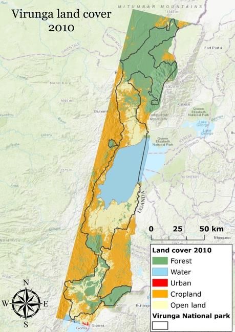
Sustainability 2020, 12, 1570                                                                        9 of 28

3.2.3. Modelling Transition Potential—MLP Calibration
      Artificial neural networks are types of computational frameworks for a collection of units or nodes
(also called neurons or perceptrons), which aim to mimic the human brain [19]. In this study, an MLP
neural network was trained in order to model the nonlinear relationships between land cover change
and the explanatory variables, thus deriving the transition potential for each type of land cover change.
Operationally, within the LCM, MLP creates a random sample of cells that transitioned and a sample
of cells that persisted and use half of the samples to train the model and develop multivariate functions
(adjusting the weights) to predict the potential for change based on the value of the conditions at each
location [15]. The other half of the subset sample of cells that transitioned and persisted is used to test
the performance of the model (validation).
      The 12 major transitions which occurred in the period between 2010 and 2015 were grouped together
in 6 different submodels, namely; Abandonment/reclamation, Afforestation, Agricultural intensification,
Deforestation, Natural dynamics and Urban intensification. The next step in modelling the transition
potential was to assign the explanatory variables to each submodel. Variables can be added to the model
either as static, meaning that they do not change over time, such as slope, or dynamic, meaning that they
do change over time, such as proximity to roads (assuming dynamic road development). Static variables
are unchanging over time and express aspects of basic suitability for transitions under consideration,
while dynamic variables are time-dependent, such as proximity to existing forest areas or road networks,
and are recalculated during the course of a future land cover simulation [13]. In this study DEM, slope,
aspect, EL, D_am, D_mining and D_water was used as static variables, while D_disturb, D_cities.
D_forests and D_roads were designated as dynamic variables. In contrast to the other distance-related
variables, D_am and D_mining are defined as static, under the assumption that the geographic location
of the mining operations remain fixed and are not expanding over time.
      An iterative approach was used to establish the most appropriate, and accurate, combination of
driver variables for each submodel, while avoiding overfitting. Each submodel was fitted with all
11 explanatory drivers to being with, and an iterative approach was used to remove the driver with
the least explanatory potential, while assessing the accuracy score and skill level of the model after
each iteration. The accuracy score provides a value in percentage that indicates how well the model is
able to predict the changes that happened between 2010 and 2015, accounting for both change and
persistence. The skill measure compares the number of correct predictions, minus those attributable to
random guessing, to that of a hypothetical perfect prediction [10]. Thus, the skill measure provides
an indication of how the explanatory drivers will explain past changes. The skill is measured on a
scale from −1 to 1, where values less than 0 indicates that the model performs worse than what would
be expected by random guessing, 0 indicates that the model performs as well as random guessing
while values between 0 and 1 indicates that the performance of the model exceeds what is expected by
pure chance.
      After each iteration of calibrating individual submodels using MLP, a report about the nature
of the model performance is created. This provides critical information on the overall accuracy and
skill of the model, the skill measure broken down by component (transition and persistence type)
and the explanatory power of each variable. In step 1, the variable with the lowest negative effect on
the skill is held constant, and this provides information on the explanatory potential of this variable.
If the accuracy and skill of the model don’t decrease by much, when holding the variable constant,
this suggests that the variable has little value and can be removed [13]. On each iteration of the
calibration of each submodel, the variable with the least explanatory potential was removed until
a combination of 5-6 of the variables with the strongest explanatory potential was left under each
submodel. Consequently, the final selected variables were loaded into the submodel structure to
execute the final iteration of the MLP training.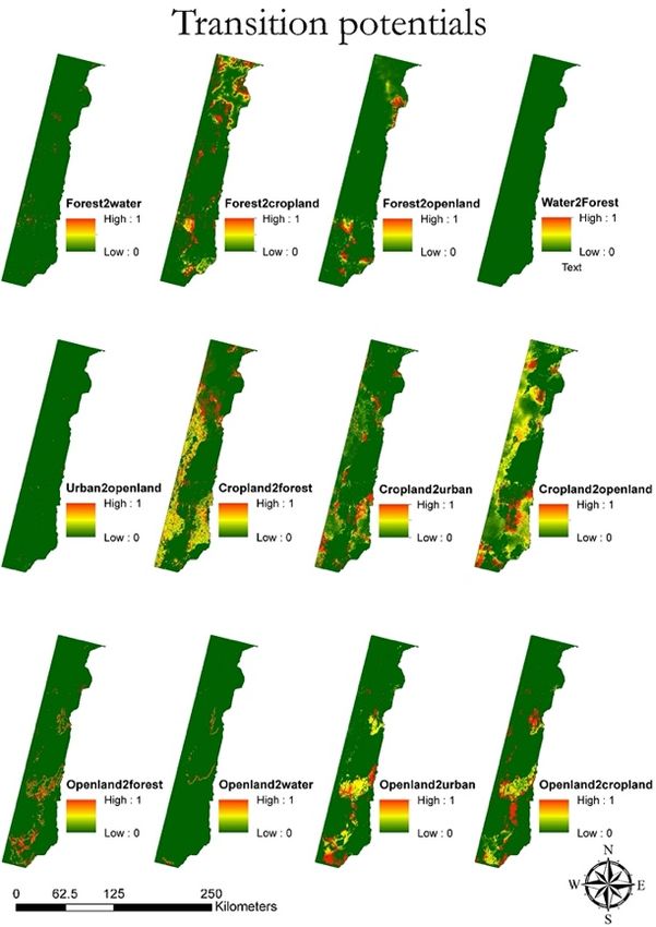
Sustainability 2020, 12, 1570                                                                      10 of 28

3.2.4. Change Prediction and Model Validation
     Following the transition submodel development, the 12 transition potential maps were used
as input in a Markov chain model to simulate future LULC changes (Table 3). The Markov chain
determines the amount of change using the earlier and later land cover map along with a pre-specified
future year [13]. The Markov module produces a transition probability matrix, which is a matrix that
records the probability of each land cover class to change into every other land class category. It also
creates a transition areas matrix which is a record of the number of pixels that are expected to change
from each land cover class over the specified time frame [13]. Finally, the Markov chain creates a set of
conditional probability images which reports the probability of a land cover type to be found at each
pixel after the specified prediction date [13]. However, as the matrices only determine the quantity of
change, the transition potential (suitability) maps are utilized within the Markov analysis to spatially
allocate changes in order to make a land cover prediction for a future year [13].

                                   Table 3. Markov chain transition probability matrix.

                         Given:                       Probability of Changing to:
                                        Forest     Water      Urban      Cropland     Open Land
                          Forest        0.3169     0.0017     0.0014      0.6271          0.0528
                          Water         0.019      0.9953     0.0000      0.0017          0.0011
                          Urban         0.0208     0.0016     0.4025      0.2786          0.2965
                        Cropland        0.1029     0.0005     0.0035      0.8022          0.0910
                       Open land        0.0701     0.0035     0.0268      0.6451          0.2545

      Consequently, Markov chain analysis was used to make a LULC prediction for 2019 and
subsequently validated by using the actual 2019 land cover map for comparison. Yearly recalculation
stages were assigned in the model to specify the frequency of which the dynamic variables are
recalculated in the model. This means that the D_disturb, D_cities. D_forests and D_roads explanatory
variables are updated in the model every year until the prediction year.
      Besides visually inspecting how the predicted land cover compare with the actual 2019 land cover
map, different Kappa Index of Agreement (KIA) scores was used to assess the overall accuracy of
the prediction. The KIA scores can be used to test the agreement between a ‘comparison’ map and a
‘reference map’, both in terms of the quantity of cells in each land cover category and the agreement
in terms of location of these cells [13]. The Kappa Standard (Kstandard) is equivalent to kappa and
indicates the proportion of correctly assigned pixels versus the proportion that is correct by chance.
The Kappa for no information (Kno) indicates the overall agreement between the simulated and
reference map [13]. The Kappa for location (Klocation) is a measure of the spatial accuracy in the
overall landscape, due to the correct assignment of values in each category between the simulated
and reference map [13]. The Kappa for stratum-level location (KlocationStrata) is a measure of the
spatial accuracy within preidentified strata, and it indicates how well the grid cells are located within
the strata. The combination of Kstandard, Kno, Klocation and KlocationStrata scores allows for a
comprehensive assessment of the overall accuracy both in terms of location and quantity. All KIA
scores range from 0 to 1 (or 0% to 100%), where 0 indicates that agreement is equal to agreement due to
chance and 1 (or 100%) indicates perfect agreement.

4. Results

4.1. Land Cover Classification
    Using the workflow described in Section 3.1, the three land cover maps for 2010, 2015 and 2019 was
generated, using Landsat data. The resulting land cover classifications can be seen in Figure 3 below.
Sustainability 2020, 12, 1570 11 of 28
Sustainability 2020, 11, x FOR PEER REVIEW 12 of 31
Figure 3. Generated land cover maps.
The overall accuracy, producers- and users’ accuracy for each of the three land cover maps can
be seen in Table 4, and the quantified land
Figure
Figure cover area
Generated
3.Generated
3. land under
landcover each land class, and for each year, can
covermaps.
maps.
be seen fromThe
theoverall
graphaccuracy,
presented in Figure 4.
producers- and users’ accuracy for each of the three land cover maps can be
The overall accuracy, producers‐ and users’ accuracy for each of the three land cover maps can
seen in Table
be seen 4, and
in Table the quantified
4, and landland
the quantified covercover
area area
under each each
under land land
class,class,
and for
andeach
for year, can becan
each year, seen
from the Table
graph 4. Accuracy
presented in scores
Figure 4. for the 2010, 2015 and 2019 land cover maps.
be seen from the graph presented in Figure 4.
Overall
Table 4.
Table AccuracyAccuracy
4. Accuracy scoresfor
scores forthe Producer’s
the2010,
2010, 2015and
2015
Accuracy
and2019Accuracy
2019 landcover
land
User’s
covermaps.
maps.
Land Cover Class 2010 2015 2019 2010 2015 2019 2010 2015 2019
Overall Accuracy
Overall Producer’sAccuracy
Accuracy Producer’s Accuracy User’sUser’s Accuracy
Accuracy
Forest 96 90.9 100 96 100 86
LandLand
CoverCover
Class Class
2010 20102015
2015 2019
2019 2010
2010 2015
2015 2019 2019 201020102015 2015
2019 2019
Water
ForestForest
100 90.9
96
96
100 100
90.9
100 100
100 96 96 100 10086
100 86 100
Urban
WaterWater 95.5 100
100
100 97.8 100
100 10097.9 84 100100
100100 100 90 100 92
Urban
Cropland Urban 95.5
95.5
91.8 97.8
97.8
100 97.9
97.9 8084 84 90
90 90 9282 92 88
Cropland
Cropland 91.8
91.8 100
100 8080 90 90 82 8288 88
Open
OpenLand
Land 82.5 84.5
82.5 84.5 85.585.5 94 94 98 98 94 94
Open Land 82.5 84.5 85.5 94 98 94
Total(in
Total (in %)
%) 92.8 94 92 93.2 94.6 92.792.7 92.892.8 94 94 92 92
Total (in %) 92.892.8 9494 92
92 93.2 94.6
93.2 94.692.7 92.8 94 92
AreaArea
underunder eachland
each landcover
cover class
classin in
2010, 20152015
2010, and 2019
and 2019
8000
8000 7000
7000 6000
Area (km2)
6000 5000
Area (km2)
4000
5000
3000
4000 2000
3000 1000
2000 0
Forest Water Urban Cropland Open land
1000 2010 5113 1773 18 4538 3035
0 2015 3646 1780 76 6878 2098
Forest Water Urban Cropland Open land
2019 3358 1767 69 7105 2154
2010 5113 1773 18 4538 3035
2015 3646 4. Land cover
Figure 1780area per class 76 6878
in 2010, 2015 and 2019. 2098
2019 3358 1767 69 7105 2154
Land Changes
In order to assess the spatiotemporal changes between 2010 and 2015, the earlier and latter land
Figure 4. Land
Figure cover
4. Land area
cover areaper classinin2010,
per class 2010, 2015
2015 andand
2019.2019.
cover maps were cross‐tabulated. The cross‐tabulation table shown in Table 5 shows the frequencies
Land Changes
In order to assess the spatiotemporal changes between 2010 and 2015, the earlier and latter land
cover maps were cross-tabulated. The cross-tabulation table shown in Table 5 shows the frequenciesSustainability 2020, 12, 1570 12 of 28
Land Changes
In order to assess the spatiotemporal changes between 2010 and 2015, the earlier and latter land
cover maps were cross-tabulated. The cross-tabulation table shown in Table 5 shows the frequencies
with which the land classes remained the same (Diagonal) or changed into other categories (off-diagonal
frequencies). The table represents quantities of conversion from the earlier to the later land cover
data, and it clearly depicts significant changes, primarily between forest and cropland. The following
information was obtained about the changes in each class from the table:
1. Between 2010 and 2015 the forest cover was reduced by 28.7% from 5113.4 km2 in 2010 to 3646.4 km2
in 2015. Even though there was a forest gain of 318.9 km2 largely caused by afforestation from
cropland and open land, the net loss of 1467 km2 is almost exclusively attributed to forest
conversion into cropland.
2. Accounting for the least prevalent land class in the case study area, urban areas have experienced
a large increase between 2010 and 2015, from 17.8 km2 to 75.6 km2 , resulting in a 57.9 km2 net
gain. This is largely attributed with rapid urbanisation processes in the Democratic Republic
of Congo in general, which has an estimated average annual urban population growth rate of
4.3% [20]. The population of the capital city in the North Kivu province, Goma, located in the
south-eastern corner of the case study area, increased from 150,000 people in 1990 to more than
one million in 2017 [6]. Thus, the majority of the urban class increase is caused by the expansion
of Goma.
3. Cropland is the most dynamic land class in the case study area and represents the most dominant
land cover type. The total area under cultivation increased by 51.5%, from 4538.4 km2 in 2010 to
6877.6 km2 in 2015. As mentioned previously, cropland is the main driver of deforestation and thus
the majority of the agricultural expansion is caused by forest conversion. However, another 47%
of cropland expansion is attributed with the cultivation of previously open land/grassland areas.
4. The open land cover class was reduced by 30.8%, from 3035.0 km2 in 2010 to 2098.3 km2 in
2015. Even though the open land class received a total net loss, 236.2 km2 was gained, caused by
agricultural abandonment. Another 66 km2 gain of open land is attributed to deforestation.
The majority of the net loss of the open land class (1109.2 km2 ) is associated with agricultural
expansion, while another 59,5 km2 is attributed to urbanisation processes. A net loss of 69.8 km2
is associated with afforestation processes.
5. The water bodies remained largely unchanged, which is to be expected as there has been no
waterworks (e.g., dam construction) in the study period. Thus, the water bodies, largely consisting
from the two major lakes in the study area, Lake Édouard and Lake Kivu, have remained
relatively consistent.
Table 5. LULC change matrix for the period from 2010 to 2015 (km2 ) class.
LC_2010
Land Class Forest Water Urban Cropland Open Land Total (km2 )
Forest 3327.5 1.6 0.0 247.5 69.8 3646.4
Water 3.8 1770.2 0.0 0.3 5.2 1779.5
Urban 0.6 0.0 13.0 2.5 59.5 75.6
Cropland 1715.4 0.3 0.9 4051.8 1109.2 6877.6
LC_2015
Open land 66.1 0.9 3.8 236.2 1791.2 2098.3
Total (km2 ) 5113.4 1773.0 17.8 4538.4 3035.0 14,477.5
The spatial trends of the changes outlined above are illustrated in Figure 5 below.
4.2. LULC Model
Using the 2010 and 2015 land cover maps and the explanatory variables as input data, the model
described in the methods section was trained to make a land cover prediction for each year betweenSustainability 2020, 12, 1570 13 of 28
2020 and 2030. Table 6 provides a list of the Cramer’s V scores of each explanatory variable used in the
model and Figure 6 illustrates all the processed variables.
Sustainability 2020, 11, x FOR PEER REVIEW 14 of 31
Figure 5. Class transitions between 2010 and 2015.
Figure 5. Class transitions between 2010 and 2015.
Sustainability 2020, 11, x FOR PEER REVIEW 16 of 31
4.2. LULC Model
Using the 2010 and 2015 land cover maps and the explanatory variables as input data, the model
described in the methods section was trained to make a land cover prediction for each year between
2020 and 2030. Table 6 provides a list of the Cramer’s V scores of each explanatory variable used in
the model and Figure 6 illustrates all the processed variables.
Figure 6. Processed explanatory variable datasets used as input for the MLP modelling.
Figure 6. Processed explanatory variable datasets used as input for the MLP modelling.
Table 7 below provides information on the accuracy and skill measure of the model when
holding one or more variables constant. This relationship was used to identify the explanatory
variables with the strongest explanation potential for each transition type.Sustainability 2020, 12, 1570 14 of 28
Table 6. Cramer’s V scores for each of the explanatory variables.
Variable DEM Asp Slope EL D_am D_disturb D_cities D_forests D_mining D_roads D_water
Forest 0.52 0.21 0.26 0.68 0.17 0.40 0.17 0.43 0.14 0.26 0.27
Water 0.61 0.83 0.57 0.42 0.32 0.68 0.54 0.82 0.27 0.57 0.30
Cramer’s V Urban 0.14 0.07 0.06 0.10 0.08 0.04 0.06 0.04 0.09 0.09 0.07
Cropland 0.42 0.32 0.34 0.29 0.31 0.52 0.20 0.32 0.31 0.34 0.29
Open land 0.23 0.17 0.24 0.65 0.20 0.15 0.18 0.30 0.24 0.11 0.08
Overall 0.42 0.42 0.33 0.48 0.22 0.42 0.28 0.46 0.22 0.32 0.20Sustainability 2020, 12, 1570 15 of 28
Table 7 below provides information on the accuracy and skill measure of the model when holding
one or more variables constant. This relationship was used to identify the explanatory variables with
the strongest explanation potential for each transition type.
Sustainability 2020, 11, x FOR PEER REVIEW 17 of 31
Table 7. Extract
Table from
7. Extract thethe
from calibration
calibrationreport indicatingaccuracy
report indicating accuracy scores
scores andand
skillskill measure
measure of theofmodel
the model
when holding
when variables
holding variablesconstant.
constant.
Backwards Stepwise Constant Forcing Forcing
Model Variables Included
Variables Included Accuracy
Accuracy(%)
(%) Skill Measure
Skill
With
With all
all variables
variables Allvariables
All variables 72.25
72.25 0.6300
0.6300
Step 1: var.[5] constant
Step 1: var.[5] constant [1,2,3,4,6,7,8,9,10]
[1,2,3,4,6,7,8,9,10] 72.25
72.25 0.6300
0.6300
Step 2: var.[5,10] constant [1,2,3,4,6,7,8,9] 72.23 0.6298
Step 2: var.[5,10] constant [1,2,3,4,6,7,8,9] 72.23 0.6298
Step 3: var.[5,10,7] constant [1,2,3,4,6,8,9] 72.06 0.6275
Step 3: var.[5,10,7] constant [1,2,3,4,6,8,9] 72.06 0.6275
Step 4: var.[5,10,7,9] constant [1,2,3,4,6,8] 69.86 0.5981
Step 5:
Step 4: var.[5,10,7,9]
var.[5,10,7,9,4]constant
constant [1,2,3,4,6,8]
[1,2,3,6,8] 69.86
65.48 0.5981
0.5397
Step 6: var.[5,10,7,9,4,8]constant
Step 5: var.[5,10,7,9,4] constant [1,2,3,6,8]
[1,2,3,6] 65.48
62.59 0.5397
0.4999
Step 7:
Step 6: var.[5,10,7,9,4,8]
var.[5,10,7,9,4,8,3]constant
constant [1,2,3,6]
[1,2,6] 62.59
54.55 0.4999
0.3940
7: var.[5,10,7,9,4,8,3]
Step 8: var.[5,10,7,9,4,8,3,1]constant
constant [1,2,6]
[2,6] 54.55
47.77 0.3940
0.3036
8: var.[5,10,7,9,4,8,3,1]
Step 9: var.[5,10,7,9,4,8,3,1,6]constant
constant [2,6]
[2] 47.77
29.40 0.3036
0.0587
Step 9: var.[5,10,7,9,4,8,3,1,6] constant [2] 29.40 0.0587
The final skill measure and accuracy rate of each model calculated through MLP is summarized
The final skill measure and accuracy rate of each model calculated through MLP is summarized
in Figure 7 and the explanatory drivers used under each submodel and selected performance scores is
in Figure 7 and the explanatory drivers used under each submodel and selected performance scores
provided in Table
is provided 8. 8.
in Table
Figure7.7.Submodel
Figure Submodel accuracy
accuracyand
andskill measure
skill from
measure MLP.
from MLP.
TheThe accuracyand
accuracy andskill
skill measure
measure reveal
revealsome
somedisparity between
disparity the level
between theoflevel
confidence of the
of confidence of
transition modelling under each submodel, however overall the values are fairly
the transition modelling under each submodel, however overall the values are fairly consistent,consistent, ranging
from 75% to 93%. Abandonment/reclamation has the lowest accuracy score (75.12%), followed by
ranging from 75% to 93%. Abandonment/reclamation has the lowest accuracy score (75.12%),
deforestation (77.61%), afforestation (77.79%) and agricultural intensification (78.23%). Agricultural
followed by deforestation (77.61%), afforestation (77.79%) and agricultural intensification (78.23%).
intensification, however, has the lowest skill measure of all the submodels (0.56). Natural dynamics
Agricultural intensification, however, has the lowest skill measure of all the submodels (0.56).
and urban intensification performed best, with accuracies of 93.90% and 83.41%, respectively. The
Natural
skill dynamics
measure ofand urban
these intensification
two submodels was performed best,among
also the highest with accuracies
all six, withof0.93
93.90% and 83.41%,
for natural
respectively.
dynamicsThe andskill
0.78 measure
for urbanof these two submodels
intensification. The outcomewasofalso
thethe highestpotential
transition among all six, with
modelling is 0.93
a for
natural dynamics and 0.78 for urban intensification. The outcome of the transition potential
series of transition potential maps, describing the suitability for each of the 12 major transitions modelling
is a series
includedof in
transition potential
the submodels. maps,
These mapsdescribing
can be seenthe suitability
in Figure 8. for each of the 12 major transitions
included in the submodels. These maps can be seen in Figure 8.Sustainability 2020, 12, 1570 16 of 28
Table 8. Submodels included in MLP with associated explanatory variables and selected performance indicators.
RMS
Submodel Explanatory Variables Transition/Persistence Class Class Skill Measure (ratio) Submodel Accuracy Submodel Skill
Training Testing
Urban to Openland 0.8134
Cropland to Openland 0.5741
Abandonment/reclamation DEM; Slope; D_am; D_cities; D_mining; D_water 75.12% 0.6682 0.2980 0.3071
Persistence: Urban 0.7401
Persistence: Cropland 0.5398
Cropland to Forest 0.5181
Openland to Forest 0.8918
Afforestation DEM; Slope; EL; D_disturb; D_forests; D_water 77.79% 0.7038 0.2751 0.2737
Persistence: Cropland 0.6536
Persistence: Openland 0.7515
Openland to Cropland 0.5961
Agricultural intensification DEM; D_am; D_disturb; D_mining; D_roads; D_water 78.23% 0.5646 0.3899 0.3906
Persistence: Openland 0.5329
Forest to Cropland 0.6103
Deforestation DEM; D_am; D_disturb; D_mining; D_roads; D_water Forest to Openland 0.8300 77.61% 0.6642 0.3358 0.3369
Persistence: Forest 0.5516
Forest to Water 0.9848
Water to Forest 0.9096
Openland to Water 0.8707
Natural dynamics DEM; Slope; EL; D_forests; D_water 93.90% 0.9269 0.1207 0.1281
Persistence: Forest 0.8677
Persistence: Water 0.9849
Persistence: Openland 0.9441
Cropland to Urban 0.8664
Openland to Urban 0.6564
Urban intensification Slope; EL; D_am; D_cities; D_mining; D_roads 83.41% 0.7788 0.2536 0.2489
Persistence: Cropland 0.8294
Persistence: Openland 0.7630Sustainability2020,
Sustainability 2020,12,
12,1570
x FOR PEER REVIEW 1 of 28
17 31
Figure 8.
Figure 8. Transition
Transition potentials.
potentials.
4.2.1.
4.2.1. Validating
Validating Results
Results
Figure
Figure99below
belowshows
showsthetheactual
actualand
andthe
thepredicted
predictedlandlandcover
covermap
mapforfor2019.
2019. The
The actual
actual 2019
2019 land
land
cover map was created using Landsat data composites from the years 2017–2019,
cover map was created using Landsat data composites from the years 2017–2019, applying the applying the process
described in Section
process described in3.1.3. A visual
Section 3.1.3. Ainspection indicatesindicates
visual inspection that the that
predicted land cover
the predicted landmap, overall,
cover map,
looks fairly
overall, similar
looks fairlyto the actual
similar to theland cover
actual landmap,
coverhowever there are
map, however localised
there discrepancies
are localised where
discrepancies
the model
where thefailed
modelto failed
predicttochanges/persistence, for example,
predict changes/persistence, for in the mid-west
example, in thewhere the simulation
mid‐west where the
predicted
simulationcropland
predicted to cropland
replace large open land
to replace largeareas,
openwhen in actuality
land areas, when itindid not. it did not.
actuality
K scores was used to comprehensively assess how the simulated 2019 land cover map ‘comparison’
compare with the actual 2019 land cover map ‘reference’. The K scores are provided in Table 9.
Table 9. K scores for 2019.
K INDICATORS 2019
KSTANDARD 0.8828
KNO 0.9224
KLOCATION 0.9001
KLOCATIONSTRATA 0.9001
The statistics from the k scores shows that Kno is 0.9224, Klocation is 0.9001, KlocationStrata is 0.9001
and the overall Kstandard is 0.8828. According to [21], a model is valid if the overall Kappa (Kstandard )Sustainability 2020, 12, 1570 18 of 28
score exceeds 70% (or 0.7). The Kstandard score, close to 90%, is a very strong indicator of the overall
accuracy and performance of the model, and the remaining k scores, all exceeding 85%, indicate that
there are almost no, or very small quantification and location errors between the predicted and the
actual land cover map for 2019. Thus, the simulation has a strong ability to predict both the quantity
Sustainability 2020, 12, of
and the locations x FOR PEER REVIEW
change. 2 of 31
Figure 9.
Figure Actualland
9. Actual land cover
cover map
map for
for 2019
2019 versus
versus the
the predicted
predicted 2019
2019 land
land cover
cover map.
map.
4.2.2. Land Cover Prediction
K scores was used to comprehensively assess how the simulated 2019 land cover map
The resulting
‘comparison’ compare compilation of land2019
with the actual cover predictions
land cover mapfrom 2020 through
‘reference’. The Ktoscores
2030 can
are be seen from
provided in
Sustainability 2020, 12, x FOR PEER REVIEW 3 of 31
Figure9.10, while the predicted land cover for 2030 is presented in Figure 11.
Table
Table 9. K scores for 2019.
K INDICATORS 2019
KSTANDARD 0.8828
KNO 0.9224
KLOCATION 0.9001
KLOCATIONSTRATA 0.9001
The statistics from the k scores shows that Kno is 0.9224, Klocation is 0.9001, KlocationStrata is 0.9001 and
the overall Kstandard is 0.8828. According to [21], a model is valid if the overall Kappa (Kstandard) score
exceeds 70% (or 0.7). The Kstandard score, close to 90%, is a very strong indicator of the overall accuracy
and performance of the model, and the remaining k scores, all exceeding 85%, indicate that there are
almost no, or very small quantification and location errors between the predicted and the actual land
cover map for 2019. Thus, the simulation has a strong ability to predict both the quantity and the
locations of change.
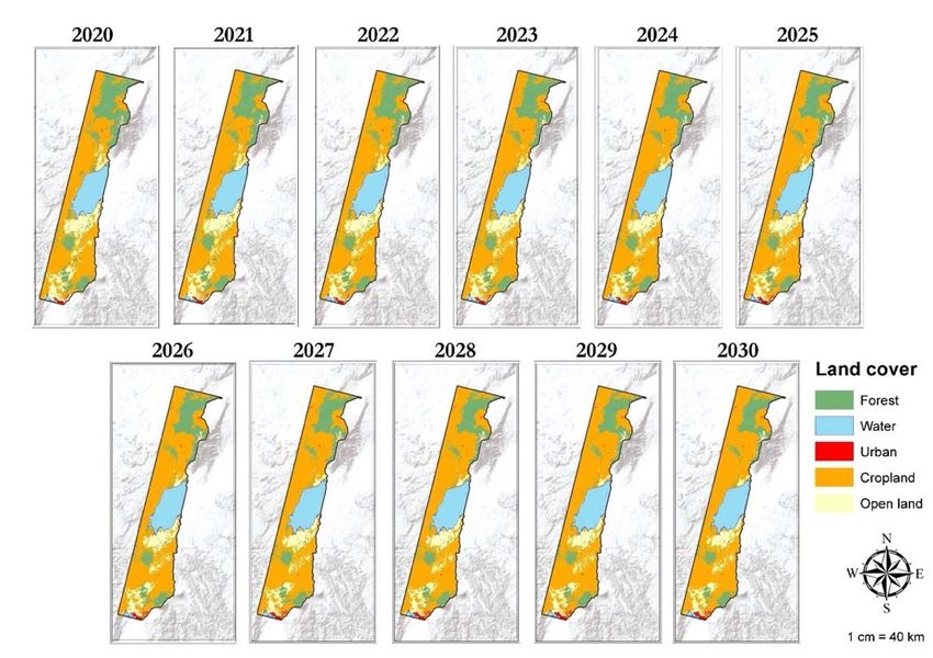
4.2.2. Land Cover Prediction
The resulting compilation of land cover predictions from 2020 through to 2030 can be seen from
Figure 10, while the predicted land cover for 2030 is presented in Figure 11.
Figure 10. Predicted land cover maps from 2020 to 2030.
Figure 10. Predicted land cover maps from 2020 to 2030.Sustainability 2020, 12, 1570 19 of 28
Figure 10. Predicted land cover maps from 2020 to 2030.
Figure 11. Predicted
Figure 11. Predicted2030 landcover
2030 land cover in Virunga.
in Virunga.
The series of land cover predictions covering 2020 to 2030, and the final land cover map for
The series of land cover
2030 presented predictions
in Figure covering
11 clearly illustrates 2020
that the to 2030,
model predictsand the final
continuous landexpansion,
cropland cover map for 2030
presented in Figureat the
primarily 11 expense
clearlyofillustrates that
forest areas and the model
existing predicts
open lands. The modelcontinuous
also predicts cropland
continuous expansion,
urban development, particularly around existing settlements. The collective change per class in
primarily at the expense of forest areas and existing open lands. The model also predicts continuous
total, and percent change per year, is illustrated in Figure 12. As depicted in the graph, the forest
urban development, particularly
cover will continue around
to decrease existing
throughout settlements.
the 10-year The
period, with ancollective change
average annual loss ofper class in total,
4.21%
and percentand
change
a total per
area year,
loss of is illustrated
1085 km , from in
2 Figure
3104 km in 12.
2 2020As depicted
to 2019 km inin
2 theWater
2030. graph, the forest
coverage will, cover will
as expected, remain largely the same, gaining a negligible average of 0.04% per year. Urban expansion
and development of new settlements will continue, gaining an average annual of 3.44%. The total
urban area is predicted to increase by 38 km2 , from 95 km2 in 2020 to 133 km2 in 2030, and looking
at the predicted land cover map, most of this is expected to be as a result of urban sprawl around
the main city of Goma in south-eastern Virunga. As also visually apparent, cropland expansion will
continue throughout the 10-year period, gaining an average annual area of 1.83%, and a total area gain
of 1522 km2 , from 7636 km2 to 9161 km2 class coverage. Along with forest areas, open land/grassland
zones are expected to decrease the most, by 2.96% per year, losing a total of 482 km2 in the 10-year
period, from 1857 km2 in 2020 to 1375 km2 in 2030.area is predicted to increase by 38 km2, from 95 km2 in 2020 to 133 km2 in 2030, and looking at the
predicted land cover map, most of this is expected to be as a result of urban sprawl around the main
city of Goma in south‐eastern Virunga. As also visually apparent, cropland expansion will continue
throughout the 10‐year period, gaining an average annual area of 1.83%, and a total area gain of 1522
km2, from 7636 km2 to 9161 km2 class coverage. Along with forest areas, open land/grassland zones
Sustainability 2020, 12,to1570
are expected 20 of 28
decrease the most, by 2.96% per year, losing a total of 482 km2 in the 10‐year period,
from 1857 km in 2020 to 1375 km in 2030.
2 2
Land cover change 2020 ‐ 2030
9,500
8,500 4
7,500
2
% gain/loss per year
6,500
Km2 per class
5,500
0
4,500
3,500
‐2
2,500
1,500 ‐4
500
‐500 2020 2021 2022 2023 2024 2025 2026 2027 2028 2029 2030 ‐6
Forest Water Urban Cropland Open land
Forest Water Urban Cropland Open land
Figure
Figure 12. Predicted
12. Predicted landland cover
cover (km 2 ) 2for
(km ) foreach
eachland
landcover
cover class
class for
for each
eachyear
yearbetween
between2020–2030
2020–2030 and
and %
% yearly (gain/loss) per class. The horizontal lines indicate the yearly gain/loss in percent for
yearly (gain/loss) per class. The horizontal lines indicate the yearly gain/loss in percent for each class, each
whileclass, while the columns indicate the total land cover 2in km2 for each class for each year.
the columns indicate the total land cover in km for each class for each year.
5. Discussion
5. Discussion
Understanding LULC changes, transitions, landscape risks and dynamics is paramount in order
Understanding LULC changes, transitions, landscape risks and dynamics is paramount in order
to inform policies, planning interventions and actions aiming to ensure sustainable development in
to inform policies, planning interventions and actions aiming to ensure sustainable development in
all dimensions (economic, social and environmental) conforming to the objective of the UN SDG’s
all dimensions (economic, social and environmental) conforming to the objective of the UN SDG’s
and the 2030 agenda for sustainable development. In this study, a combined MLP‐Markov chain
and the
approach has beenfor
2030 agenda usedsustainable
to simulate development.
future land coverInchanges
this study,
in theaperiod
combined MLP-Markov
from 2020 to 2030, in achain
approach has been
case study used to simulate
area covering the Virungafuture
NP inland cover changes
the Democratic in the
Republic period
of the Congo from
and 2020 to 2030, in a
its immediate
case study area
vicinity. covering
Two the Virunga
simulations NP inout.
were carried theThe
Democratic Republic
first (2019) was usedof the
for Congo and its immediate
model validation and
accuracy
vicinity. assessment, and
Two simulations werethe second
carried (2030)
out. Thewas
firstused to was
(2019) predict
usedlandscape change
for model within and
validation the case
accuracy
study area
assessment, andcovering the Virunga
the second NP used
(2030) was catchment. The assessment
to predict landscape of the spatial
change within patterns
the case of study
LULC area
covering the Virunga NP catchment. The assessment of the spatial patterns of LULC changeof
change derived through a change analysis of historical trends combined with the development a
derived
plausible future land cover scenario for the Virunga catchment will help to improve the
through a change analysis of historical trends combined with the development of a plausible future
understanding of the land system and establish cause‐effect relationships between driver variables
land cover scenario for the Virunga catchment will help to improve the understanding of the land
and land cover dynamics. Thus, the LULC change model aims to contribute to informing policy
system and establish cause-effect relationships between driver variables and land cover dynamics.
Thus, the LULC change model aims to contribute to informing policy responses aiming to support
sustainable land management and landscape planning decisions within the Virunga NP. It aims to
provide a blueprint for quantified policy responses aiming to address existing challenges. Follow-up
research should aim at applying the LULC model developed for this study for scenario-based analysis
of policy response impacts.
As formerly mentioned, the LULC model developed in this study predicts a future land cover
state, based on a business as usual scenario. Past land cover changes within the Virunga catchment
has been largely linked with charcoal production and cropland expansion, which have impeded
conservation efforts and put critical pressure on the ecological integrity of the landscape and its
biodiversity. By cross-tabulating two land cover maps for 2010 and 2015, this study aimed to quantify
past land cover changes and identify spatial trends of change. It concludes that forest conversion into
cropland is the most common and frequent type of landcover change, contributing to the majority of the
total net forest loss of 28.7% between 2010 and 2015. The most significant forest loss occurred aroundYou can also read