A stochastic individual based model for the growth of a stand of Japanese knotweed including mowing as a management technique.
←
→
Page content transcription
If your browser does not render page correctly, please read the page content below
A stochastic individual based model for the growth of a stand of Japanese knotweed
including mowing as a management technique.
François Lavallée1,2,∗, Charline Smadi1,2 , Isabelle Alvarez1,2 , Björn Reineking3 , François-Marie Martin3 , Fanny Dommanget3 ,
Sophie Martin1,2 ,
Abstract
Invasive alien species are a growing threat for environment and health. They also have a major economic impact, as they can
arXiv:1902.06971v1 [q-bio.PE] 19 Feb 2019
damage many infrastructures. The Japanese knotweed (Fallopia japonica), present in North America, Northern and Central Europe
as well as in Australia and New Zealand, is listed by the World Conservation Union as one of the world’s worst invasive species.
So far, most models have dealt with how the invasion spreads without management. This paper aims at providing a model able
to study and predict the dynamics of a stand of Japanese knotweed taking into account mowing as a management technique. The
model we propose is stochastic and individual-based, which allows us taking into account the behaviour of individuals depending
on their size and location, as well as individual stochasticity. We set plant dynamics parameters thanks to a calibration with field
data, and study the influence of the initial population size, the mean number of mowing events a year and the management project
duration on mean area and mean number of crowns of stands. In particular, our results provide the sets of parameters for which it
is possible to obtain the stand eradication, and the minimal duration of the management project necessary to achieve this latter.
Keywords: Invasive plant, Fallopia spp., Reynoutria spp., Polygonum spp., individual based model, management strategies,
dynamics, model exploration
1. Introduction bringing the density of the invasive species below a threshold.
For seed dispersal species, a frequent question in the literature
Invasive alien species are a growing problem for environment
of invasive species through mathematical modelling is to assess
and health. They may cause a loss of biodiversity (Murphy and
the benefit of a spatial prioritization: is it more profitable to re-
Romanuk, 2014), changes in ecosystem functioning (Strayer,
move the individuals at the heart of the infection, or those on
2012) or affect human well-being (Shackleton et al., 2019).
the periphery (Harris et al., 2009) ? The answer depends es-
They also have a major economic impact (Kettunen et al., 2008;
sentially on the spatial spread of the plant (and therefore on the
Pimentel et al., 2005). The necessity to act against invasive
species considered). Another issue in the literature of invasive
species relies on their global and local impacts and also on in-
species management is the temporal distribution of the effort: is
ternational policy engagements. For example, since 1992, the
it better to act significantly at the beginning of the management
Convention on Biological Diversity (article 84 ) compels the par-
project and then to control the invasion with a lower effort (as
ties to "prevent the introduction of, control or eradicate those
in Meier et al. (2014)), or to increase the effort over time (as in
alien species which threaten ecosystems, habitats or species".
Baker and Bode (2016))? A common assumption when dealing
Invasive species management raises several issues and strate-
with control strategies is that the invasive species has already
gies depend on the species, the step reached on the invasion
been present for a long time (Baker and Bode, 2016). We know
process and the scale of action (Simberloff et al., 2013).
however that early detection and rapid response to the invasion
Together with field experiments, mathematical models can
may have a greater efficiency (Pyšek and Richardson, 2010).
provide a better understanding of the critical determinants of
Among the worst invasive species threatening biodiversity,
the growth and spread of these species and thus help to identify
Asian knotweeds raise particular management issues. This
efficient management strategies. Many studies focus on optimal
complex of three species (the Japanese knotweed, Fallopia
management of invasive species (Baker and Bode, 2016; Har-
japonica [Houtt.] Ronse Decraene, the giant knotweed, Fal-
ris et al., 2009; Travis et al., 2011). Control strategies aim at
lopia sachalinensis [Schmidt Petrop.] Ronse Decraene and the
∗ Corresponding author
hybrid between the two previous the Bohemian knotweed (Fal-
Email address: francois.lavallee@irstea.fr (François Lavallée) lopia × bohemica Chrtek & Chrtkova) have invaded Europe and
1 IRSTEA UR LISC, Laboratoire d’ingénierie pour les Systèmes Com-
North America. Native to Eastern Asia, knotweeds have been
plexes, 9 avenue Blaise-Pascal CS 20085, 63178 Aubière, France introduced for ornamental purpose at the end of the 19th cen-
2 Complex Systems Institute of Paris Île-de-France, 113 rue Nationale,
75013, Paris, France
tury (Bailey and Wisskirchen, 2006; Barney et al., 2006; Beer-
3 Univ. Grenoble Alpes, Irstea, LESSEM, 38000 Grenoble, France ling et al., 1994). They are also present in Australia, New
4 https://www.cbd.int/convention/articles/default.shtml?a=cbd-08 Zealand and Chile (Alberternst and Böhmer, 2006; Saldaña
Preprint submitted to Elsevier February 20, 2019et al., 2009). control of Fallopia japonica using one of its co-evolved natu-
Asian knotweeds quickly invade the environment in which ral enemies, the Japanese sap-sucking psyllid Aphalara itadori.
they grow (Gowton et al., 2016) and have large impacts (Lavoie, It is a deterministic model that describes the evolution of the
2017). They displace other plant species through light compe- number of insects (larvae and adults), the total weight of the
tition and allelopathy (Dommanget et al., 2014; Siemens and knotweed stems and the rhizome biomass. A key parameter of
Blossey, 2007), affect native fauna diversity (Abgrall et al., their model is the duration that a larva takes to consume and
2018; Gerber et al., 2008; Maerz et al., 2005; Serniak et al., digest the rhizome biomass of the plant.
2017) and modify ecosystem functioning (Dassonville et al., A commonly used management technique for Asian
2011; Tharayil et al., 2013). In addition, the control costs are knotweed stands is mowing. Managers can vary its intensity
very high and were estimated at 250 million dollars a year in and frequency, which motivates a study of the effects of these
Great Britain (Colleran and Goodall, 2014) and more than 2 two parameters on the dynamics of the stand. This paper aims at
billion euros a year in Europe (Kettunen et al., 2009). understanding the influence of mowing on the growth of a Asian
Asian knotweeds grow in a wide variety of soils: sandy, knotweed stand. More precisely, we study the influence of the
swampy, rocky. They mainly invade human modified habitats initial population size, the mean number of mowing events a
such as roadsides, waste dumps, but also river banks. They year and the management project duration on mean area and
are perennial geophytes: their rhizomes allow them to spend mean number of crowns of the stands. To our knowledge, exist-
the winter season buried in the ground (De Waal, 2001). Their ing models are not well designed to study such questions. Here
rhizomes also play a major role in their propagation, thanks to we present a stochastic individual based model for the growth of
their strong regeneration capacities (Bailey et al., 2009; Brock a stand of Japanese knotweed including mowing as a manage-
et al., 1992). Once arrived in a new area, the rhizome expands ment technique. The stochastic formalism enables us to study
centrifugally and a new stand can sustainably establish in a few the early stage of invasion, without assuming the species has
weeks (Gowton et al., 2016; Smith et al., 2007). been present for a long time. The description of phenomena
Once established and due to their extensive rhizome network, at the level of individuals enables us to take into account the
Asian knotweeds are extremely hard to remove. Rhizomes variability between crowns, for example due to different ages.
represent two third of their biomass (Barney et al., 2006) and The study will focus on the influence of management parame-
can expand several meters away from the visible invasion front ters on model outputs which are area and number of crowns of
(Barney et al., 2006). The resources they store can be efficiently the stand.
remobilized after mowing events (Rouifed et al., 2011). Some The paper is organized as follows. Section 2 is devoted to the
authors estimate that six cuttings are needed to significantly re- description of the ecological mechanisms taken into account in
duce belowground biomass (Gerber et al., 2010). Understand- the model (apical dominance, intraspecific competition, etc.),
ing the underground development of Asian knotweeds is cru- the presentation of the mathematical model, as well as the meth-
cial to gain insight in their local propagation and performance. ods we used for our study. Results are given in Section 3.
Moreover it could help to better design efficient management In particular, we performed a calibration of the plant dynam-
strategies. ics with field data from stands observed in the French Alps.
As underground organs are almost inaccessible to observers, We also studied, using numerical simulations with OpenMOLE
direct observations are scarce and models could help to ap- software (Reuillon et al., 2013), the influence of management
proach their dynamics and better understand how management parameters on the population growth. Finally, we summarize
actions can affect their development. To our knowledge, there our results and discuss their implications and shortcomings in
are very few models in the literature that describe the growth Section 4.
of a Japanese knotweed stand, and among them, rare are those
that include a management technique.
In Smith et al. (2007), the authors build a 3D correlated ran- 2. Materials and methods
dom walk model of the development of the subterranean rhi-
zome network for a single stand of Japanese knotweed. Their In this section we provide a description of the dynamical
model is based on knowledge of the morphology and physiol- model for the growth of a stand of Japanese knotweed includ-
ogy of the plant. They study the model through simulations and ing mowing as a management technique. We also describe the
they observe a quadratic expansion of the area invaded. methods used to its study through numerical simulations.
Dauer and Jongejans (2013) propose an "Integral Projection In the sequel, the term individual will refer to crowns, we
Model", inspired from matrix population models, for the plant recall that a crown is the location of a terminal bud from which
dynamics at the level of a stand. The variable of interest is stems emerge. Individuals are characterized by their position x
a continuous variable which stands for the height or the total in the plane and their underground biomass a (i.e. the biomass
biomass of the plant, and the authors use a simplified plant life rhizome connected to the crown).
cycle to model transition between states, like the transition from The following notations will be needed to describe our
new shoots to crown (a crown is the location of a terminal bud model:
from which stems emerge). They study the parameters that have
the largest effect on the growth rate of the population. • χ = R2 × R+ , is the state space of positions and biomasses.
Gourley et al. (2016) develop a mathematical model for bio- In the model, a crown is represented by a Dirac mass δ(x,a) ,
2with (x, a) ∈ χ, where x stands for the position of the Dispersal of the created individual: an individual with trait
crown and a is the biomass associated with the crown. (x, a) which gives birth generates an individual at position x0 .
Here we choose a Gamma law density denoted by D for the
• The set of crowns present at time t is described by the mea- birth distance law. The parameters (shape, scale) of the law
sure Zt ∈ M(χ), where M(χ) is the set of finite point mea- will be subject to calibration. We assume a uniform distribution
sures on χ whose masses of points are 0 or 1. on x0 − x direction angle to the X-axis.
n
Moreover, we will model the phenomenon of intra-specific
X
M(χ) = δ , , . . . , , χ .
(xi ,ai ) n ≥ 0, (x 1 a1 ), (xn an ) ∈
competition by considering that an individual is really born if it
i=1
does not fall too close to an already existing crown (otherwise
we consider that it is not born). So we introduce the set C de-
• MF (χ) [resp. P(χ)] is the set of finite measures (resp. pending on the population state Z and position of the potential
probability measures) on χ, such that M(χ) ⊂ MF (χ). parent x:
Using MF (χ) allows us not setting a priori the number of
individuals in the model, since it contains all the possible pop- C x,Z = {z ∈ R2 , ∀y ∈ V(Z)\{x}, |y−z| > distanceCompetition}.
ulation sizes, n ≥ 0. (2)
The individual created must therefore be at a distance larger
2.1. Description of the phenomena included in the model than distanceCompetition from its neighbours not to fall in the
Birth: an individual with trait (x, a) ∈ χ (i.e. its position is x zone of intraspecific competition. This principle of excluded
and it has an underground biomass a) will give birth at the rate zones (for the birth of an individual) is also used in Smith et al.
b(x, Z), where Z ∈ M(χ) describes the state of the system (i.e. (2007): the zones surrounding the crowns are subject to compe-
the positions and biomasses of all individuals). It is assumed tition for light and the appearance of new crowns is not allowed.
here that this birth rate does not depend on a. A crown can The diagram in Figure 1 shows distances playing a role dur-
give birth to several crowns and the rates at which an individual ing a birth event.
gives birth takes into account the proximity with its neighbour-
ing individuals. Based on Smith et al. (2007), we consider that a
crown will give birth to at most two daughter crowns. We intro-
duce the real parameter distanceParent, so that the birth rate of
a crown depends on the number of crowns that are at a distance
smaller than distanceParent from it. So, if a crown has already
given birth to its two daughters (in fact if there are already three
individuals which are at a distance smaller than distanceParent
from it since we count its parent), it will have a zero birth rate (it
does not give birth anymore). We will see in the next paragraph
that a daughter crown can in principle be at a distance greater
than distanceParent from its parent. This phenomenon may be
balanced by the fact that crowns from another parent can be at
a distance less than distanceParent. This modelling allows us
to account for the effects of apical dominance: if a crown dies,
the apical dominance it exerts on the neighbouring lateral buds
ceases, and these last ones may develop to form aerial shoots,
and thus form a new crown.
Figure 1: Diagram representing a birth event. A cross stands for a crown posi-
Bashtanova et al. (2009), Adachi et al. (1996) and Dauer tion. We also indicate the different distances used in the model.
and Jongejans (2013) mention this phenomenon of apical dom-
inance in a general way, but they do not specify a typical dis-
tance. That is why we will use a calibration method to set its Evolution of the biomass: in Seiger et al. (1997), the au-
value (in fact we use this method for all parameters, cf. Section thors present the effects of mowing on rhizome growth. They
2.4). find that rhizome biomass increases significantly throughout the
The rate at which an individual with position x gives birth growing season, unlike above-ground biomass, which no longer
can thus be expressed as follows: grows significantly at the end of the summer. If the aerial shoots
are not cut, the growth of the underground biomass a is as-
b(x, Z) = b̄{Py∈V(Z) 1{|x−y|≤distanceParent} ≤3} , (1) sumed to evolve according to a Von Bertalanffy’s law (Paine
et al., 2012), presented below (Equation (4)). The effects on rhi-
where
zome development of mowing aerial shoots are not well known.
V(Z) := {x ∈ R2 , Z({x} × R+ ) > 0}
We assume that mowing results in a decrease of underground
is the set of the positions of the crowns present in the population biomass. This assumption stems from the fact that rhizome re-
Z. sources are used for aerial shoot regeneration (see Gerber et al.
3(2010)). In Rouifed et al. (2011), the authors also note that Moreover, we assume that all crowns are born with the same
mowing impacts the amount of underground biomass at the end biomass a0 ∈ R+ .
of the season, and that mowing induces a decreasing rhizome
density with depth (whereas without mowing it is constant). Mortality: we assume that the mortality rate is independent of
However, we do not take this phenomenon into account, since the individual position. An individual alive at time t and with
the model is planar. biomass a(t) dies at a rate m(a(t)). We assume that the mor-
Mowing events occur at a rate 1/τ (there is thus a mean of tality m is a decreasing function of the biomass: an individual
τ mowing events a year), and a proportion proportionMowing with a low biomass, either because it has just been created or
(constant) of individuals is mown. because it has been mown, has a higher mortality rate. So if T 0
After a mowing event, it is assumed that the underground is the date at which an individual born at time 0 dies, and whose
biomass a of an individual is immediately impacted and be- biomass up to time t is given by the function a (we suppose it
comes a.F(a), where F takes values in [0, 1] and describes the is not mown), we get:
mowing effect as a function of the individual biomass. In or-
Rt
der to take into account the fragility of young crowns, it is as- P(T 0 ≥ t) = e− 0
m(a(s)) ds
. (6)
sumed that the function F describing the impact of mowing on
biomass is higher for low biomasses (we therefore take F in- In Smith et al. (2007), the authors set the probability that a
creasing, which implies that for two biomasses a1 < a2 , we will segment of rhizome dies over a four month period (a time step
have a1 ∗ F(a1 ) < a2 ∗ F(a2 )). We suppose that F has the form: in their model) to 0.0083. When there is no mowing, mortality
events for crowns rarely occur in nature, that is why the value
∀a ∈ R+ , F(a) = 1 − exp(−mowingParameter ∗ a), (3) proposed in Smith et al. (2007) is low. Having a good estimate
for this value requires sufficiently large numbers of observa-
where mowingParameter is a parameter that acts on the decay
tions, thus calibration is very useful to estimate a value for such
rate of the exponential function.
a parameter. We suppose that m, the function that describes the
We now have to specify how we choose the crowns to be mortality rate of a crown according to its biomass, has the form:
mown. In this paper, we consider two possibilities. The first
one is to choose the mowed crowns uniformly at random (ran-
dom management technique). The proportion can thus repre- m(a) = deathParameterS caling e−deathParameterDecrease∗a . (7)
sent different qualities of mowing if the aim is to mow the whole
Equation (7) involves two parameters:
stand, with respect to different tools used (by hand, brush cut-
deathParameterDecrease, which influences the decay
ter). We consider this technique when we write the mathemat-
rate of the function and deathParameterScaling which enables
ical formalism of the model in Section 2.2. The second one
to choose the mortality rate for individuals with low biomass.
is mowing one side of the stand: it consists in determining an
We summarize model parameters in Appendix A. They are
abscissa at the right of which every crown is mowed, and at
of two kinds: management parameters and plant dynamics pa-
the left of which no crown is mowed (side management tech-
rameters.
nique). It reflects for example the case of a stand located on
two plots, owned by different persons, one who manages the
stand whereas the other does not. This situation occurs fre- 2.2. Mathematical formalism associated with the model
quently along roadsides. We use this management technique in
The class of stochastic individual-based models we are ex-
the model for the calibration due to the characteristics of our
tending in this work were introduced by Bolker and Pacala
data set.
(1997), and by Dieckmann et al. (2000). A rigorous probabilis-
tic description and study was then conducted by Fournier and
For the biomass growth of a crown when there is no mow-
Méléard (2004). Since then, these models have been widely
ing, we use Von Bertalanffy’s Equation (4). First described in
studied and extended (for instance in Champagnat (2006);
von Bertalanffy (1934), this equation has then been very often
Champagnat et al. (2006); Costa et al. (2016); Coron et al.
used especially in forestry (Zeide, 1993). Here, this equation
(2018)).
describes the evolution of the biomass as a function of time. It
The model proposed here and its mathematical study are
is based on simple physiological arguments: the growth rate of
drawn from the work of Tran (2006, 2008) and Fournier and
the organism decreases with biomass.
Méléard (2004). In particular, notations and techniques derive
da(t) from these papers.
= L(K − a(t)) =: v(a(t)), (4) We recall that a crown is represented by a Dirac mass δ(x,a) ,
dt
where L is the growth rate at low biomass and K is the maximal with (x, a) ∈ χ, where x indicates the position of the crown and
asymptotic biomass. a its biomass. The set of crowns present in the population at
We can solve exactly Equation (4). If we suppose that the time t ≥ 0 is described by the measure Zt ∈ M(χ).
biomass at time t0 is equal to a0 , then for all t ≥ t0 , we get: The stochastic differential equation (8) describing the plant
population dynamics is governed by M1 , M2 and M3 three in-
a(t) = a0 e−L(t−t0 ) + K(1 − e−L(t−t0 ) ). (5) dependent Poisson random measures, defined as follows:
4• M1 (ds, di, dθ, dz) is a Poisson random measure on R+ × Under boundary conditions over the birth and death rates
N∗ × R+ × R2 with intensity ds ⊗ n(di) ⊗ dθ ⊗ D(dz), where (let us denote by b̄ the upper bound of b), we have the fol-
n(di) stands for the counting measure on N∗ and D is the lowing result (obtained in a similar way as in (Tran, 2006),
density of the law for the dispersal of a child. The measure Propositions 2.2.5 and 2.2.6): if Z0 ∈ M(χ), the stochastic
M1 describes the birth events. differential equation admits a unique pathwise strong solution
∗ (Zt )t∈R+ ∈ D(R+ , M(χ)) such that for all T >R 0, the number
• M2 (ds, dy) is a Poisson random measure on R+ × [0, 1]N of individuals at time t ≤ T Nt := hZt , 1i = R2 ×R Zt (dx, da)
∗
with intensity 1/τ ds ⊗ U N ([0, 1]), where U([0, 1]) is the satisfies :
uniform law on [0, 1]. We denote y = (y1 , y2 , . . .) for y ∈ E[ sup Nt ] < E[N0 ]eb̄T < ∞.
∗
[0, 1]N . The measure M2 describes the mowing events. t∈[0,T ]
• M3 (ds, di, dθ) is a Poisson random measure on R+ × N∗ × This gives in particular an upper bound to the growth of the
R+ with intensity ds ⊗ n(di) ⊗ dθ, where n(di) stands for population when there is no management.
the counting measure on N∗ . The measure M3 describes
the death events. 2.3. Simulation of the model
The algorithm used to simulate a solution of the stochastic
In Equation (8) below, differential equation (8) is presented in Appendix B. To illus-
trate the evolution of the stand under our model, we use the
Nt
X software Scala (version 2.11.12). We use OpenMOLE software
Zt = δ(Xi (Zt ),Ai (Zt ))
i=1
(Reuillon et al. (2013), version 8.0) to perform the model ex-
ploration. Finally, we use R software (version 3.4.4) for the sta-
is thus the measure that describes the population at time t ≥ 0, tistical analysis of model outputs. Simulations were performed
Ab is the flow of the differential equation describing the evo- on the European Grid Infrastructure (http://www.egi.eu/).
lution of the rhizome biomass of a crown (Equation (5)). Xi Figure 2 illustrates the evolution of the population size (num-
(resp. Ai ) denotes the position (resp. biomass) of the i-th in- ber of crowns) of one trajectory of the model, for given pa-
dividual in the population (in lexicographical order). Let func- rameters of the plant dynamics and management parameters.
tions b : (x, Z) ∈ R2 ×MF (χ) 7→ b(x, Z) and m : a ∈ R+ 7→ m(a) The initial population size was set to 1000, the mean num-
be respectively individual birth and death rates. The application ber of mowing events a year τ = 3, the management project
duration T = 4 years and the proportion of mown crowns
C : Z ∈ MF (χ) 7→ C Xi (Z),Z ∈ P(R2 ) proportionMowing = 0.9. We thus have a mean number of
gives the admissible region for the births of new individuals mowing events equal to 3 × 4 = 12 (there were 11 in the sim-
which is related to intraspecific competition. The function F : ulation). The final population size is equal to 619, so the man-
[0, K] → [0, 1] models the effect of mowing crowns and τ is the agement strategy leads to a reduction of roughly one third in
average number of mowing events a year: population size.
Zt R= R i=1 δ(Xi (Z0 ),Ab (t,0,Ai (Z0 ))
PN0
t
+ 0 N∗ R R2 1{i≤Ns− } δ(Xi (Zs )+z,Ab (t,s,a0 )) 1{θ≤b(Xi (Zs ),Zs )}
R R
+
1{Xi (Zs )+z ∈ C Xi (Zs ),Zs } M1 (ds, di, dθ, dz)
RtR R1 P N s−
+ 0 [0,1]N
∗
0 i=1 1{yi ≤proportionMowing} (δ(Xi (Z s ),Ab (t,s,Ai (Z s− ).F(Ai (Z s− ))))
RtR −δ(Xi (Zs ),Ab (t,s,Ai (Zs ))) )M2 (ds, dy)
1{i≤Ns− } 1{θ≤m(Ai (Zs ))} δ(Xi (Zs ),Ab (t,s,Ai (Zs )) M3 (ds, di, dθ)
R
− 0 N∗ R+
(8)
The first term in Equation (8) refers to the evolution of the
initial population: those individuals keep their position cons-
tant but their biomass evolves with the flow Ab . As mentioned
above, the second term refers to birth events. A birth event Figure 2: Simulation of one trajectory of the model (Equation (8)) with τ = 3,
consists in choosing a potential parent and verifying whether it initial population size = 1000, T = 4 and proportionMowing = 0.9 with plant
satisfies the conditions to give birth: it is the role of the indica- dynamics parameters from Table 1. Black line shows the population size, red
tor functions. If it occurs, we add a Dirac mass corresponding lines indicate dates of mowing events.
to a new individual in the population. The middle integral term
refers to the mowing event for which an individual artificially
dies and is replaced by an other individual with the same posi- 2.4. Data for the Calibration
tion and a reduced biomass. The last term refers to death events, Our goal is to find the influence of management parameters
for which we delete an individual in the population subtracting on the stand dynamics. We must therefore set parameters of the
a Dirac mass. plant dynamics. For some of the parameters, we could not find
5values in the literature. We thus proceed to a calibration which creation of an initial population, we obtain a population of size
consists in finding parameter values of the plant dynamics with zero and a null area at the initial time (2008), and the simulated
which the model best reproduces field data. values for 2015 are also null. The distance between the obser-
The field data are those used by Martin et al. (2018). The vations and a trivial (null) population is equal to 76 = (19 × 4).
authors studied the invasion potential of the Japanese knotweed In order to minimize this distance, the OpenMOLE software
along an elevational gradient (i.e. in mountains), by identify- proposes a method based on genetic algorithms for model cali-
ing the determinants of its spatial dynamics. The experiment bration (NSGA2). The result obtained is presented in Section
consists in collecting data on stands of Japanese knotweed at 3.1. The calibration algorithm is an iterative algorithm, which
different altitudes in the French Alps. The measurements were provides at each step a set of solutions. As steps go by, the
carried out in 2008 and 2015, on the stands themselves (out- distance dist(simu, data) between data and simulation results
line, stem density,...) as well as on biotic and abiotic variables. for the selected solutions decreases.
Stands were mown or not, and for each stand, we have access to
some information about the management technique used by the 2.6. Numerical analysis
land owner: the frequency of mowing and an estimation of the Simulations studied in the following are performed with the
proportion of the mown stand, which corresponds to the side set of parameters for the plant dynamics obtained by calibration
management technique. There is a high variability in the ob- (Section 3.1, Table 1).
served stands, both in size (from less than 2m2 to 350m2 ) and Let us now explain how we studied the influence of the man-
land conditions in which they grow such as soil quality, prox- agement parameters τ and T and of the initial population size,
imity of river, road, forest, abandoned land. where we recall that
In model outputs, we compute the final and initial population
sizes and areas (the area of the stand is the area of the convex • τ is the mean number of mowing events a year
hull formed around the simulated stands). From Martin et al.
(2018), we use data about stand areas and crown densities so • T is the duration of the project
we can deduce the population size, for stands in 2008 and 2015. We focus on the influence of these three parameters and we
As mentioned in Appendix B, the simulation operation for a do not study the influence of the proportionMowing param-
stand takes place in two stages: first, the creation of the initial eter. We set its value to 0.9 and use the random manage-
population given a population size to reach (we choose the size ment technique. Indeed, we consider that the manager aims
of a stand in 2008), then its evolution, according to the informa- at mowing the whole stand, but we do not use a value of
tion related to management techniques contained in data from proportionMowing equal to one in order to consider an im-
Martin et al. (2018). perfect mowing due to the tool used (as mentioned in Section
2.1).
2.5. The method used for the calibration
We perform samplings of management parameters in Open-
When we consider a set of parameters for the plant, and per- MOLE, with a replication of size n=50 for each set of manage-
form a simulation for each of the 19 stands, we obtain 19 × 4 ment parameters (these samplings are detailed in Section 3.2)
results (real numbers): the areas and sizes of the initial and fi- and we calculate the mean quantities over these n values. In-
nal populations. We can thus compare these values with the deed, with our management point of view, we are interested
19 × 4 corresponding observations of Martin et al. (2018). The in the mean behaviour of a stand. We first let one parameter
goal is to find a set of parameters for the plant, common to all vary. Based on an initial visual inspection of simulation results,
stands, that best matches the model outputs (area and size) to we fit three relationships via least squares: a linear regression
field observations. Notice that there is in particular the compar- performed with R function lm, a truncated quadratic relation-
ison between the initial size of the observations of 2008 and the ship (Equation (10)), and an exponential regression (Equation
one that has been simulated. This comparison is mainly used to (9)) performed with R function nls. We assess model perfor-
check if the set of parameters of the plant being tested makes it mance by the coefficient of determination (R2 ) and the root
possible to obtain an initial population. Indeed, some sets of pa- mean squared errors (RMSE). Finally, in Section 3.2.4, we use
rameters can lead to a failure in the creation of populations (e.g. the same statistical tools (lm and nls) to derive general regres-
if the distance of competition is too large whereas the dispersal sion formulas for the mean output quantities depending on man-
distance is too small). agement parameters, and two constants that the algorithm aims
We thus need a distance to compare the simulations and the to find.
observations. We have chosen here, for each stand and each
type (area or size), the distance: dist(simu, data) = abs(simu −
data)/data. We have chosen to use a relative error distance 3. Results
(renormalization by the data) because areas and sizes have not
the same order of magnitude, and there is also a wide differ- 3.1. Calibration
ence within size values and area values themselves. The total The values of calibrated parameters are presented in Table 1.
distance to minimize is the sum of the distances over the 19 The set of solutions provided by the NSGA2 algorithm sta-
stands and over the 4 observations (size and area, in 2008 and bilized after 165000 steps. For a set of parameters, evol.sample
2015). Notice that if the set of parameters does not allow for the refers to the number of replications that were carried out by the
6algorithm. Since our model is stochastic, we need to choose a 3.2. Influence of management parameters and initial popula-
solution with a sufficiently large value for evol.sample. Among tion size
the set of solutions provided by the algorithm, we chose the so-
lution that was replicated at least 50 times, and that minimizes In this section, the aim is to find statistical relationships be-
the distance dist(simu, data). tween the explanatory variables (management parameters or the
initial population size) and model outputs (mean area and mean
size of a stand).
Variable Value after calibration unit We consider the two following samplings:
K 12.72 g
L 0.26 year−1 • In sampling1, we make τ vary in [0, 15] in steps of 0.5, T
distanceCompetition 0.15 m in [0, 16] in steps of 1 and initialPopS ize equals either 500
distanceParent 0.20 m or 1500. We run 50 simulations of our stochastic model
shape 4.34 for each of these sets of values. sampling1 has a high
scale 2.36 sampling rate on τ and T , with high values for the initial
deathParameterDecrease 2.32 g−1 population size. It is used in Sections 3.2.1 and 3.2.2 to
deathParameterScaling 1.12 year−1 study more precisely these two management parameters.
mowingParameter 0.11 g−1
bbar 0.18 year−1 • In sampling2, we make τ vary in [0, 14] in steps of 2, T
a0 1.73 g in [0, 16] in steps of 2 and initialPopS ize in [50, 1200]
score 26.06 in steps of 50. We run 50 simulations of our stochastic
evolution.samples 79 model for each of these sets of values. sampling2 has a
high sampling rate on the initial population size, it is used
Table 1: Result of the calibration obtained with OpenMole software (Reuillon in Section 3.2.3 to study more precisely its influence.
et al., 2013)
3.2.1. Influence of management duration T
In Table 1, score is the median over the 79 replications of In this section, we use the first sampling (sampling1) to study
the sum of the distances dist(simu, data) over the 19 stands and the influence of the management duration T on the final mean
the 4 characteristics (initial or final and area or size). A score of areas and sizes. Given τ and a value of the initial population
26.06 means that in half of the cases and on average, the relative size, we perform
distance for one characteristic between the simulated stand and
the corresponding data is lower than 0.3. The reason for this • a truncated quadratic regression for the mean final area.
difference is that data were obtained from field work that was
not carried out in order to calibrate the model, and thus contain • a non linear regression on strictly positive values for the
a bias due to the altitude or soil type. mean final population size, using the function f (T ) =
Even though we could not find values for the plant dynam- InitialPopS ize ∗ exp(−T/rate), with rate being a constant
ics parameters in the literature, experts can provide boundaries on which the algorithm nls maximizes R2 . This constant
for some of them. Thus, we can assess the ecological qual- rate is different for each set of parameters, since it depends
ity of the result given by the algorithm. First, the parameters on the values of τ and initialPopS ize. In Section 3.2.4, we
distanceCompetition and distanceParent are close to what is study this dependency.
expected according to our field experience. Then the distribu-
tion for the dispersal of individuals is close to the one suggested It turns out that for values of τ ≤ 2.5, the mean area remains
by specialists (Figure A.3). In Figure A.4, we plot the mortality close to its initial value at time T = 0 (a maximum relative
rate of a crown according to its biomass. We note that a crown difference of 3m2 ), and the variation is rather linear but the cor-
that is not mown keeps a very low mortality rate, in agreement responding R2 values are below 0.9. Figure 3 gives an example
with field observations. Indeed, to compare with the value in of the linear regression on the mean area according to T , for
Smith et al. (2007), we calculate with Equation (6) and the pa- given values of τ ≤ 2.5 and initial population size.
rameter values from calibration, the probability that a crown
dies before 4 months. This quantity is equal to 0.0027, which R2 and RMSE values enable us to conclude that the mean
has the same order of magnitude as the value found in Smith final area depends quadratically on the management duration
et al. (2007) for the probability of a rhizome segment dying in T when τ > 2.5. Indeed, 47 regressions out of the 50 in the
a four months period (0.0083). sampling (variation of initial Population size and τ > 2.5) lead
Finally, the ratio between the value of K (maximal biomass, to an R2 value larger than 0.95. The maximal value of RMSE
that is likely to be found for the oldest crown, i.e. in the center over these 50 regressions is 1.31 m2 , which is low compared to
of the stand when there is no mowing), and a0 , the biomass of the mean initial area which has values 20 m2 or 60 m2 . Figure 4
a crown at birth (rather in periphery) equals 7.4 (the ratio is gives an example of the quadratic regression on the mean area
expected to be around 10 in Adachi et al. (1996)). for given values of τ and initial population size.
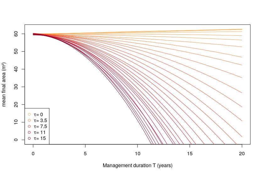
7Figure 3: Linear regression of mean final area as a function of management Figure 5: Quadratic regression curves of the mean final area as a function of T ,
duration T , with τ = 0.5 year−1 and initial population size = 1500. for different values of τ (low in clear colours, up to 15 mowings per year in dark
colours), and we set InitialPopS ize = 1500 and proportionMowing = 0.9.
project T , when τ > 2.5. Indeed, all the 50 regressions in the
sampling (variation of initial Population size and τ > 2.5) lead
to an R2 value larger than 0.95. The maximal value of RMSE
over these 50 regressions is 39 crowns, which is low compared
to the initial population size which has values 500 crowns or
1500 crowns.
Figure 6 gives an example of the quadratic regression on the
mean area for given values of τ and initial population size.
Figure 4: Quadratic regression of mean final area as a function of management
duration T , with τ = 8 year−1 and initial population size = 500. For the last
three points in the bottom right hand corner, at least half of the 50 simulations
lead to extinction.
These results give information about the influence of the du-
ration of the management project on stand growth. A first fact,
which is very important for management is that it is not suffi-
cient to mow to decrease the population size and area: if the
number of mowings per year is too low (less than 2.5 in our
case), the population size and area increase during the man-
Figure 6: Non linear regression of mean final size as a function of management
agement project. In Figure 5, we plot the quadratic regression duration project T with τ = 8 years−1 and initial population size = 500. For
curves for the average final area with respect to the duration of the last three points in the bottom right hand corner, at least half of the 50
the management project (T , on the abscissa), obtained for dif- simulations lead to extinction.
ferent τ. A second important fact for management is that we
cannot expect an eradication of a knotweed stand of initial area
60 m2 in less than 11 years (for 15 mowing events a year). The 3.2.2. Influence of the mean number of mowing events a year τ
figure also tells us about the stand surface reduction in terms In this section, we use the first sampling (sampling1) to study
of final mean area when mowing once more time per year. For the influence of the mean number of mowing events a year on
example, mowing 6 times a year instead of 5, during 10 years, the final mean areas and sizes. Given a value of initial popula-
reduces the final surface of the stand by 4 m2 on average (look- tion size and T , we perform
ing at the section T = 10 on Figure 5).
• a linear regression on strictly positive values of outputs for
As for the area, the size varies linearly for values of τ ≤ 2.5 the mean area.
(R2 around 0.9). For larger values of τ, we present here the
result of the non linear regression. • a non linear regression on strictly positive values for the
R2 and RMSE values enable us to conclude that the mean mean final population size, using the function f (τ) =
final size depends exponentially on the management duration InitialPopS ize ∗ exp(−τ/rate), with rate being a constant
8on which the algorithm nls minimizes the sum of squared Table 2: Summary of the regression results of Sections 3.2.1-3.2.3.
errors. This constant rate differs for each set of parameters
since it depends on the values of T and initialPopS ize. In Sections 3.2.1 to 3.2.3, we have studied the influence of
As mentioned for the similar constant in Section 3.2.1, we one parameter, while the two others were set constant. The
study this dependency in Section 3.2.4. two previous samplings introduced at the very beginning of this
Section 3.2 were designed to control the variation of manage-
The linear regression presented below holds for τ > 2.5 (as ment parameters and initial population size, in order to inves-
in Section 3.2.1) and T ≥ 2 (to have a decreasing population). tigate their influence on the model outputs. Based on results
R2 and RMSE values enable us to conclude that the mean fi- in Sections 3.2.1 to 3.2.3, we are now able to propose a for-
nal area depends linearly on the mean number of mowing events mula for the mean areas and sizes as a function of the two
τ. Indeed, 24 regressions over the 30 in the sampling (variation management parameters (the mean number of mowing events
of initial Population size and T ≥ 2) lead to an R2 value larger a year (τ) and the management project duration (T )) and the
than 0.95. The maximal value of RMSE over these 50 regres- initial population size. We use a Sobol sampling (that max-
sions is 2.09 m2 , which is low compared to the mean initial area imizes discrepancy of the sequence, i.e. the space is evenly
which has values 20 m2 or 60 m2 . covered) of 5000 points with τ ∈ [0; 15.0], T ∈ [0; 20], and
We also conclude that the mean final size depends exponen- initialPopS ize ∈ [100; 1500].
tially on the mean number of mowing events τ. Indeed, all the For the same reason as before, we consider the case of τ ≥ 2.5.
30 regressions in the sampling (variation of initial Population Equations (9) and (10) highlight relationships between final
size and T ≥ 2) lead to an R2 value larger than 0.95. The max- outputs, management parameters and initial population size.
imal value of RMSE over these 50 regressions is 64 crowns,
which is low compared to the initial population size which has Mean Final S ize = InitialPopS ize × exp(−T.(τ − a)/b), (9)
values 500 crowns or 1500 crowns.
with a, b ∈ R constants, and
3.2.3. Influence of the initial population size
Mean Final Area = max((c×τ+d)×T 2 +0.04×InitialPopS ize, 0)
In this section, we use the second sampling (sampling2) to
(10)
study the influence of the initial population size on the final
with c, d ∈ R constants.
mean areas and sizes. Given a value for τ and T , we perform
a linear regression on strictly positive values of outputs. Due We now discuss the results of the non linear regression with
to the wide range of values for the initial population size in the respect to the two management parameters (T and τ > 2) and
sampling2, too many extinctions may occur for a given set of initial population size (the sampling contains 4332 values for
management parameters. We thus perform the regression only the triplet (T , τ, InitialPopS ize)). R2 and RMSE between the
if there are at least 5 strictly positive output values. predicted values and the data for the mean size are respectively
R2 and RMSE values enable us to conclude that both the equal to 0.99 and 26.12 crowns. 95 % confidence intervals
mean final area and the mean final size depend linearly on ini- for the constants a and b are given by R and their values are:
tial population size. Indeed, in both cases, 60 regressions over a ∈ [0.90; 0.94] and b ∈ [20.46; 20.77]. R2 and RMSE be-
the 63 regressions among the 72 management sets in the sam- tween the predicted values and the data for the mean area are
pling lead to an R2 value larger than 0.95. The maximal value respectively equal to 0.99 and 2.23 m2 . Moreover, the corre-
of RMSE over these 63 regressions is 1.1 m2 (resp. 18 crowns) sponding 95 % confidence intervals for the constants c and d
for the mean final area (resp. the mean final size) case, which is are c ∈ [−0.0342; −0.0336] and d ∈ [0.0960; 0.0998], respec-
low compared to the mean initial area (resp. initial population tively. Taking T = 0 in the right hand side of Equations (9) and
size) which ranges from 2 m2 to 48 m2 (resp. from 50 crowns (10), gives InitialPopS ize and InitialPopS ize ∗ 0.04, respec-
to 1200 crowns). tively. The last quantity thus corresponds to the mean initial
Notice that the influence of the initial population size on the area. There is indeed a linear dependency between the mean
initial area is also linear. Indeed, the sampling2 contains the initial area and the initial population size.
case T = 0, and for this specific value of T the final area is the An important remark on the generality of Equations (9) and (10)
initial area. is the following: results obtained for the mean output quantities
are still relevant for direct outputs, without considering mean
3.2.4. Formulas for the mean final sizes and areas, as functions
quantities. Figure 7 illustrates this point, plotting the formula
of τ, T and the initial population size
(9), for given values of τ and initial population size and by let-
We summarize results of the regressions we performed in Ta- ting T vary. We emphasize that the red line on Figure 7 has
ble 2. been found with a regression on a far larger set of points than
Parameter mean output Variation R2 > 0.95 RMSE the subset selected to plot this example.
T for τ ≥ 2.5 final area quadratic & 47/50 1.31 Equations (9) and (10) enable us to find which parameter most
T for τ ≥ 2.5 final size exponential & 50/50 39 influences model outputs, and thus on which one it is better to
τ for τ ≥ 2.5 final area linear & 24/30 2.09
τ for τ ≥ 2.5 final size exponential & 30/30 64 concentrate management efforts. To do so, we compared for
InitialPopS ize final area linear % 60/63 1.1 each value of the triplet (T ,τ,InitialPopS ize) the final size and
InitialPopS ize final size linear % 60/63 18 area according to Equations (9) and (10), for the three following
9Figure 7: Exponential regression for the mean final size as a function of the Figure 8: Parameters having the greatest influence on final size. Each plot
management duration project (T ). The red line is the prediction function of corresponds to a fixed value of InitialPopS ize specified above the plots (from
T defined by Equation (9). Black circles represent stand sizes resulting of 50 100 to 1500 crowns), τ varies on the x-axis, and T varies on the y-axis.
replications with τ = 4, initial population size = 1000, letting T vary.
parameter value combinations: (T + 1,τ,InitialPopS ize), (T ,τ +
1,InitialPopS ize) and (T ,τ,InitialPopS ize × 0.9). Each plot on
Figures 8 and 9 corresponds to a fixed value of InitialPopS ize,
with τ varying on the x-axis and T varying on the y-axis, and
associates with each triplet the most important parameter in a
management perspective, that is the parameter the modification
of which produces the lowest output (it happens that two mod-
ifications produce the lowest output). Brown zones correspond
to set of parameter values that lead to eradication, thus in this
zone no gain can be expected by any modification. Figure 8
shows that, out of the extinction zones, T or τ have the greatest
influence on final size and allows to determine the most efficient
management modification. Especially, when τ is low, it is more Figure 9: Parameters having the greatest influence on final area. Each plot
efficient in terms of size reduction to mow one more time each corresponds to a fixed value of InitialPopS ize specified above the plots (from
100 to 1500 crowns), τ varies on the x-axis, and T varies on the y-axis.
year, and conversely, when T is low, it is more efficient to con-
tinue mowing one more year. As for the final area, we observe
on Figure 9 that areas corresponding to a greatest influence of
T or τ are reduced compared to Figure 8, in the favor of the area ters (for τ > 2.5) and initial population size. We have shown
of greatest influence of InitialPopS ize. In these regions of pa- that mowing is not sufficient to decrease the population size
rameter values, beginning the management project on smaller and area. Indeed, if the number of mowing events per year is
stands (size equal to 90% of reference size) has more impact on too small (smaller than 2.5 in our case), the population size and
the final area than mowing one more time each year or over a area increase during the management project. We have also
one year longer period of time; thus in these conditions, early shown how those results could be used by managers. Simu-
detection of stands should be encouraged. lation results suggest the minimal duration of the management
project necessary to achieve eradication (if it is possible at all,
given a certain frequency of mowing). In Figure 5, we plotted
4. Discussion the quadratic regression curves for the average final area with
respect to the duration of the management project (T ), obtained
In this paper, we proposed a stochastic individual based model for different values of τ and for given values of InitialPopS ize
for the growth of a stand of Japanese knotweed including mow- and proportionMowing. The figure indicates the potential ben-
ing as a management technique. Then, we calibrated plant dy- efit in terms of invaded area reduction, of mowing the stand
namics parameters with field data in Section 3.1. The set of once more each year. More generally, formulas given in Equa-
parameters obtained was in agreement with values of param- tions (9) and (10), highlighting the relation between final out-
eters available in the literature and with our field experience. puts, management parameters and initial population size, en-
In Sections 3.2.1 - 3.2.3 we studied the influence of the initial able to answer questions about the efficiency of different mow-
population size, the mean number of mowing events a year and ing strategies.
the management project duration on mean area and mean size Following Dauer and Jongejans (2013) and Smith et al. (2007),
of stands. We also obtained formulas for the area and size of we have assumed that the invasion occurs in an homogeneous
a knotweed stand, as functions of those management parame- area. Models that take into account the inhomogeneities of the
10invaded land are often static models, which do not consider the funding from the Chair "Modélisation Mathématique et Biodi-
invasion as a dynamic phenomenon (no temporal component versité" of VEOLIA-Ecole Polytechnique-MNHN-F.X. FL and
(Lookingbill et al., 2014; Buchadas et al., 2017)). Lookingbill BR also acknowledge partial funding through the ANR "Alien"
et al. (2014) use indices such as habitat suitability, constructed project (ANR 14-CE36-0001-01). Finally, IA, FL, SM and CS
from field data such as humidity or soil type, to produce inva- acknowledge Complex System Institute of Paris Île de France
sibility maps. These maps assign a score to each zone which for the hosting, and the OpenMOLE team for their advice on
describes its probability of being invaded. the software.
Another simplification in our model is that we did not take into
account the dispersal of fragments of rhizome due to mowing.
Appendix A. Summary of model parameters
This may however be an important way of propagation of the
plant in some conditions and it contributes to its invasiveness Table A.1 focuses on the plant dynamic parameters. We precise
(Sásik and Eliás, 2006). Dispersal has to be considered if one parameters units for those that have a biological meaning.
wants to model the invasion of Japanese knotweed at the scale
of a region composed of several stands. This will be the subject Variable Description unit
Biomass
of future work. We could formulate this problem in the formal- K maximal biomass (Equation (5)) g
ism of the viability theory (Aubin, 1991). In this framework, L biomass growth rate for low biomass (Equation (5)) year−1
a0 initial biomass (of a crown at birth) g
the dynamics of the system depends on the system state and on Mowing
controls. One objective is to prove the existence of controls and mowingParameter in the mowing effect function in Equation (3) g−1
to find initial values of the system such that the system state Mortality
deathParameterS caling mortality rate for the low biomasses in Equation (7) year−1
remains in a set of constraints (e.g. the invaded area below a deathParameterDecrease decay rate of mortality function in Equation (7) g−1
given threshold). For example, managers could be interested in Birth
distanceParent apical dominance distance (Equation (1)) m
controlling the density of Japanese knotweed. Then we could distanceCompetition intraspecific competition distance (Equation (2)) g
b̄ birth rate (under ideal conditions) year−1
study the resilience of the system, that is to say its ability to (shape, scale) Gamma law, dispersion of the new individual
recover a property after a perturbation.
The importance of integration (biomass transfer between Table A.1: Summary of model parameters
crowns) is still under debate. In Price et al. (2002), the authors
notice that there is relatively few integration, whereas in Suzuki We have the following management parameters:
(1994) the authors found a larger integration. We did not con-
sider this process in our model. Adding this phenomenon could • mean number of mowing events a year: τ
produce simulation results closer to reality. • management project duration: T
The field data we have used for the calibration were extracted
from Martin et al. (2018). The measurements were carried out • proportion of mown crowns: proportionMowing
in 2008 and 2015 on stands that were mown or not. For each
stand, data provide some information about the management and initial population size parameter: InitialPopS ize.
technique used by the land owner: the frequency of mowing
and an estimation of the proportion of the mown stand. Calibra- Appendix B. Description of the algorithm used to simulate
tion results for some of the plant dynamics parameters based on a solution of Equation (8).
these measurements are in agreements with data found in the
literature. We present one step of the algorithm that enables to make
The model is written in the formalism of measure-valued evolve a stand under mowing.
stochastic processes. The tools we used here for the particu- At each time, there are three possible events: a birth, a death or
lar case of the management of a Japanese knotweed stand can the mowing of a proportion proportionMowing of individuals
be used in a more general context. In particular, we could ap- in the population. Suppose we have N individuals at a time t.
ply this method to others invasive plants, like seed dispersal We start by calculating the next time at which there is an event,
species. One could even allow individuals to move in such which requires the sum of the rates of the events of birth, death
models. In Leman (2016), the author took into account the spa- and mowing). The law of this time only depends on the current
tial motion in an individual-based stochastic population model. population state as the process is Markovian.
Furthermore, including sexual reproduction of individuals, as If it is a birth event, we select the parent uniformly at random
in Smadi et al. (2018), would also enable to consider animal in the population. We check whether the individual selected to
invasive species, like mosquitoes (Juliano and Philip Lounibos, be the parent does not already have too many neighbours at a
2005) or feral cats (Baker and Bode, 2016). distance lower than distanceParent. If it occurs, we draw the
position of the new individual (child) according to the Gamma
Aknowledgements law described in the paragraph "Dispersal of the created indi-
vidual" of Section 2.1 (with an angle chosen uniformly around
This work was partially funded by Electricité De France (EDF) the potential parent). If the child’s position falls into the set C
and we thank Laure Santoni and Agnes Bariller for helpful dis- of Equation (2) (i.e. it does not fall into an intraspecific com-
cussions and comments. FL, SM and CS acknowledge partial petition zone), then the individual is born at this position, and
11You can also read