MI OFFSET 2018 User's Guide: Fundamental Principles, Development History, and User Manual - Enviroweather
←
→
Page content transcription
If your browser does not render page correctly, please read the page content below
MI OFFSET 2018 User’s Guide: Fundamental
Principles, Development History, and User Manual

                             M ICHAEL T. K IEFER
                           A SSISTANT P ROFESSOR
      D EPARTMENT OF G EOGRAPHY, E NVIRONMENT, AND S PATIAL S CIENCES
                        M ICHIGAN S TATE U NIVERSITY
                     673 AUDITORIUM ROAD , ROOM 204
                      E AST L ANSING , M ICHIGAN , 48824
                             mtkiefer@msu.edu

                        Last updated: January 17, 2018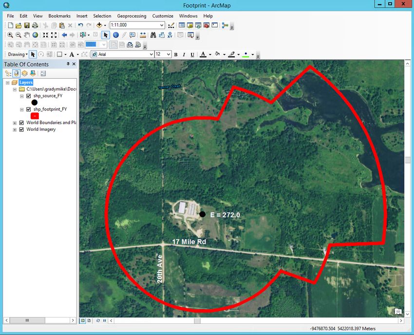
Contents
1   Introduction                                                                          3

2   MN OFFSET                                                                              3
    2.1 Background                                                                         3
    2.2 Livestock odor field measurements                                                  3
          Supplemental: Odor Testing Primer                                                4
          Supplemental: Additional Field Studies                                           6
    2.3   Dispersion model evaluation                                                      7
          2.3.1 INPUFF-2 introduction                                                      7
          Supplemental: Gaussian dispersion models                                         7
          2.3.2 Short distance evaluation: Up to 500 m from source                         8
          2.3.3 Long-distance evaluation: Up to 3.2 km from source                         8
    2.4   Empirical setback distance - odor emission rate relationship                     8
          2.4.1 Characterizing atmospheric dispersion potential                            8
          2.4.2 INPUFF-2 Simulations                                                       9
          Supplemental: Odor emission terminology                                         10
          2.4.3    State-wide atmospheric dispersion climatology                          11
          2.4.4    State-wide odor annoyance climatology                                  12
          2.4.5    Adaptation for local climatology                                       13

3   MI OFFSET 2000                                                                        13
    3.1 Background                                                                        13
    3.2 Differences between MI OFFSET 2000 and MN OFFSET                                  14
    3.3 Construction of odor footprint                                                    15
          Supplemental: MI OFFSET 2000 Odor-Annoyance Frequency Methodology               16
    3.4   Known limitations of MI OFFSET 2000                                             17

4   MI OFFSET 2018                                                                        17
    4.1 Background                                                                        17
    4.2 Updated wind and atmospheric stability climatology                                18
        4.2.1 Introduction to NARR                                                        18
        4.2.2 NARR wind assessment and wind speed adjustment                              19
        4.2.3 Selection of method for estimating Pasquill class                           21
        4.2.4 NARR-based Pasquill class: Methodology                                      21
        4.2.5 NARR-based Pasquill class: Evaluation                                       22
          Supplemental: Evaluation of Methods for Selection of 1.5%, 3%, and 5% Classes   24
    4.3   Construction of odor footprint                                                  26
    4.4   On-demand odor footprint tool                                                   26
          4.4.1 Transition from Microsoft Excel spreadsheet to web tool                   26
          4.4.2 Web tool interface                                                        27
          4.4.3 Web tool output                                                           32

                                                   1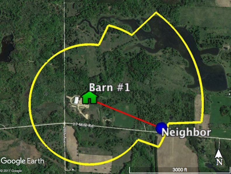
4.4.4   Export to GIS applications: Google Earth and ArcGIS   36

5   Bibliography                                                      43

                                            2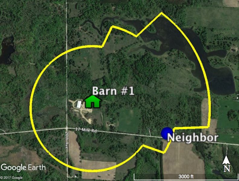
1. Introduction
   As the title of this document suggests, it has been prepared with three goals in mind:

    • (1) Describe the basic principles underpinning the Odor from Feedlots – Setback Estimation
      Tool (OFFSET) model [Fundamental Principles].

    • (2) Trace the evolution from the original OFFSET developed for use in Minnesota, here-
      after MN OFFSET, to MI OFFSET 2000, the first version of OFFSET developed for use in
      Michigan, and finally, to the revised MI OFFSET 2018 [Development History].

    • (3) Provide instructions that explain to any user familiar with MI OFFSET 2000 how to run
      MI OFFSET 2018 [User Manual].

  This document is organized in chronological order: MN OFFSET is discussed in section 2, MI
OFFSET 2000 is discussed in section 3, and MI OFFSET 2018 is discussed in section 4.

   Gray boxes are used in this document to denote supplemental information that, while not
   essential to an understanding of MI OFFSET 2018, may be of interest to some readers.

2. MN OFFSET
2.1. Background
    In 1997, the Livestock Odor Task Force (LOTF) of Minnesota recommended development of a
tool for prediction of offsite odor movement from livestock operations. The MN OFFSET model
was developed based on this recommendation. For complete documentation of MN OFFSET, see
Jacobson et al. (2005) and Guo et al. (2005).

2.2. Livestock odor field measurements
    Odor measurements from four separate field campaigns were used in the development of MN
OFFSET.
    The first field study was performed to establish reference odor emission rates for various types
of livestock housing and manure storage facilities (Jacobson et al. 2000). Air samples and venti-
lation rate measurements were collected in animal production buildings and manure storage units
at 85 farms in Minnesota. Within 24 hours of air sample collection, the odor detection threshold
of each air sample was determined in a laboratory using an instrument known as an olfactometer
(McGinley et al. 2000; Jacobson et al. 2005).
    The terms “odor detection threshold”, “odor concentration”, and “odor dilution threshold” are
used interchangeably in the literature (e.g., McGinley et al. 2000; Zhu et al. 2000; Jacobson et al.
2005; Guo et al. 2005). In this document, the term “odor detection threshold” is used, as it is the
term that is used most often in the MN OFFSET documentation (Jacobson et al. 2005; Guo et al.
2005). In reviewing the history of MN OFFSET, it is helpful to keep in mind that the higher the

                                                 3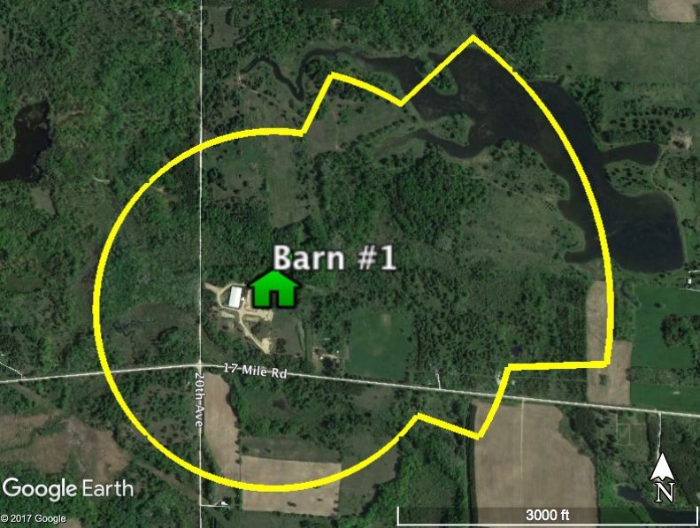
odor detection threshold, the greater the odor concentration of the original air sample.

                                Supplemental: Odor Testing Primer

   The following information is drawn primarily from McGinley et al. (2000) [“Odor basics:
   Understanding and using odor testing”].

   It is critical to note that measuring odor concentration directly is made impractical by
   the weak relationship between the detectability of an odor and the mass concentration
   of the odorous molecules causing it. Thus, odor concentration is measured indirectly by
   progressively mixing greater and greater quantities of clean air with the original air sample
   until the odor is undetectable by half of the members of a panel of human observers. The
   number of dilutions required to render the odor effectively undetectable is used as a measure
   of the odor concentration of the original air sample. An important term to understand is the
   “dilution ratio”, which is the ratio of the volume of the diluted air sample to the volume of
   the original air sample. For example, if the volume of the original air sample is 10 cm3 , and
   the sample has to be mixed with 1000 cm3 of clean air before the odor is undetectable to
   half of the members of an odor panel, then the dilution ratio is 1010 / 10 = 101.

   A panel of six to ten trained assessors are presented with diluted air samples, and using a
   method known as “ascending concentration series”, progressively less diluted air samples
   are provided to each panelist until they are able to detect, but not necessarily identify, an
   odor (comparing the diluted air sample to two samples of clean air). For each panelist, their
   individual “estimated detection threshold” is determined by geometrically averaging the
   dilution ratio of the air sample in which they first detected the odor, and the dilution ratio of
   the preceding (more diluted) air sample. For example, if the odor was first detectable at a
   dilution ratio of 500, then their
                                h√ estimated detectioni threshold is 707, which is the geometric
   average of 500 and 1000         500 ∗ 1000 = 707 . Finally, the “odor detection threshold”
   for the original sample is determined by computing the geometric mean of the individual
   estimated detection thresholds for the entire panel, and is interpreted as the number of
   dilutions needed to make the odor sample undetectable by 50% of the human population.

   Although the dilution ratio itself is dimensionless, the odor detection threshold is given
   “pseudo-dimensions” of odor units [OU] or odor units per cubic meter [OU m−3 ], the latter
   units being analogous to mass concentration units of kg m−3 .

    Subsequently, emission rates for each source category (e.g., dairy, free stall housing) were
computed as the product of odor detection threshold and ventilation rate, normalized by the area of
the source, and were geometrically averaged over all data samples from that category. The result
of this process was a pair of lookup tables giving odor emission references rates for various animal
housing and manure storage types. In addition, various odor control technologies were researched
and a lookup table of odor control factors was developed (Fig. 1).

                                                  4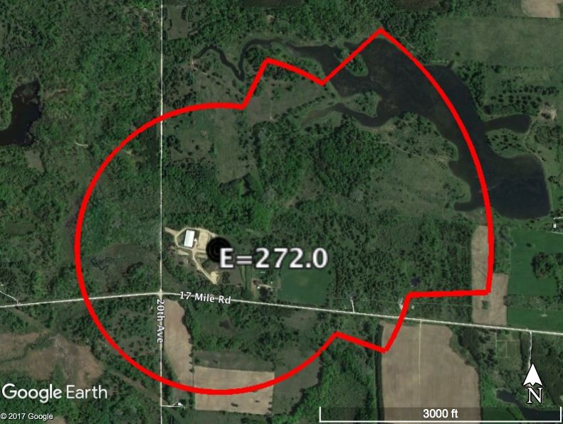
Figure 1: Odor emission reference rates for animal housing (a) and manure storage (b), and odor con-
trol factors for selected technologies (c), as developed for MN OFFSET (reproduced from Jacobson et al.
(2005)). Numbers outside parentheses are observed values, numbers inside parentheses represent scaled
odor emission rates (see section 2.3.1). Note that the scaled odor emission rates, and odor control factors,
are similar and in some instances identical to those used in MI OFFSET 2000 and MI OFFSET 2018.

                                                     5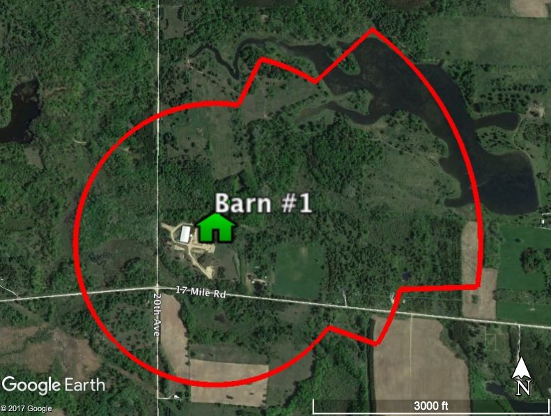
Supplemental: Additional Field Studies

The second field study was performed in order to develop a relationship between odor
detection threshold, determined using olfactometers in the laboratory, and odor intensity,
measured by trained nasal field assessors using number and word categories to describe
the odor (Guo et al. 2001). Air samples taken in the odor plume downwind of the source
are generally below the sensitivity threshold of olfactometers, requiring the use of field
observers and a subjective odor intensity scale. Observers judged odor intensity by
comparing air samples from the odor plume to a reference n-butanol scale; intensity was
assigned by choosing the n-butanol intensity level of the same or similar strength to the
odor sample. The relationship between odor detection threshold and odor intensity was
developed based on 124 paired odor intensity and odor detection threshold measurements
(from 60 swine buildings, 66 swine manure storage facilities, and 55 dairy and beef farms,
in MN). The relationship between the two metrics is represented as an exponential function
Z = aeb∗I , where Z is odor detection threshold [OU m−3 ], I is odor intensity (on a 0-5
scale), and a and b are coefficients specific to swine and cattle odor sources. Note that each
odor intensity level covers a range of odor detection thresholds, for example odor intensity
level 1 for swine odor corresponds to 5-42 OU m−3 , and odor intensity level 3 for cattle
odor corresponds to 142-420 OU m−3 .

The third study was conducted in order to produce a dataset with which to validate the
dispersion model used in the development of OFFSET, INPUFF-2, over distances up to
500 m from the odor source. Short-distance odor plume measurements were made using
trained nasal field assessors positioned downwind of odor sources at 28 Minnesota farms
(Jacobson et al. 1998). Data collected during this study consisted of odor samples used to
estimate odor emission rates, odor intensity measurements taken by nasal field assessors in
the odor plume downwind of the odor sources, and on-site weather information, including
wind speed and direction, solar radiation, temperature, and relative humidity, required by
the INPUFF-2 model. A total of 368 short-distance odor intensity measurements were made
using a 0-5 odor intensity scale.

The fourth and final study was performed in order to obtain long-distance odor measure-
ments, up to 3.2 kilometers downwind of the source, for the validation of long-distance
smoke predictions in INPUFF-2. A different approach than that used for short-distance mea-
surements was required because it is difficult to predict the location and timing of the odor
plume at such distances, making the positioning of field assessors difficult if not impossible.
Thus, a total of 296 long-distance odor measurements were made using a simpler 0-3 odor
intensity scale, inside a 4.8 km x 4.8 km grid of farmland by trained local resident odor ob-
servers (Guo et al. 2001). Like the previous study, data collected during this study consisted
of odor samples, odor intensity measurements, and on-site weather information required by
the INPUFF-2 model.

                                              6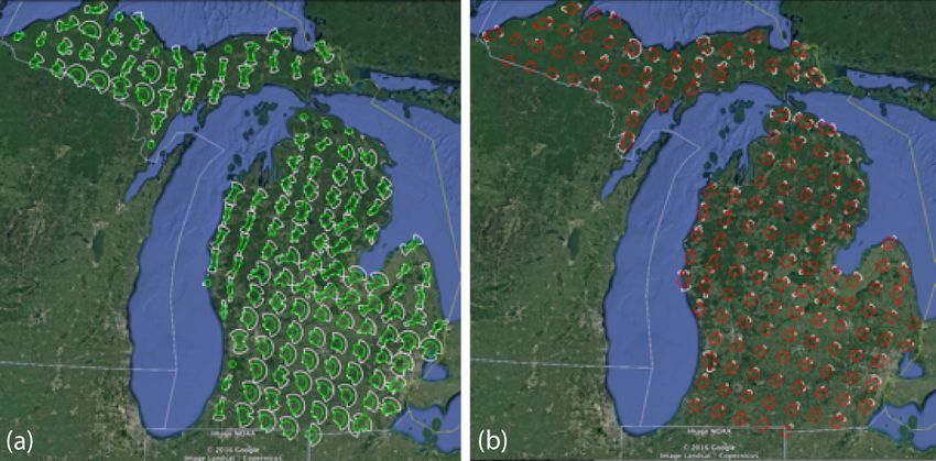
2.3. Dispersion model evaluation
   2.3.1) INPUFF-2 INTRODUCTION
    INPUFF-2 is a Gaussian puff model developed by the U.S. Environmental Protection agency
for use in predicting mass concentration over short time periods downwind of one or more sources
(Petersen and Lavdas 1986). INPUFF-2 was utilized in the development of MN OFFSET in order
to explore the relationship between odor emission rate, atmospheric conditions (wind speed and
stability), and odor detection threshold (i.e., concentration) at various distances from the source.
The impracticality of examining this relationship from observations alone, due to the multiple de-
grees of freedom involved, necessitated the use of a dispersion model.

                            Supplemental: Gaussian dispersion models

   As transport and dispersion models vary widely in complexity, and a full review of models is
   beyond the scope of this document, this brief summary focuses on Gaussian plume and puff
   models. For a review of dispersion models in the context of odor transport and dispersion,
   see Guo et al. (2006). Gaussian plume models predict the dispersion of a point source of
   pollutants, whether elevated or ground level, assuming a steady-state source and steady-
   state atmospheric conditions. “Gaussian” refers to the assumption of a Gaussian probability
   distribution of the pollutant downwind of the source, an assumption that implicitly accounts
   for turbulent diffusion of pollutants in three-dimensions. The concentration of pollutants is
   greatest at the center of the plume, and decays exponentially with distance from the plume
   center. One can imagine the plume in a Gaussian plume model as a cone aligned with the
   mean wind, anchored at the source, that grows in diameter with downwind distance from the
   source. Gaussian puff models, like INPUFF-2, are similar to Gaussian plume models, except
   that (i) the pollutant source is not assumed steady-state, and (ii) the atmospheric conditions
   are allowed to vary in time and space. The pollutant is released in discrete “puffs”, that
   expand in size with distance downstream of the source. The distribution of the pollutant
   across the puff is assumed Gaussian, as in the Gaussian plume model. The plume in a
   Gaussian puff model can be visualized as a cone, like the Gaussian plume model, but with
   the pollutants contained within puffs or clouds that grow in size as they move away from the
   source.

    A preliminary assessment of INPUFF-2 odor plume predictions revealed the need to apply
“scaling factors” to the observed odor emission rates (Fig. 1) before ingesting them into INPUFF-
2, in order to obtain odor detection threshold output from INPUFF-2 that, to quote Zhu et al. (2000),
“fell into the same numerical range as the field data”. Zhu et al. (2000) argued the the use of scaling
factors was justified because INPUFF-2 is a Gaussian model developed for use in predicting mass
concentrations (such as for particulate matter), and the mass of odor molecules is unknown. Thus,
scaling factors allow Gaussian models, developed specifically for mass dispersion applications, to
be applied to the problem of odor dispersion, provided the scaling factors are verified by extensive
field tests.

                                                  7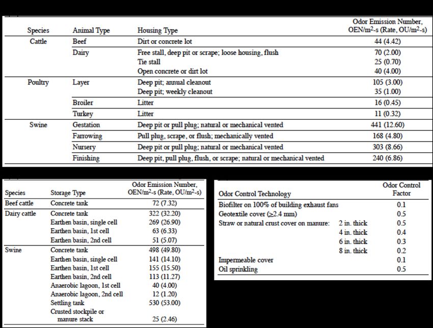
2.3.2) S HORT DISTANCE EVALUATION : U P TO 500 M FROM SOURCE
    At points spanning the odor plume, odor detection threshold observed by field assessors [con-
verted from odor intensity via an empirical relationship discussed earlier in section 2.2, Supple-
mental: Additional Field Studies], were compared to odor detection threshold values output by
INPUFF-2; this process was repeated at distances of 100, 200, 300, 400, and 500 m from the odor
source. A total of approximately 30 single and multiple source events were simulated, and as the
odor measurements were made on different days at different times of day, a variety of atmospheric
conditions were considered. The Wilcoxon Signed Rank Test was used to compare field measure-
ments and INPUFF-2 predictions, revealing 80-95% confidence in using INPUFF-2 at distances of
100-300 m from the odor source, with poor model performance noted at distances of 400-500 m
from the source (possibly attributable to human measurement errors at low odor levels).

   2.3.3) L ONG - DISTANCE EVALUATION : U P TO 3.2 KM FROM SOURCE
    A total of 170 long-distance odor dispersion events were simulated by INPUFF-2, most of
which occurred during the early morning, evening, and night. All odor events occurred within
a 4.8 km x 4.8 km odor monitoring grid in rural Minnesota inside which trained resident odor
observers reported odor intensity on a 0-3 scale, along with time of measurement, and relevant
weather conditions (temperature, relative humidity, wind speed and direction, and solar radiation).
Only odor events for which the odor source was located inside the 4.8 km x 4.8 km monitoring
grid were considered in the model validation exercise. An INPUFF-2 prediction was considered
correct if the predicted odor detection threshold fell within the range of odor detection thresholds
corresponding to the odor intensity measurement [see section 2.2, Supplemental: Additional Field
Studies]. Given the broad range in odor detection thresholds corresponding to each odor intensity
level, the evaluation methodology is arguably generous. For example, if the measured odor in-
tensity downwind of a swine farm was 2 [124-1070 OU m−3 ], and INPUFF-2 predicted an odor
detection threshold anywhere within the range of 124-1070 OU m−3 , the INPUFF-2 prediction was
deemed satisfactory. A general conclusion of the long distance evaluation study was that INPUFF-
2 performed most satisfactorily for low-intensity odor events, but tended to underestimate odor
detection threshold for higher-intensity odors. The limited number of moderate- to high-intensity
odor events renders this result low-confidence.

2.4. Empirical setback distance - odor emission rate relationship
   2.4.1) C HARACTERIZING ATMOSPHERIC DISPERSION POTENTIAL
    Six wind-stability classes were defined during the development of MN OFFSET, based on wind
speed and Pasquill stability class (Pasquill 1961), in order of increasing potential for atmospheric
dispersion or mixing (Table 1; WC1: least dispersed, WC6: most dispersed).

                                                 8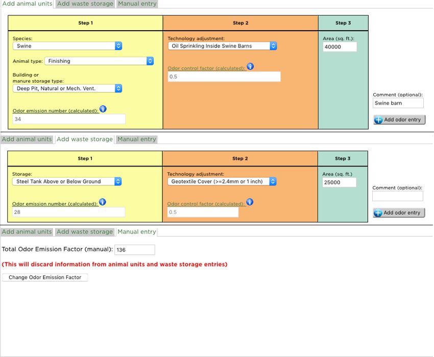
Table 1: Definition of MN OFFSET wind-stability classes.
              Name     Pasquill Class                  Wind speed (S) range
              WC1            F                       S ≤ 1.3 m s−1 (2.9 mph)
              WC2            F           1.3 m s (2.9 mph) < S ≤ 3.1 m s−1 (6.9 mph)
                                                −1

              WC3           E                        S ≤ 3.1 m s−1 (6.9 mph)
              WC4           E            3.1 m s−1 (6.9 mph) < S ≤ 5.4 m s−1 (12.1 mph)
              WC5           D                       S ≤ 5.4 m s−1 (12.1 mph)
              WC6           D           5.4 m s−1 (12.1 mph) < S ≤ 8.0 m s−1 (17.9 mph)

     The Pasquill classification scheme has been widely used in dispersion applications (e.g., smoke,
power plant emissions, odors) to describe the ability of the atmosphere to dilute pollutants. Dif-
ferent forms have been developed since the original 1961 study, but the most common form uses
six classes, ordered from greatest mixing/dispersion potential to weakest mixing/dispersion poten-
tial: A (strongly unstable); B (moderately unstable); C (weakly unstable); D (neutral); E (weakly
stable); F (strongly stable). This is the form used by MN OFFSET. Note that under unstable con-
ditions (classes A-C), odors are strongly mixed with ambient air and odors become well-diluted
over short distances from the source; thus, classes A-C were neglected in MN OFFSET and all
subsequent OFFSET tools.

   2.4.2) INPUFF-2 S IMULATIONS
    Setback distance (D) is defined in Guo et al. (2005) as the distance downwind of a livestock
production site where the odor detection threshold is reduced to 75 OU m−3 , i.e., where the odor
intensity is a 2 (faint odor) on a 0-to-5 n-butanol intensity scale [conversion from field-measured
intensity to odor detection threshold follows from the second field experiment described in section
2.2, Supplemental: Additional Field Studies]. Beyond the setback distance, odor is considered to
be mostly undetectable by the general population. Interestingly, when validating INPUFF-2 (Zhu
et al. 2000; Guo et al. 2001), a particular odor intensity level translated to a range of odor detection
thresholds (e.g., odor intensity level 2 = 42-124 OU m−3 ), but in defining the setback distance, a
single odor intensity level was assumed equivalent to a single value of odor detection threshold
(e.g., odor intensity level 2 = 75 OU m−3 ).
    A relationship between D and total odor emission factor (E) under different atmospheric con-
ditions was the primary goal of the developers of MN OFFSET. Note that E is computed as the
product of odor emission reference rate (units: OU m−2 s−1 ), odor source area (units: m2 ), and
odor control factor (units: none), and has units of OU s−1 . Odor emission reference rates and odor
control factors are obtained from the look-up tables in Fig. 1.

                                                   9
Supplemental: Odor emission terminology
A few technical points about odor terminology, dimensions, and units in the MN OFFSET
documentation are worth mentioning here: (1) odor detection threshold, used to compute the
odor emission reference rate, was given what McGinley et al. (2000) refer to as “pseudo-
dimensions” as part of the odor testing described in section 2.2, Supplemental: Odor Testing
Primer. Although these dimensions are not physical in nature, they are the given dimensions
of odor detection threshold, and the dimensions of any quantities derived from odor detection
threshold are based on them; (2) The odor emission reference rate is not really a rate, but a
flux [it has flux dimensions, i.e., change in quantity per unit of time per unit of area]; (3) E
is referred to as a dimensionless quantity in Guo et al. (2005), but it is actually a rate, with
units of OU s−1 [these are rate dimensions, i.e., change in quantity per unit of time].
For consistency with OFFSET literature and real-world application, E will hereafter be pre-
sented without units and scaled by 104 (e.g., E=108, E=342).
Following the field experiments, an undefined number of simulations with the INPUFF-2 dis-
persion model were performed in which wind-stability conditions and odor emission rates (i.e., in-
puts) were varied independently, and odor detection threshold at various distances from the source
was output by the model. Analysis of the dispersion model simulations yielded an empirical rela-
tionship between odor detection threshold at a given distance downwind of a source, odor emission
rate, and wind-stability class. The odor annoyance threshold of 75 OU m−3 [odor intensity rating
of 2 on a 0-5 scale] allowed for a determination of D from the INPUFF-2 output, and a power law
relationship between D and E was subsequently developed:
D = aE b (1)
where a and b are “weather influence factors” that account for the ability of the atmosphere to
mix and disperse odors. The a and b coefficients, along with resulting values of D (in meters) for
a hypothetical farm with E=108 are provided in Table 2.
Table 2: MN OFFSET weather influence factors a and b, along with setback distances (D) for E=108.
Name a b D [m]
WC1 1.685 0.513 2016.5
WC2 0.729 0.537 1215.4
WC3 0.446 0.540 775.1
WC4 0.180 0.584 574.5
WC5 0.131 0.583 412.4
WC6 0.051 0.626 290.8
Interpretation: in order to only barely detect the odor (and thus not generally be bothered by
it) under the most stable, lightest wind conditions, an observer would need to be about ten times
farther from the source than under the least stable, windiest conditions. The relationship may be
visualized for a range of E as shown in Fig. 2 [reproduced from Fig. 1 in Guo et al. (2005)],
10wherein each line corresponds to a different wind-stability class. The annoyance-free labels in Fig.
2 are described in section 2.4.4.
Figure 2: Setback distances for different weather conditions from animal production sites. The odor-
annoyance-free frequencies are the averages for Minnesota. Weather conditions given are atmospheric
stability class and wind speed. Reproduced from Guo et al. (2005).
2.4.3) S TATE - WIDE ATMOSPHERIC DISPERSION CLIMATOLOGY
The purpose of this analysis was to determine how frequently the six wind-stability classes
occur in general across Minnesota, and then assign odor-annoyance-free frequencies to each line
in the setback distance chart (Fig. 2). This allows a user to estimate the minimum separation
distance between source and neighbor that is necessary for the neighbor to be odor-annoyance-free
some percentage of the year (e.g., 97% annoyance free), for a given total odor emission factor (e.g.,
E=108).
Hourly weather data from six weather stations in the upper Midwest (Duluth, MN; International
Falls, MN; Minneapolis-St. Paul, MN; Rochester, MN; Sioux Falls, SD; Fargo, ND) over a 9-year
period were used to construct a quasi-climatology of wind and atmospheric stability aimed at
determining the annual frequency of the six wind-stability classes defined in section 2.4.1. Note
that the hourly weather data used in the development of MN OFFSET, as well as MI OFFSET 2000,
were obtained from the EPA Support Center for Regulatory Air Models (EPA-SCRAM) program.
Note that the EPA-SCRAM dataset is limited to 1984 –1992. Pasquill class was determined using
a method that takes as input 10-m wind speed, solar insolation (daytime), and cloud cover in octas
(nighttime).
For each weather station, a graphic known as a windstar chart was computed depicting the
cumulative frequency of the six wind-stability classes for each 22.5 degree-wide wind direction bin
(Figure 3; directions indicate the direction the wind is blowing from). The cumulative frequency is
11the frequency of a particular wind-stability class -or- more stable conditions. The rationale behind
the use of cumulative frequency is that it represents a sort of worst-case-scenario frequency. For
example, examining Fig. 3, we see that there is a 1.9% probability of WC4 (E≤5.4) or more stable
conditions -and- a wind from the north [between 348.75 and 11.25 degrees; see blue circle in
figure]. Thus, conditions less stable and more windy than WC4, or winds blowing from a different
direction, are expected to occur at least 98.1% of the time. If a setback distance is computed
assuming WC4 conditions and a north wind, a neighbor to the south might detect odors up to 1.9%
of the time, that is, they are expected to be odor-annoyance-free at least 98.1% of the time.
Figure 3: Annual windstar chart for Minneapolis-St. Paul, Minnesota, from 1984 –1992 [Jacobson et al.
(2000), reproduced in Jacobson et al. (2005)].
2.4.4) S TATE - WIDE ODOR ANNOYANCE CLIMATOLOGY
Each wind-stability class was examined individually, and the highest frequency of any direction
was chosen as the worst-case scenario frequency. For any other wind direction, the frequency of
occurrence would be lower. For example, for F≤3.1 (WC2; green lines and symbols), the highest
frequency on the Minneapolis-St. Paul windstar chart is 1.7% (SW wind prevails). For any other
wind direction, the frequency of that wind-stability condition (or more stable conditions) is less
than 1.7%. This worst-case-scenario frequency was determined for each station and then averaged
among the six stations. This was repeated for each wind-stability class. This yielded, for each
wind-stability class, a single worst-case-scenario occurrence frequency to be applied state-wide.
12The state-wide frequencies first presented in Jacobson et al. (2000), and reprinted in Jacobson et al.
(2005) are as follows:
WC1: 1%; WC2: 2%; WC3: 3%; WC4: 4%; WC5: 6%; WC6: 9%
The inverse of this frequency is the frequency of conditions less stable, and thus less conducive
to bothersome odors, than the particular wind-stability class. For example, under the worst-case-
scenario, conditions less stable and therefore more dispersive (i.e., dilutive) than WC2 are expected
to occur 98% of the time. In all likelihood, the frequency of these less-bothersome odor conditions
would exceed 98%.
The calculation of the state-wide wind-stability class frequencies allowed the developers of MN
OFFSET to label the setback distance lines in Figure 2, each corresponding to a particular wind-
stability class, as the frequency of odor-annoyance-free conditions (for example, the WC2 line is
labeled 98% odor-annoyance-free. This allows the user to estimate how much distance between
their farm and their downwind neighbor is necessary for the neighbor to be odor-annoyance-free
N% of the time (where N is a confidence interval). If they want higher confidence, they choose
the WC1 or WC2 lines (99% and 98% odor-annoyance-free, respectively); if a higher margin of
error is acceptable, they might pick the WC3, WC4, WC5, or WC6 lines (97%, 96%, 94%, or
91%, respectively). In theory, the use of the ’worst-case-scenario’ approach makes these setback
distance estimates conservative.
2.4.5) A DAPTATION FOR LOCAL CLIMATOLOGY
An implicit assumption in the procedure used to develop the ’worst-case-scenario’ frequen-
cies is that the wind is blowing from the state-wide-average prevailing wind direction. The MN
OFFSET documentation (Jacobson et al. 2005; Guo et al. 2005) indicates that if a user wishes
to apply MN OFFSET for a direction not aligned with the state-wide prevailing wind direction,
additional effort on the part of the user is required. Before proceeding, the user needs to obtain a
windstar chart representative of the climatological conditions at their location (e.g., from a nearby
airport). Armed with this information, the user can create a set of setback distance lines (i.e., create
a location-specific version of Fig. 2) for any direction they desire. They do this by determining
the frequency of the six wind-stability classes for the particular wind direction that might cause a
neighbor to be bothered by odors (e.g., southwest wind if a neighbor is northeast of their farm).
It is critical to understand that the lines themselves in Fig. 2 are independent of the climatology
of wind and stability. Each line represents a single wind-stability class, and is only a function of the
a and b coefficients associated with that class, and total odor emission factor. The labeling of the
lines is climatology-dependent, however, as the odor-annoyance labels are simply the cumulative
frequency of the six wind-stability classes.
3. MI OFFSET 2000
3.1. Background
The Generally Accepted Agricultural and Management Practices for Site Selection and Odor
Control for New and Expanding Livestock Operations (Siting GAAMP) document is used for siting
13decisions that result in Right-To-Farm nuisance protection. For clarification, Michigan’s Right-To-
Farm law may be used by GAAMP-compliant farms to defend against odor nuisance lawsuits,
even if the farm’s practices harm or bother adjacent property owners or the general public. Since
2005, MI OFFSET 2000 has been used by the Michigan Department of Agriculture and Rural
Development (MDARD) as part of the process to extend nuisance protection to livestock farms
through the siting GAAMP.
Howard Person, former MSU Agricultural Engineer, developed the original MI OFFSET tool
(i.e., MI OFFSET 2000, originally referred to as Michigan Odor Print), and released documentation
for the tool in September 2000 (Person 2000). He made a slight adjustment to the output in 2001,
but no documentation of the changes made in that update is available.
3.2. Differences between MI OFFSET 2000 and MN OFFSET
MI OFFSET 2000 differs substantively from MN OFFSET in the following ways:
• New windstar charts were constructed based on data from seven Michigan weather stations
(Grand Rapids, Lansing, Flint, Detroit, Muskegon, Alpena, Sault Ste. Marie), plus South
Bend, Indiana, during the period 1984-1992. Note that this is the same time period used in
the development of MN OFFSET [recall that this period corresponds to the time period of
the EPA-SCRAM dataset, which is limited to 1984-1992]. As a reminder, Pasquill class in
MN OFFSET and MI OFFSET 2000 was diagnosed using a method that takes as input 10-m
wind speed, solar insolation (daytime), and cloud cover (nighttime).
• The setback distance line graph from MN OFFSET (Fig. 2) was replaced with a plan-view
graphic of setback distance as a function of direction downwind of the odor source, i.e., the
odor footprint (e.g., Fig. 4).
• The six odor-annoyance-free frequencies in MN OFFSET were reduced in number to three
and replaced with odor-annoyance frequencies. Hereafter, this document exclusively uses
the term odor-annoyance frequency; to compute odor-annoyance-free frequency, simply sub-
tract the odor-annoyance frequency from 100%.
• Necessitated by the change from line graph tool to plan-view tool, a fundamental change in
the relationship between wind-stability class and odor-annoyance frequency was made. The
starting point in MN OFFSET is the six wind-stability classes, and the six corresponding
setback distance lines in Fig. 2. Odor-annoyance frequencies are assigned to each line in the
setback distance graph by computing the cumulative frequency of the wind-stability class
corresponding to that particular line (e.g., WC4 or more stable conditions). Conversely, the
starting point for MI OFFSET 2000 is three fixed odor-annoyance frequencies, 1.5%, 3%,
and 5%. The wind-stability class whose cumulative frequency of occurrence (i.e., frequency
of that class or more stable conditions) comes closest to the particular odor-annoyance fre-
quency, without going over, is chosen, and the setback distance for that particular wind-
stability class is subsequently computed. This process is repeated for each wind direction
bin. This is discussed in greater detail in section 3.4.
14• The concept of the ’worse-case-scenario’ used in MN OFFSET was abandoned. The fre-
quency of each wind-stability class was computed across 16 equally-spaced wind direction
bins [22.5-degree wide].
• Analysis of weather data was limited to 1 April – 31 October, instead of the whole year as
in MN OFFSET. The decision to limit the weather data to these seven months was based on
the seasonality of odor nuisance complaints made to MDARD.
Figure 4: Example of a MI OFFSET 2000 odor footprint. The distances represented on this odor print are
approximate distances that one must be away from the odor source to detect a noticeable odor or stronger
up to 1.5%, 3% and 5% of the time for each of the 16 wind directions.
3.3. Construction of odor footprint
It is never explicitly stated in the MI OFFSET 2000 documentation (Person 2000) how the
weather data from the eight surface stations was synthesized to produce a single one-size-fits-all
odor print. Based on a review of the MN OFFSET documentation (Jacobson et al. 2005; Guo
et al. 2005), the MI OFFSET 2000 documentation (Person 2000), and the MI OFFSET 2000 Excel
spreadsheet, the following procedure has been reconstructed.
The MI OFFSET 2000 documentation states that distribution patterns were developed for each
weather station, which suggests that windstar charts were constructed for each of the eight weather
15stations. For each odor-annoyance frequency (e.g., 1.5%) and each wind direction bin (e.g., NW),
the wind-stability class that came closest to occurring at that frequency, without going over, was
chosen.
Supplemental: MI OFFSET 2000 Odor-Annoyance Frequency Methodology
The method of choosing the wind-stability class whose frequency comes closest to the de-
sired odor-annoyance frequency, without going over, is inherently a conservative approach.
Consider a scenario where the more stable WC3 class (or more stable conditions) occurs
3.6% of the time and the less stable WC4 class (or more stable conditions) occurs 5.4% of the
time; the MI OFFSET 2000 methodology chooses the WC3 class for the 5% odor-annoyance
frequency, yielding a larger setback distance than if the less stable class was chosen. Quot-
ing the MI OFFSET documentation, “...the objective was to underestimate the distance as
infrequently as possible, estimate correctly as often as possible, and choose to overestimate
the distance rather than underestimate the distance without being overly conservative.”
Next, for each odor-annoyance frequency and each wind direction bin, the most common wind-
stability class among the eight stations was chosen, referred to in the MI OFFSET 2000 documen-
tation as the “representative class”. It is not clear from the documentation what was done if two or
more classes were tied for most common, but it is suggested that when deciding between two wind-
stability classes, preference was given to the more stable (and thus larger setback distance) class.
This is consistent with the stated objective that MI OFFSET underestimate the [setback] distance
as infrequently as possible, estimate correctly as often as possible and choose to overestimate the
distance rather than underestimate the distance without being overly conservative. Furthermore,
the procedure was designed to maximize overall agreement between the one-size-fits-all footprint
and individual station footprints [i.e., across all 16 wind direction bins and all 8 stations].
Regarding agreement between the one-size-fits-all footprint and individual station footprints,
the MI OFFSET 2000 documentation includes some summary statistics. For this evaluation, four
additional stations (Louisville, KY; Evansville, IN; Indianapolis, IN; and Fort Wayne, IN) were
added to the eight primary stations. For the one-size-fits-all 5% footprint, when comparing all
16 wind directions across all 12 stations, the setback distance agreed with the individual station
setback distance 66.1% of the time, was too large 24.5% of the time, and was too small 9.4% of the
time. Overall agreement was weaker for the 3% and 1.5% footprints, attributable to the sensitivity
of those footprints to microclimates specific to the station location.
The outcome of this procedure was a single state-wide 3 x 16 table of wind stability-class [3
odor-annoyance frequencies and 16 wind direction bins]. When the user provides the total odor
emission factor (E) in the MI OFFSET 2000 Excel spreadsheet, the setback distance is computed
for each element in the 3x16 table, using the a and b coefficients from MN OFFSET, and E.
Finally, lines are drawn connecting the setback distances to create the three footprints (Fig. 4).
163.4. Known limitations of MI OFFSET 2000
In the course of the years that have elapsed since the release of MI OFFSET 2000, a number of
limitations have been identified by researchers and users of the tool.
• Although large differences in wind and stability climatology are known to exist across the
state, MI OFFSET 2000 is based on windstar charts at only eight stations. Furthermore, the
odor footprint in MI OFFSET 2000 is one-size-fits-all, the consequence of synthesizing the
information contained in the individual station windstar charts into a single graphic.
• Like MN OFFSET, the windstar charts used to develop MI OFFSET 2000 are based on only
nine years of observations. A considerably longer period of record (at least 30 years) is
necessary to ensure that a single anomalous year does not skew the climatology.
• The method used to compute Pasquill class does not have a physical basis, having been
developed in the early 1960’s for use with observational datasets in which a limited suite of
variables are available to diagnose atmospheric stability.
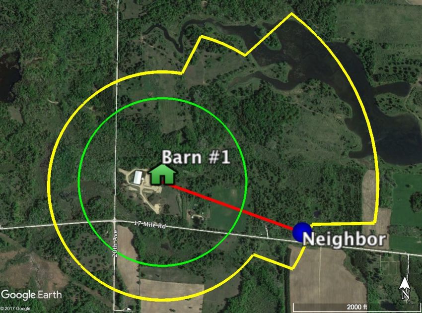
• Overlaying the odor footprint generated by MI OFFSET 2000 on maps of neighbors, roads,
local communities, etc., is an important part of the siting process, but requires the user to
export the footprint image from the Excel spreadsheet and overlay it on a static map or in GIS
software (e.g., Google Earth). This is a cumbersome and inherently error-prone procedure.
4. MI OFFSET 2018
4.1. Background
A project to update the Siting GAAMP document (discussed in section 3.1), funded by the
Michigan Alliance for Animal Agriculture (M-AAA), was begun in early 2016. One of the primary
tasks outlined in the funded proposal was, to quote the proposal, the ”Development of a user
interface that, via input data, incorporates local and current historical meteorological data for site-
specific odor footprint development”. In other words, the project called for (1) replacing the EPA-
SCRAM dataset of wind and stability with a dataset that accounts for differences in wind and
stability climatologies across the state, and (2) developing an interface to allow a user to enter the
location of their livestock facility and obtain siting guidance that takes into account the local wind
and stability climatology. The product of these efforts is MI OFFSET 2018.
174.2. Updated wind and atmospheric stability climatology
4.2.1) I NTRODUCTION TO NARR
Figure 5: NARR daily mean temperature for April 11, 1979. Data are plotted on a Lambert Conformal
projection. The values are the mean of eight 3-hourly values. (Climate Data Guide; D. Shea)
The North American Regional Reanalysis (NARR) meteorological gridded dataset (Mesinger
et al. 2006) was chosen to replace the EPA-SCRAM 1984-1992 dataset. NARR is a three-dimensional
gridded dataset that combines forecasts from a weather model [that resolves or in some way ac-
counts for physical processes (e.g., boundary layer processes like turbulent mixing)], and ground
truth from a suite of atmospheric observations. The NARR domain, as it’s name suggests, cov-
ers all of North America and surrounding waters (Fig. 5). NARR was chosen to replace the
EPA-SCRAM dataset for several reasons. First, NARR is able to characterize lake-modified wind
and stability climatologies. NARR provides weather data on a regular 32-km grid, with the spac-
ing between adjacent grid points smaller than the average spacing of weather stations capable of
providing the information required for calculation of Pasquill stability class. Second, the NARR
period of record begins on 1 January 1979, affording a much longer dataset than was available for
the development of MN OFFSET and MI OFFSET 2000. A longer period of record minimizes
the impact of any single year on statistics computed from the dataset, reducing the risk of bias
from one or two unrepresentative years (for example, the anomalously warm 1988). For the devel-
opment of MI OFFSET 2018, the 30-year period from 1 January 1979 – 31 December 2008 was
chosen. Third, NARR provides a larger suite of variables with which to work with, relative to the
EPA-SCRAM dataset. This allows for the use of other methods of determining Pasquill stability
class than the 10-m wind speed / solar insolation / cloud cover method used in previous versions
of OFFSET, methods that in some cases have a more solid physical basis (section 4.2.3).
184.2.2) NARR WIND ASSESSMENT AND WIND SPEED ADJUSTMENT
Due to the expected sensitivity of odor plume dispersion to wind, both directly through speed
and direction, and indirectly via atmospheric stability, an assessment of NARR wind speed and
direction was performed as a preliminary step in the development of MI OFFSET 2018. For this
assessment, ten years of hourly observations [1 Jan 1999 – 31 Dec 2008] were obtained from eight
automated weather stations (Table 3).
Table 3: Metadata for eight automated weather stations used in NARR wind assessment.
Station ID Name Latitude [deg N] Longitude [deg W]
KANJ Sault St. Marie 46.48 84.37
KAPN Alpena 45.08 83.56
KDTW Detroit 42.21 83.35
KGRR Grand Rapids 42.89 85.52
KLAN Lansing 42.78 84.59
KMBS Saginaw 43.53 84.08
KSBN South Bend, IN 41.71 86.32
KTVC Traverse City 44.74 85.58
After pooling the data from the eight stations, and isolating every third hourly observation,
to match the three-hourly NARR interval, the NARR and station wind speeds were compared in
a scatter plot (Fig. 6). Before proceeding, two points of clarification are necessary. First, it is
important to keep in mind that we are comparing area-average estimates to point observations
and an unknown portion of the differences between the station observations and gridded estimates
quoted herein can be attributed to spatial variability occurring at scales too small to be resolved by
the 32-km grid. Second, analysis of the individual stations (not shown) revealed differences in the
accuracy of NARR estimates between stations that are well inland (e.g., KLAN) and stations that
are closer to the lakeshore (e.g., KTVC): accuracy is greatest at locations well inland and lowest
at locations in closer proximity to the lakeshore. That said, pooling of the data was performed
in the interest of generalizing the accuracy assessment and creating a one-size-fits-all wind speed
adjustment.
19Figure 6: Scatter plot of NARR estimated and observed wind speed [m s−1 ], for eight stations identified in
text. Statistics are overlaid on plot: N (number of data points); M (mean difference); R (root mean square
difference); C (correlation coefficient); S (slope). Dashed line is the 1:1 line, and the thick line is the least
squares fit (linear regression equation included).
As seen in Fig. 6, considerable random error in the NARR estimates are apparent, with a
root mean square difference of 2.11 m s−1 . This is in part attributable to the comparison of area-
average estimates to point observations. The mean difference (station-NARR) of -0.82 m s−1
indicates a general tendency for NARR to overestimate wind speeds. Notably, the least squares fit
line intersects the 1:1 line at about 2 m s−1 , showing that NARR wind speed less than about 2 m
s−1 actually tend to be too weak, with NARR wind speeds above 2 m s−1 tending to be too strong.
The corresponding linear regression equation [0.65198x + 0.77577] was subsequently applied to
the NARR wind speed at every grid point, over the entire 30-year dataset.
Following the adjustment of the NARR wind speed, comparison of NARR estimates and indi-
vidual station observations was made with both the adjusted and original NARR estimates (Table
4). The eight-station-median mean difference before and after the adjustment is 0.69 and -0.08
m s−1 , respectively. Keeping in mind that this assessment was performed with the same eight sta-
tions used in developing the regression equation, the reduction in overall mean difference increases
confidence in the use of NARR for the MI OFFSET 2018 tool.
Table 4: Wind speed mean difference (NARR-station), before and after wind speed adjustment, along with
eight-station median of the difference.
Mean difference KANJ KAPN KDTW KGRR KLAN KMBS KSBN KTVC Eight-station
[m s−1 ] median
Before 1.94 -0.20 0.54 0.19 0.84 1.83 1.23 0.20 0.69
After 0.96 -0.85 -0.26 -0.53 0.10 0.79 0.15 -0.59 -0.08
204.2.3) S ELECTION OF METHOD FOR ESTIMATING PASQUILL CLASS
Methods for estimating Pasquill stability class may be grouped into three broad categories,
those that have a weak physical basis, but are readily computed from standard station data (10-m
wind speed / solar insolation / cloud cover method), those that have a somewhat greater physi-
cal basis but that require measurements not typically available from station data (standard devia-
tion of wind direction fluctuation method, vertical temperature gradient method, wind speed ratio
method), and those that are most complete in their physical basis but are generally too complicated
and too restrictive in their requirements to be computed from station data [Obukhov length method,
flux Richardson number (RiF) method]. We restrict discussion in this document to the last group;
for information about the other methods, see Mohan and Siddiqui (1998).
The two methods with the strongest physical basis are similar in that they compare the relative
roles of shear and buoyancy in the production and/or consumption of turbulent kinetic energy
(TKE). TKE is the mean kinetic energy per unit mass associated with eddies in turbulent flow, and
is a useful metric for evaluating the ability of the atmosphere to mix fresh air into the plume of
pollutants emanating from a source, thus diluting the plume. Knowledge of the propensity of the
atmosphere to favor or oppose the development of turbulence within the planetary boundary layer
is the motivating factor for using such methods to diagnose Pasquill stability class. Ordinarily, such
methods are difficult to apply in practice as they require variables or quantities not easily obtained
from standard surface observations, and are too complicated for rapid calculations. However, the
use of a dataset like NARR allows for the potential application of such methods. The RiF method
was chosen for this project based on the availability of a NARR-derived RiF dataset (section 4.2.4).
4.2.4) NARR- BASED PASQUILL CLASS : M ETHODOLOGY
The NARR-based RiF dataset was developed as part of a climatological study of turbulent con-
ditions favoring erratic fire spread (Heilman and Bian 2013). The authors of that study graciously
offered to make their dataset available to our group.
The form of RiF used in Heilman and Bian (2013) is expressed as
−g 0 0
θ
w θ kzθ
RiF = 3 (2)
kU
10
where g is gravitational acceleration [m s−2 ], θ is the mean potential temperature [K], kzθ is
the height above ground level at which θ is valid [m], w0 θ0 is sensible heatflux [K m s−1 ], U is the
mean wind speed [m s−1 ], and k is the Von-Karman constant [0.35-0.4; dimensionless] (X. Bian,
personal communication). The denominator in Eq. (2) is always a production term, representing
the conversion of kinetic energy of the mean flow to turbulent kinetic energy. The numerator in
Eq. (2) can be either a production (mostly daytime) or consumption (mostly nighttime) term. The
relative strength of shear and buoyancy, as well as the sign of the buoyancy term itself, determine
whether turbulent kinetic energy will increase, decrease, or remain steady.
To compute RiF from NARR, X. Bian developed a routine that takes three NARR variables as
input: 2-m potential temperature (θ) surface sensible heat flux (w0 θ0 ), and 10-m wind speed (U ).
21The dataset was provided by X. Bian in the form of text files, covering the entire NARR North
American domain, and the full 30-year period (1979-2008). After obtaining the dataset, a routine
was developed to convert the text files into a compressed and more portable data format: HDF-5.
In additional to the vast compression advantage of HDF-5 over plain text files, use of HDF-5 files
enables efficient I/O for use with the on-demand footprint tool (section 4.4).
Finally, an empirical relationship was used to assign Pasquill stability class based on the NARR
RiF value (Table 5). The relationship was developed by Mohan and Siddiqui (1998) based on
observations collected during a 2-year field campaign at a coal-fired power plant near Kincaid, IL.
Table 5: RiF limits for Pasquill classification, adapted from Table 7 in Mohan and Siddiqui (1998).
Pasquill stability class Flux Richardson number
A RiF ≤ -5.34
B -5.34 ≤ RiF < -2.26
C -2.26 ≤ RiF < -0.569
D -0.569 ≤ RiF < 0.083
E 0.083 ≤ RiF < 0.196
F RiF >= 0.196
4.2.5) NARR- BASED PASQUILL CLASS : E VALUATION
Unfortunately, no validation of the NARR RiF dataset was performed in Heilman and Bian
(2013). Thus, before proceeding further, an evaluation of the NARR RiF-derived Pasquill class
dataset was performed. Note that the use of the sensible heat flux in the RiF formulation [Eq.
(2)] necessitated the use of flux tower measurements. Tower measurements at four AmeriFlux
(http://ameriflux.lbl.gov/) tower sites were used for this exercise. The AmeriFlux network is a
community of sites and scientists measuring ecosystem carbon, water, and energy fluxes across the
Americas, and committed to producing and sharing high quality eddy covariance data (AmeriFlux
mission statement). The four stations were chosen based on two factors: period of record, and
a desire to consider both cropland and grassland sites. Metadata for the four sites is provided in
Table 6.
Table 6: Metadata for four AmeriFlux micrometeorological towers used in the NARR RiF-derived Pasquill
class assessment. The last three columns indicate the height above the ground at which potential temperature
(θ), sensible heat flux (w0 θ0 ), and wind speed (U ) were measured.
Identifier Location Start End Land Use % miss θ w0 θ0 U
ARM Lamont, OK 00Z 1/1/01 21Z 12/31/08 Cropland 44 2.15 4.28 4.28
Bo1 Bondvile, IL 21Z 8/25/96 18Z 4/8/08 Cropland 16 10 10 10
IB1 Batavia, IL 00Z 3/29/05 21Z 12/31/08 Cropland 14 4.05 4.05 4.05
SdH Whitman, NE 06Z 1/1/04 21Z 12/31/08 Grassland 41 1.92 3.85 3.8
For each tower, Pasquill class was determined from the tower and NARR-based RiF time series
using Table 5. The frequencies of the D, E, and F stability classes, as well as the combined
22unstable A-C classes, were computed from the tower data and NARR; the Pasquill class frequency
distributions are presented in Fig. 7. Overall, the comparison is mixed, but acceptable, with the
poorest comparison at the two plains sites (ARM and SdH). At ARM, NARR overestimates class
F frequency by 10% and underestimates class D frequency by just over 50%, and at SdH, NARR
overestimates slightly the frequency of class F but underestimates class D by 40%. At the two
Illinois towers (Bo1 and IB1), the comparison is better, lending confidence to the use of NARR
RiF at sites in nearby Michigan. The climate of Michigan shares arguably more in common with
Illinois than the central or southern Plains states.
Figure 7: Frequency of Pasquill classes D, E, and F, used in OFFSET, along with the frequency of the
unstable classes (A-C), at four AmeriFlux towers. Top panels are based on observed conditions, and the
bottom panels are derived from NARR (with wind speed bias-correction applied).
23Supplemental: Evaluation of Methods for Selection of 1.5%, 3%, and 5% Classes
In developing the new version of MI OFFSET, the three odor-annoyance frequencies selected
in MI OFFSET 2000 were retained, as well as the method of picking the wind-stability class
whose frequency came closest, without going over, to the particular odor-annoyance fre-
quency. As discussed in section 3.3 (Supplemental: Odor-annoyance class - wind-stability
climatology relationship), this is an inherently conservative method.
As an experiment, an alternate method was examined wherein the wind-stability class whose
frequency came closest to the odor annoyance frequency (regardless of overestimate or
underestimate) was chosen. The results of this experiment are presented in Fig. 8, wherein
the 1.5% and 5% footprints at all 142 NARR grid points in Michigan are visualized in
Google Earth using an arbitrarily large total odor emission factor, and in Table 7 using
a total odor emission factor of 108. Overall, the area of the footprint is smaller with the
alternate method (colored outlines in Fig. 8) versus the original methodology (white outlines
in Fig. 8). In other words, the alternate method is less conservative with smaller setback
distances. The greatest sensitivity to the choice of method occurs for the 1.5% footprint, and
the weakest sensitivity occurs for the 5% footprint.
Based on a comparison of 142-grid-point-median footprint area and maximum setback dis-
tance, differences between the two methods are negligible for the 5% footprint (last two
columns in Table 7). Note that the percent differences between the two methods are unaf-
fected by use of a larger total odor emission factor (not shown). A decision was made to
use the original MI OFFSET 2000 method, based on three factors: (1) differences in the 5%
footprints generated between the original and alternate methods were negligible, (2) the ex-
isting method is the more conservative approach, and (3) by retaining the MI OFFSET 2000
method, continuity is maintained between MI OFFSET 2000 and 2018.
24Evaluation of Methods for Selection of 1.5%, 3%, and 5% Classes (continued)
Figure 8: Google Earth overview of footprints at all 142 NARR grid points in Michigan. White lines
indicate footprint generated using the MI OFFSET 2000 method for determining the (a) 1.5% and
(b) 5% footprints (closest to without going over). Colored lines indicate footprint generated using
an alternate approach in which the wind-stability class that came closest to the odor-annoyance
frequency was chosen, regardless of over- or underestimation. Note: for this visualization, a very
large total odor emission factor was used. Thus, the absolute setback distances do not have physical
meaning.
25Evaluation of Methods for Selection of 1.5%, 3%, and 5% Classes (continued)
Table 7: Comparison of 142-grid-point-median footprint area and maximum setback distance be-
tween footprints generated using the MI OFFSET 2000 “closest to without going over” approach to
choosing wind-stability class, and an alternate method of choosing the wind-stability class wherein
the wind-stability class that comes closest to the odor-annoyance frequency, regardless of over- or
underestimation, is chosen. For this table, a total odor emission factor of 108 was used. Note that
the percent differences between the two methods are unaffected by use of a larger total odor emission
factor.
Method 1.5% 1.5% median 3% 3% median 5% 5% median
median maximum median maximum median maximum
footprint setback footprint setback footprint setback
area distance area distance area distance
Closest, 4.76 1.31 0.56 0.50 0.28 0.27
without
going
over
Closest, 2.18 0.78 0.46 0.37 0.25 0.27
either
over or
under
4.3. Construction of odor footprint
The odor footprint is generated by MI OFFSET 2018 based on odor source information and
source location provided by the user. The underlying program takes as input the source location,
determines the closest NARR grid point, constructs a 30-year climatology of wind and atmospheric
stability at the NARR grid point, and, as in MI OFFSET 2000, generates a 3 x 16 table of wind
stability-class [3 odor-annoyance frequencies and 16 wind direction bins]. However, unlike MI
OFFSET 2000, this table is location-specific rather than one-size-fits-all. At this point in the pro-
gram, the steps are identical to that of MI OFFSET 2000. Based on the total odor emission factor
(E) computed from the user-provided odor source information, the setback distance is computed
for each element in the 3x16 table, using the a and b coefficients from MN OFFSET, and E.
Finally, lines are drawn connecting the setback distances to create the three footprints.
4.4. On-demand odor footprint tool
4.4.1) T RANSITION FROM M ICROSOFT E XCEL SPREADSHEET TO WEB TOOL
In transitioning from MI OFFSET 2000, a one-size-fits-all tool, to MI OFFSET 2018, a location-
specific tool, a decision was made to terminate use of the Microsoft Excel platform. This decision
was made for a number of reasons. First and foremost, the location-specific nature makes the use of
26You can also read