Prediction of source contributions to urban background PM10 concentrations in European cities: a case study for an episode in December 2016 using ...
←
→
Page content transcription
If your browser does not render page correctly, please read the page content below
Geosci. Model Dev., 13, 1787–1807, 2020
https://doi.org/10.5194/gmd-13-1787-2020
© Author(s) 2020. This work is distributed under
the Creative Commons Attribution 4.0 License.

Prediction of source contributions to urban background PM10
concentrations in European cities: a case study for an episode in
December 2016 using EMEP/MSC-W rv4.15 and LOTOS-EUROS
v2.0 – Part 1: The country contributions
Matthieu Pommier1 , Hilde Fagerli1 , Michael Schulz1 , Alvaro Valdebenito1 , Richard Kranenburg2 , and
Martijn Schaap2,3
1 Norwegian Meteorological Institute, Oslo, Norway
2 TNO, P.O. Box 80015, 3508TA Utrecht, the Netherlands
3 FUB – Free University Berlin, Institut für Meteorologie, Carl-Heinrich-Becker-Weg 6–10, 12165 Berlin, Germany

Correspondence: Matthieu Pommier (matthieu.pommier@met.no)

Received: 2 April 2019 – Discussion started: 28 May 2019
Revised: 24 January 2020 – Accepted: 2 March 2020 – Published: 3 April 2020

Abstract. A large fraction of the urban population in Europe      then it is compared to a reference run where no changes are
is exposed to particulate matter levels above the WHO guide-      applied. Different percentages (5 %, 15 %, and 50 %) for the
line value. To make more effective mitigation strategies, it is   reduced emissions in the EMEP/MSC-W model were used
important to understand the influence on particulate matter       to test the robustness of the methodology. The impact of the
(PM) from pollutants emitted in different European nations.       different ways to define the urban area for the studied cities
In this study, we evaluate a country source contribution fore-    was also investigated (i.e. one model grid cell, nine grid cells,
casting system aimed at assessing the domestic and trans-         and grid cells covering the definition given by the Global Ad-
boundary contributions to PM in major European cities for an      ministrative Areas – GADM). We found that the combination
episode in December 2016. The system is composed of two           of a 15 % emission reduction and a larger domain (nine grid
models (EMEP/MSC-W rv4.15 and LOTOS-EUROS v2.0),                  cells or GADM) helps to preserve the linearity between emis-
which allows the consideration of differences in the source       sion and concentrations changes. The nonlinearity, related to
attribution.                                                      the emission reduction scenario used, is suggested by the na-
   We also compared the PM10 concentrations, and both             ture of the mismatch between the total concentration and the
models present satisfactory agreement in the 4 d forecasts of     sum of the concentrations from different calculated sources.
the surface concentrations, since the hourly concentrations       Even limited, this nonlinearity is observed in the NO−        +
                                                                                                                         3 , NH4 ,
can be highly correlated with in situ observations. The cor-      and H2 O concentrations, which is related to gas–aerosol par-
relation coefficients reach values of up to 0.58 for LOTOS-       titioning of the species. The use of a 15 % emission reduction
EUROS and 0.50 for EMEP for the urban stations; the values        and of a larger city domain also causes better agreement on
are 0.58 for LOTOS-EUROS and 0.72 for EMEP for the ru-            the determination of the main country contributors between
ral stations. However, the models underpredict the highest        both country source calculations.
hourly concentrations measured by the urban stations (mean            Over the 34 European cities investigated, PM10 was domi-
underestimation of 36 %), which is to be expected given the       nated by domestic emissions for the studied episode (1–9 De-
relatively coarse model resolution used (0.25◦ longitude ×        cember 2016). The two models generally agree on the domi-
0.125◦ latitude).                                                 nant external country contributor (68 % on an hourly basis) to
   For the source attribution calculations, LOTOS-EUROS           PM10 concentrations. Overall, 75 % of the hourly predicted
uses a labelling technique, while the EMEP/MSC-W model            PM10 concentrations of both models have the same top five
uses a scenario having reduced anthropogenic emissions, and       main country contributors. Better agreement on the dominant

Published by Copernicus Publications on behalf of the European Geosciences Union.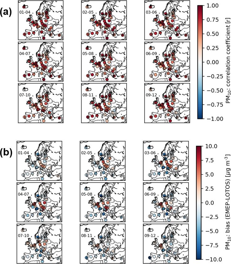
1788                     M. Pommier et al.: Prediction of source contributions to PM10 concentrations in European cities

country contributor for primary (emitted) species (70 % is         of forest fires, mineral dust, and sea salt. The main sink is
found for primary organic matter (POM) and 80 % for ele-           the wet deposition. The dry deposition can also be important
mental carbon – EC) than for the inorganic secondary com-          and depends on the type of land surface such as grass, tree
ponent of the aerosol (50 %), which is predictable due to the      leaves, and others and on meteorological conditions. With
conceptual differences in the source attribution used by both      these components being derived from various sources, we
models. The country contribution calculated by the scenario        understand the importance of reflecting properly the source
approach depends on the chemical regime, which largely im-         contributions while using modelling for policy support.
pacts the secondary components, unlike the calculation using          Many studies have already focused on source–receptor re-
the labelling approach.                                            lationships to calculate the transport of atmospheric pollu-
                                                                   tants, with country-to-country relationships (e.g. EMEP Sta-
                                                                   tus Report, 2018) but also over cities (e.g. Thunis et al.,
                                                                   2016, 2018). However, these studies focus on annual means,
1   Introduction                                                   whereas information is also required on exposure from
                                                                   episodes which cause short-term limit value exceedances
The adverse health impacts from air pollution and especially       throughout Europe. Source apportionment provides valuable
from particulate matter (PM) are a well-documented prob-           information on the attribution of different sources to PM10
lem (e.g. Keuken et al., 2011; REVIHAAP, 2013; Mukherjee           concentrations. A country source calculation allows us to
and Agrawal, 2017; Segersson et al., 2017). Furthermore, it        tackle the emissions from the countries responsible for the
affects crop yields (e.g. Crippa et al., 2016), visibility (e.g.   air pollution episode. Two distinct methodologies have been
Founda et al., 2016) and even the economy (e.g. Meyer and          compared in this study. Indeed, the country source contribu-
Pagel, 2017). The mass of particulate matter with an aero-         tion presented hereafter is performed by two regional mod-
dynamic diameter lower than 10 µm (PM10 ) is an air qual-          els, the EMEP/MSC-W model (Simpson et al., 2012) and
ity metric linked to premature mortality at high exposure          LOTOS-EUROS (Manders et al., 2017).
(e.g. Dockery and Pope, 1994). The World Health Organi-               The EMEP calculations use a reduced anthropogenic
zation (WHO) has established a short-term exposure PM10            emission scenario and compare it to a reference run where
guideline value of 50 µg m−3 daily mean that should not be         no changes are applied. It is also known as the scenario ap-
exceeded in order to ensure healthy conditions (the long-          proach. With such a simulation comparison, the simulation
term exposure guideline is 20 µg m−3 for annual mean PM10 )        with reduced emissions over a source region (e.g. a coun-
(WHO, 2005). Although policies have been proposed and              try) allows us to highlight the impact of this source on the
implemented at the international (e.g. Amann et al., 2011)         concentrations over a receptor, hereafter a city. Hence, the
and national (e.g. D’Elia et al., 2009) levels, European cities    scenario approach is useful for analysing the concentration
still suffer from poor air quality (EEA report, 2017), espe-       changes due to emission reductions. On the other hand, one
cially due to high PM10 concentrations. In short, to further       simulation per source is needed to calculate the impact of
decrease the adverse health impacts of PM in Europe, its con-      each source, as is done on annual means for each country
centrations need to be reduced further.                            in each EMEP report (e.g. EMEP Status Report, 2018). The
   PM10 concentrations in the atmosphere are highly variable       scenario approach may also lead to a nonlinearity in the cal-
in space and time. Due to the relative short atmospheric life      culated concentrations, i.e. a slight difference between the
time (from some hours to days), the variability is impacted        concentrations over a receptor and the sum of the estimated
by local sources, meteorological conditions affecting disper-      concentrations from different sources over this same recep-
sion, and long-range transport as well as chemical regimes         tor, as shown by Clappier et al. (2017a). Thus, the scenario
controlling the efficiency of secondary formation. PM10 con-       approach is more appropriate for the calculation of the source
sists of both primary and secondary components. Primary            contribution of the primary PM components than for nonlin-
PM10 components include organic matter (OM), elemental             ear species such as the secondary components (e.g. Burr and
carbon (EC), dust, sea salt (SS), and other compounds. Sec-        Zhang, 2011; Thunis et al., 2019). LOTOS-EUROS traces
ondary PM10 is comprised of compounds formed by chem-              the origin of air pollutants throughout a simulation using a la-
ical reactions in the atmosphere from gas-phase precursors.        belling approach. The advantage of the labelling technique is
This includes various compounds such as nitrate (NO−    3 ) from   the reduction in the computational time, in comparison with
nitrogen oxide (NOx ) emissions, ammonium (NH+         4 ) from    the scenario approach. It also quantifies the contribution of
ammonia (NH3 ) emissions, sulfate (SO2−   4 ) from sulfur  diox-   an emission source to the concentration of one pollutant at
ide (SO2 ) emissions, and a large range of secondary organic       one given location. However, it is not designed to study the
aerosol (SOA) compounds from both anthropogenic and bio-           impact of emission abatement policies on pollutants concen-
genic volatile organic compounds (VOCs). The sources for           trations (Grewe et al., 2010; Clappier et al., 2017b), and only
PM and its precursors are numerous, but the main anthro-           traceable atoms can be used in labelling approach, i.e. only
pogenic sources are the transport, industries, energy produc-      conserved atoms (C, N, and S), directly related to emission
tion, and agriculture. The main natural sources are composed       sources, in their different oxidation states. Thus, for exam-

Geosci. Model Dev., 13, 1787–1807, 2020                                              www.geosci-model-dev.net/13/1787/2020/
M. Pommier et al.: Prediction of source contributions to PM10 concentrations in European cities                                 1789

ple, the origin of ozone (O3 ) cannot be studied, which can            tributions of emissions from different countries in each city
be done with the scenario approach. Even if both method-               (Fig. 1).
ologies mainly aim to answer two different questions, i.e.                The system is composed of predictions from two re-
the emission control scenarios with the scenario approach              gional models (the EMEP/MSC-W model and LOTOS-
and the attribution of concentrations from a source by the la-         EUROS), using two distinct source contribution calcula-
belling technique, it is still useful to estimate the reliability of   tion methodologies. The EMEP/MSC-W chemistry transport
both methodologies in the estimation of the source contribu-           model (Simpson et al., 2012) has been used for decades
tion to PM10 concentrations. For example, it is important to           to calculate source–receptor relationships between European
ensure that the nonlinearity, related to the perturbation used         countries (and Russia) (e.g. EMEP Status Report, 2018), and
in the scenario approach, has a limited impact on the calcu-           the LOTOS-EUROS chemistry transport model (Manders et
lated contributions and to show that both methodologies may            al., 2017) has also been used in several source apportionment
present similar results in the country source attribution.             studies over Europe, especially for PM (Hendriks et al., 2013,
   Both models are part of the operational country source              2016; Schaap et al., 2013). Both models are involved in the
contribution (SC) prediction system for the European cities            operational air quality analysis and forecasting for Europe in
within the Copernicus Atmosphere Monitoring Service                    the CAMS regional ensemble system (Marécal et al., 2015)
(CAMS). This system aims at attributing country contribu-              and for China (Brasseur et al., 2019). For the simplicity of
tion to surface PM10 in European cities for 4 d forecasts. The         the reading, the EMEP/MSC-W model is hereafter referred
objective of this study is to evaluate the robustness of a new         to as the EMEP model.
system that provides forecasts of source-region-resolved PM               Both models are Eulerian models, but there are differences
for European cities. The evaluation of the system is focused           between these two models such as the calculation of the plan-
on an event occurring between 1 and 9 December 2016,                   etary boundary layer (PBL) and of the advection, the vertical
which corresponds to the first event listed from the beginning         resolution. There are also differences, which include the fol-
of the development of our system. To do so, the predicted              lowing: the presence of the secondary organic aerosol (in-
PM10 concentrations are compared with observations. The                cluded in the EMEP model and not in LOTOS-EUROS),
simulations from both models, for the concentrations and the           the PM10 diagnosing particle water explicitly in the EMEP
SC calculations, are also intercompared.                               model and not in LOTOS-EUROS, the calculation of the bio-
   Section 2 describes the country SC system composed of               genic emissions, the description of the gas-phase chemistry,
the two models and the experiment. Section 3 describes the             and the treatment of dust (from agriculture and traffic are in-
studied episode, and it presents the evaluation of both pre-           cluded in LOTOS-EUROS and not in the EMEP model).
dictions in terms of PM10 concentrations. The methodology                 The main details about the models and the experiment are
used for the SC calculations by both models is explained in            provided in the Table 1, and a more complete description is
Sect. 4. Then Sect. 5 gives an overview of the composition             provided in the following sections.
and the origin of PM10 over the cities predicted by both mod-
els and the issue regarding the nonlinearity in the chemistry          2.2   Description of the EMEP model
related to the EMEP SC calculation. Section 6 is a compar-
ison between the two country SC calculations. Finally, the             The EMEP model is a 3D Eulerian chemistry-transport
conclusions are provided in Sect. 7.                                   model described in detail in Simpson et al. (2012). Initially,
                                                                       the model has been aimed at European simulations, but the
                                                                       model has also been used over other regions and at global
                                                                       scale for many years (e.g. Jonson et al., 2010). The EMEP
2     Description of the country source apportionment
                                                                       model version rv4.15 has been used here in the forecast
      system
                                                                       mode. The version rv4.15 has been described in Simpson
2.1    Overview of the system                                          et al. (2017) and references cited therein. The main updates
                                                                       since Simpson et al. (2012), used in this work, concern a new
Within CAMS, a country SC product has been developed.                  calculation of aerosol surface area (now based upon the semi-
This is a new forecasting and near-real-time source alloca-            empirical scheme of Gerber, 1985), revised parameteriza-
tion system for surface PM10 concentrations and its different          tions of N2 O5 hydrolysis on aerosols, additional gas–aerosol
components over all European capitals. The predictions are             loss processes for O3 , HNO3 , and HO2 , a new scheme for
available online at https://policy.atmosphere.copernicus.eu/           ship NOx emissions, a new calculated natural marine emis-
SourceContribution.php (last access: 24 January 2020). The             sions of dimethyl sulfide (DMS), and the use of a new land
concentrations are calculated over the 28 EU capitals plus             cover (used to calculate biogenic VOC emissions and the dry
Bern, Oslo, and Reykjavik. Forecasts for Barcelona, Rotter-            deposition) (Simpson et al., 2017). This version is the offi-
dam, and Zurich are also provided. In addition to providing            cial EMEP Open Source version that was released in Septem-
information about the air quality over the selected cities by          ber 2017 (Table 1).
focusing on PM10 , this product aims at quantifying the con-

www.geosci-model-dev.net/13/1787/2020/                                                   Geosci. Model Dev., 13, 1787–1807, 2020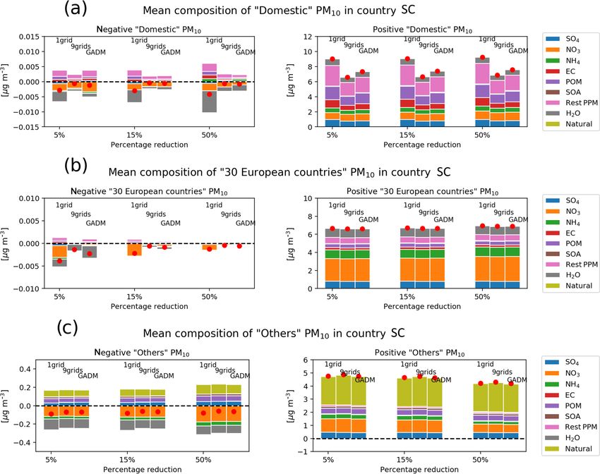
1790                        M. Pommier et al.: Prediction of source contributions to PM10 concentrations in European cities

Table 1. Technical description of both models used in the SC calculation system.

    Model                            EMEP/MSC-W                                         LOTOS-EUROS
    Model version                    rv4.15 (open-source version September 2017)        V2.0 (open-source version 2016)
    Horizontal resolution            0.25◦ × 0.125◦ long–lat                            0.25◦ × 0.125◦ long–lat
    Regional domain                  30–76◦ N                                           31–68.875◦ N
                                     30◦ W–45◦ E                                        24◦ W–43.75◦ E
    PBL                              Calculation based on turbulent diffusion coeffi-   From ECMWF
                                     cients (Kz) (EMEP Status Report 1/2003)
    Vertical resolution              20 sigma layers up to 100 hPa, with about 10       Mixing layer approach with a 25 m surface
                                     in the planetary boundary layer                    layer; model top at 5 km.
    Gas phase chemistry              Evolution of the “EMEP scheme” (Andersson-         TNO-CBM-IV (Schaap et al., 2009)
                                     Sköld and Simpson, 1999; Simpson et al., 2012)
    Nitrate formation                Oxidation of NO2 by O3 on aerosols                 N2 O5 hydrolysis on aerosol
                                     (night and winter)                                 (Schaap et al., 2004)
                                     N2 O5 hydrolysis on aerosol
                                     (Simpson et al., 2012)
    Sulfate production               SO2 oxidation by O3 and H2 O2                      SO2 oxidation by O3 and H2 O2
    Inorganic aerosols               MARS (Binkowski and Shankar, 1995)                 ISORROPIA II (Fountoukis and Nenes, 2007)
    Secondary organic aerosols       EmChem09soa (Bergström et al, 2012)                Not included in this model version
    Water                            PM10 particle water at 50 % relative humidity      Not diagnosed
    Advection                        Scheme of Bott (1989)                              Monotonic advection scheme
                                                                                        (Walceck and Aleksic, 1998)
    Dry deposition/sedimentation     Resistance approach for gases and for aerosol,     Resistance approach for gases and for aerosol,
                                     including nonstomatal deposition of NH3            including compensation point for NH3
                                     (EMEP Status Report 1/2003)                        (van Zanten et al., 2011; Wichnik Kuit et al.,
                                                                                        2012; Zhang et al., 2001)
    Wet deposition                   Washout ratio                                      pH-dependent washout ratio accounting for
                                                                                        saturation
    Dust                             Boundary conditions + windblown dust               Boundary conditions + soil, traffic, and agricul-
                                                                                        ture (Schaap et al., 2009)
    Sea salt                         Mårtensson et al. (2003), Monahan et al. (1986)    Mårtensson et al. (2003), Monahan et al. (1986)
                                     production accounting for whitecap area frac-
                                     tions (Callaghan et al., 2008)
    Boundary values                  Global C-IFS 00:00 UTC                             Global C-IFS 00:00 UTC, except for sea salt
    Initial values                   24 h forecast from the day before                  24 h forecast from the day before
    Anthropogenic emissions          TNO-MACC-III for 2011                              TNO-MACC-III for 2011
    Fire emissions                   CAMS product: GFAS                                 CAMS product: GFAS
    Biogenic emissions               Emission factors as a function of temperature      Emission factors as a function of temperature
                                     and solar radiation (Simpson et al., 2012)         and solar radiation (Schaap et al., 2009)
    Meteorological driver            12:00 UTC operational IFS forecast                 12:00 UTC operational IFS forecast
                                     (previous day’s)                                   (previous day’s)

Geosci. Model Dev., 13, 1787–1807, 2020                                                    www.geosci-model-dev.net/13/1787/2020/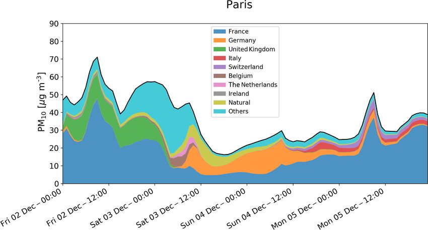
M. Pommier et al.: Prediction of source contributions to PM10 concentrations in European cities                                     1791

Figure 1. Hourly PM10 concentrations, in micrograms per cubic metre, over Paris predicted by the EMEP model from 2 to 5 December 2016.
The black curve highlights the total concentration. The eight main country contributors are plotted in addition to the natural sources and
“Others”. Others contains hereafter other European countries, boundary conditions, ship traffic, biogenic sources, aircraft emissions, and
lightning.

   Vertically, the model uses 20 levels defined as sigma coor-         scheme detailed in Bergström et al. (2012) and Simpson et
dinates (Simpson et al., 2012). The PBL is located within ap-          al. (2012).
proximately the 10 lowest model levels (∼ five levels below               The main loss process for particles is wet-deposition, and
500 m), and the top of the model domain is at 100 hPa. The             the model calculates in-cloud and subcloud scavenging of
PBL height is calculated based on the turbulent diffusivity            gases and particles as detailed in Simpson et al. (2012). Wet
coefficient as described in the EMEP Status Report (2003).             scavenging is treated with simple scavenging ratios, taking
The numerical solution of the advection terms is based upon            into account in-cloud and subcloud processes.
the scheme of Bott (1989).                                                In the EMEP model, the 3D precipitation is needed. An es-
   The chemical scheme couples the sulfur and nitrogen                 timation of this 3D precipitation can be calculated by EMEP
chemistry with the photochemistry using about 140 reactions            if this parameter is missing in the meteorological fields as
between 70 species (Andersson-Sköld and Simpson, 1999;                 in the data used in this work (see Sect. 2.4). This estimate
Simpson et al., 2012). The chemical mechanism is based on              is derived from large-scale precipitation and convective pre-
the “EMEP scheme” described in Simpson et al. (2012) and               cipitation. The height of the precipitation is derived from the
references therein.                                                    cloud water. Then, it is defined as the highest altitude above
   The biogenic emissions of isoprene and monoterpene are              the lowest level, at which the cloud water is larger than a
calculated in the model by emission factors as a function of           threshold taken as 1.0 × 10⁻⁷ kg water per kg air. Precipita-
temperature and solar radiation (Simpson et al., 2012). The            tions are only defined in areas where surface precipitations
soil-NO emissions of seminatural ecosystems are specified              occur. The intensity of the precipitation is assumed constant
as a function of the N deposition and temperature (Simpson             over all heights where they are nonzero
et al., 2012). The biogenic DMS emissions are calculated dy-              Gas and particle species are also removed from the atmo-
namically during the model calculation and vary with the me-           sphere by dry deposition. This dry deposition parameteriza-
teorological conditions (Simpson et al., 2016).                        tion follows standard resistance formulations, accounting for
   PM emissions are split into EC, OM (here assumed in-                diffusion, impaction, interception, and sedimentation.
ert), and the rest of primary PM defined as the remainder, for
both fine and coarse PM. The OM emissions are further di-              2.3   Description of LOTOS-EUROS
vided into fossil-fuel and wood-burning compounds for each
source sector. As in Bergström et al. (2012), the OM / OC              The LOTOS-EUROS model is an offline Eulerian chemistry-
ratios of emissions by mass are assumed to be 1.3 for fossil-          transport model which simulates air pollution concentrations
fuel sources and 1.7 for wood-burning sources. The model               in the lower troposphere, solving the advection-diffusion
also calculates windblown dust emissions from soil erosion.            equation on a regular latitude–longitude grid with variable
Secondary aerosol consists of inorganic sulfate, nitrate and           resolution over Europe (Manders et al., 2017) (Table 1).
ammonium, and SOA; the last of these is generated from                    The vertical grid is based on terrain following vertical co-
both anthropogenic and biogenic emissions, using the “VBS”             ordinates and extends to 5 km above sea level. The model

www.geosci-model-dev.net/13/1787/2020/                                                     Geosci. Model Dev., 13, 1787–1807, 2020
1792                     M. Pommier et al.: Prediction of source contributions to PM10 concentrations in European cities

uses a dynamic mixing layer approach to determine the               Morcrette et al., 2009). The pollution transport in both mod-
vertical structure, meaning that the vertical layers vary in        els is based on forecasted meteorological fields at 12:00 UTC
space and time. The layer on top of a 25 m surface layer            from the previous day, with a 3 h resolution, calculated by the
follows the mixing layer height, which is obtained from             Integrated Forecasting System (IFS) of ECMWF. These fore-
the European Centre for Medium-Range Weather Forecasts              casted meteorological fields correspond to the fields which
(ECMWF) meteorological input data that are used to force            were used in the online SC production for these dates. The
the model. The horizontal advection of pollutants is calcu-         ECMWF operational system does not archive 3D precipi-
lated by applying a monotonic advection scheme developed            tation forecasts, which is needed by the EMEP model and
by Walcek and Aleksic (1998).                                       LOTOS-EUROS as mentioned in Sect. 2.2 and 2.3. There-
   Gas-phase chemistry is simulated using the TNO CBM-IV            fore, a 3D precipitation estimate is derived from IFS sur-
scheme, which is a condensed version of the original scheme         face variables (large-scale and convective precipitations) in
(Whitten et al., 1980). Hydrolysis of N2 O5 is explicitly de-       the EMEP model, and the 3D field is based on the cloud liq-
scribed following Schaap et al. (2004).                             uid water profile in LOTOS-EUROS.
   LOTOS-EUROS explicitly accounts for cloud chemistry                 The boundary conditions (BCs) at 00:00 UTC of the cur-
by computing sulfate formation as a function of cloud liquid        rent day from the atmospheric composition module (C-IFS)
water content and cloud droplet pH as described in Banzhaf          have been used. These BCs are specified for ozone (O3 ),
et al. (2012). For aerosol chemistry the thermodynamic equi-        carbon monoxide (CO), nitrogen oxides (NO and NO2 ),
librium module ISORROPIA II is used (Fountoukis and                 methane (CH4 ), nitric acid (HNO3 ), peroxy-acetyl nitrate
Nenes, 2007).                                                       (PAN), SO2 , ISOP, ethane (C2 H6 ), some VOCs, sea salt, Sa-
   The biogenic emission routine is based on detailed infor-        haran dust, and SO4 . In LOTOS-EUROS, sea salt BCs have
mation on tree species over Europe (Schaap et al., 2009).           not been used as these are shown to be overestimated in com-
The emission algorithm is described in Schaap et al. (2009)         parison with the model. In the EMEP model, the sea salt pa-
and is very similar to the simultaneously developed rou-            rameter has been used. This may cause a difference between
tine by Steinbrecher et al. (2009). Dust emissions from soil        both models in the estimation of the contribution from sea
erosion, agricultural activities, and resuspension of particles     salt especially for the coastal cities.
from traffic are included following Schaap et al. (2009).              Both models use the TNO-MACC emission data set
   As in the EMEP model, the 3D precipitation is needed, and        for 2011 on 0.25◦ × 0.125◦ (longitude–latitude) resolution
cloud liquid water profiles are used to diagnose cloud base         (Kuenen et al., 2014; see https://atmosphere.copernicus.eu/
height and where below and in-cloud scavenging takes place.         sites/default/files/repository/MACCIII_FinalReport.pdf, last
The wet deposition module accounts for droplet saturation           access: 30 March 2020) and the forest fire emissions are from
following Banzhaf et al. (2012). Dry deposition fluxes are          GFASv1.2 inventory (Kaiser et al., 2012).
calculated using the resistance approach as implemented in             Since the study aims to quantify the contributions of long-
the DEPAC (DEPosition of Acidifying Compounds) module               range transport in each city to the urban background PM10 ,
(van Zanten et al., 2011). Furthermore, a compensation point        the effect of the choice of the receptor, i.e. the city domain,
approach for NH3 is included in the dry deposition module           has been tested. The city receptor has been defined by three
(Wichink Kruit et al., 2012).                                       definitions: one grid cell (i.e. 0.25◦ long × 0.125◦ lat, cor-
                                                                    responding to the emissions data set resolution), nine grid
2.4    Description of the experiment                                cells, and all of the grid cells covering the administrative area
                                                                    provided by the database of Global Administrative Areas
The study focuses on the period from 1 to 9 December 2016.          (GADM; https://gadm.org/data.html, last access: 27 March
In our system, the forecasts provided by the EMEP model             2020). The last definition is the most precise definition in
cover a slightly different regional domain than LOTOS-              terms of build-up area; however it may represent a large re-
EUROS (Table 1). To perform properly the analysis between           gion for a definition of a city as shown in Fig. S1 (e.g. Lon-
both models, we have harmonized the use of different pa-            don, Nicosia, Riga, and Sofia). It is important to explain that
rameters such as the horizontal resolution, the anthropogenic       this study does not aim to quantify the contribution to PM10
emissions used, the definition of the city area, and meteo-         at a street scale as done in Kiesewetter et al. (2015) but over
rological data used (Table 1). This harmonization has been          the full area defining the cities. The relatively coarse defini-
revealed as being important for such a comparison and in-           tion of the cities is comparable to the definition used in pre-
creases the consistency of the model results. The impact of         vious studies as in Thunis et al. (2016), which used an area
such choices is illustrated by the city definitions, for which      of 35 km × 35 km or in Skyllakou et al. (2014), which used a
subjective choices can be made, causing inconsistencies.            radius of 50 km from the city centre.
   An initial spin-up of 10 d was conducted. Both models pro-          For the contribution, we also have harmonized the defini-
vide 4 d air quality forecasts, and the simulations have been       tion of the natural contributions. The natural contributions
defined as “forecast-cycling experiments”; i.e. the predicted       are defined in this study as the sum of the contributions
fields have been used to initialize successive 4 d forecasts (e.g   from sea salt, dust, and forest fires, except for the BCs. In

Geosci. Model Dev., 13, 1787–1807, 2020                                               www.geosci-model-dev.net/13/1787/2020/
M. Pommier et al.: Prediction of source contributions to PM10 concentrations in European cities 1793
LOTOS-EUROS, the natural sources (e.g. dust) coming from Thus, MB is calculated by Eq. (1) and expressed in micro-
the boundaries are classified as BCs and not natural. grams per cubic metre as follows:
N
P
3 Evaluation of the predicted surface concentrations (Mi − Ri )
i=1
during the episode MB = . (1)
N
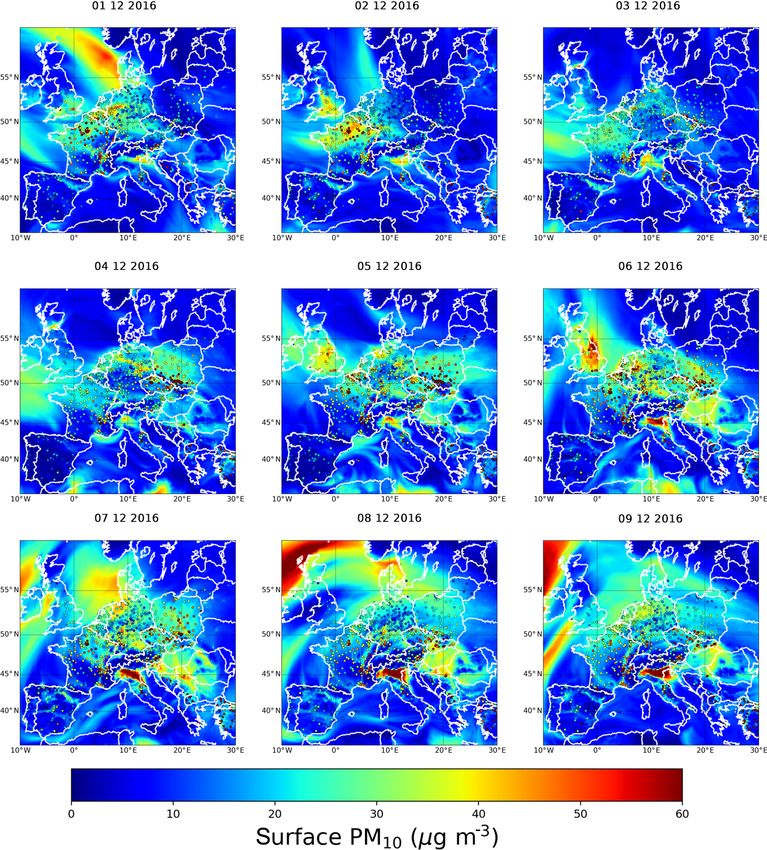
During December 2016, a PM episode of medium inten- NMB is calculated by Eq. (2):
sity (no more than 3 consecutive days beyond the WHO
N
PM10 threshold) developed across north-western Europe. As P
(Mi − Ri )
a consequence of a high pressure system over central Eu- i=1
NMB = × 100 %. (2)
rope pollutant concentrations were built up over western N
P
Europe (see http://policy.atmosphere.copernicus.eu/reports/ Ri
i=1
CAMSReportDec2016-episode.pdf, last access: 24 January
2020). RMSE is calculated by Eq. (3) and expressed in micrograms
From 1 to 2 December, high concentrations were measured per cubic metre as follows:
and predicted over Paris (Figs. 1 and 2). In Fig. 2, we can v
u N
also see from 3 to 8 December that levels of PM10 were el-
u (Mi − Ri )2
uP
evated in western Europe. Especially on 6 and 7 December, t i=1
concentrations at some measurement stations in France, Bel- RMSE = , (3)
N
gium, the Netherlands, Germany, and Poland exceeded the
daily limit value of 50 µg m−3 (e.g Fig. S2 – see Sect. 3.2 for and FGE is calculated by Eq. (4) and is dimensionless,
more details about the observations).
N
During the following days relatively stable conditions with 2 X |Mi − Ri |
FGE = . (4)
slow southerly winds characterized the episode until fronts N i=1 |Mi + Ri |
moved in western Europe on 9 December. Large concen-
trations (> 60 µg m−3 ) were also predicted between 6 and 3.2 Comparison with observations
9 December over the Po Valley and over UK on 6 Decem-
ber (Figs. 2 and S2). 3.2.1 Methodology
3.1 Statistical metrics used In order to evaluate the reliability of the predic-
tions over each city, the modelled hourly PM10 con-
To properly estimate the quality of these forecasts, five statis- centrations have been compared with the AirBase
tical parameters have been used, including the Pearson cor- data (see https://www.eea.europa.eu/data-and-maps/
relation (r), the mean bias (MB), the normalized mean bias data/airbase-the-european-air-quality-database-8#
(NMB), the root-mean-square error (RMSE), and the frac- tab-data-by-country, last access: 27 March 2020). The
tional gross error (FGE). The ideal score of these parameters traffic stations were not included in the comparison since
is 0, except for the correlation, which is 1. a regional model with a somewhat-coarse resolution will
The MB provides information about the absolute bias of not be able to calculate very large concentrations (e.g.
the model, with negative values indicating underestimation hourly concentration higher than 200 µg m−3 ), which may
and positive values indicating overestimation by the model. be measured by these stations. Indeed, the concentrations
The NMB represents the model bias relative to the reference. calculated by a regional model over cities are mostly
The RMSE considers error compensation due to opposite representative of the urban background. By knowing this
sign differences and encapsulates the average error produced point, we can state that a comparison with the observations
by the model. The FGE is a measure of model error, ranging presenting for example a correlation coefficient equal to 0.5
between 0 and 2, and behaves symmetrically with respect or NMB lower than 15 % is a reasonable result (r ≥ 0.7
to under- and overestimation, without over emphasizing out- and NMB ≤ 10 % are good results). The observations have
liers. also been categorized into two sets of data by differentiating
We have used M and R as notation to refer, respectively, to between the rural stations and the urban stations (as shown
model and the reference data (e.g. observations), and N is the in Fig. S2). This follows the procedure done in the yearly
size of the reference data set (e.g. number of observations). evaluation of the EMEP model over Europe (e.g. EMEP
Status Report, 2018). Due to the relatively coarse definition
of a city, it appears that stations classified as rural may be
present in our city domain.
This was noticed for the smaller definition of the city
edges, i.e. one grid cell there were no rural stations within the
www.geosci-model-dev.net/13/1787/2020/ Geosci. Model Dev., 13, 1787–1807, 20201794 M. Pommier et al.: Prediction of source contributions to PM10 concentrations in European cities
Figure 2. Daily surface PM10 concentration, in micrograms per cubic metre, over Europe predicted by the EMEP model from 1 to 9 Decem-
ber 2016. The coloured dots correspond to the daily mean of AirBase stations (rural and urban stations).
city domain. Obviously, by increasing the size of the city do- the urban concentrations. For such a comparison, the model
main, to nine grid cells or by using the GADM definition, the concentrations are also averaged over the city domain.
number of rural stations present within the city domain in-
creases. Indeed, all of the hourly measurements are averaged
within the city boundary, by separating the urban and the ru- 3.2.2 Results
ral stations. A comparison with these two types of stations
can highlight a difference between the urban background and Figures 3 and 4 show the comparison between the hourly
averaged observations within the city edges defined by the
Geosci. Model Dev., 13, 1787–1807, 2020 www.geosci-model-dev.net/13/1787/2020/M. Pommier et al.: Prediction of source contributions to PM10 concentrations in European cities 1795
closer to the target date. The available observations and thus
the stations may also differ from day to day (e.g. Fig. S2a).
Figures 3 and 4 also show that despite many differences, the
models have very similar performances in comparison with
the urban stations.
In Fig. 3, it is also clear that the EMEP model has difficul-
ties reproducing the highest concentrations measured by the
urban stations, which are probably smoothed by the model
over the large grid cells, as are the ones defining the cities.
The underestimation of the largest urban concentrations is
highlighted by the comparison with the rural stations. This
also shows that over the area defining the cities there is a
large variability in the measured PM10 concentrations and
that few stations are not necessarily representative of the
model grids. It also shows with such a resolution, the model
represents urban background concentrations.
Figure 3. Scatterplots between the hourly PM10 concentrations, in
micrograms per cubic metre, over all of the studied cities using the Only five cities have measurements defined as rural sta-
nine grid cells definition, predicted by the EMEP model on 6 De- tions by using the nine grids definition (i.e. Amsterdam,
cember 2016 and the observations of the urban sites (blue dot) and Berlin, Luxembourg, Rotterdam, and Vienna) while there
rural sites (red square). For this case, there are 19 cities which have are up to 19 cities with urban stations. By comparing only
urban stations in their domain and five cities which have rural sta- the five cities having urban and rural stations, the agreement
tions in their domain. The observations are collocated in time with between EMEP and the urban stations is largely improved
the EMEP predictions and then averaged within the city edge to as shown in Fig. S3. We also notice that the difference in
match the studied grid. The four panels correspond to the different concentrations predicted by the EMEP model between both
predictions from 3 d before the 6 December to the actual day, i.e. types of stations is also reduced. This shows that for these
6 December. The correlation coefficient (r), the mean bias (MB), the
five cities, the predicted PM10 concentrations on 6 Decem-
normalized mean bias (NMB), the root-mean-square error (RMSE),
ber are higher than over the other cities.
and the fractional gross error (FGE) are provided on each panel. The
blue and the red lines represent the linear fits. LOTOS-EUROS is less correlated with the concentrations
measured by the rural stations than EMEP (Fig. 4). However,
like EMEP, LOTOS-EUROS also presents a lower bias for
these rural stations in comparison with the urban stations.
This is predictable since with such a resolution, the model
calculates mainly the urban background concentrations. By
comparing the five cities having urban and rural stations, as
done with EMEP, only the bias and the FGE between the pre-
dictions and the urban measurements are improved (Fig. S4).
It is also worth noting that the concentrations predicted by
LOTOS-EUROS over these five cities are lower than the ones
calculated by the EMEP model (in Fig. S3).
By using the GADM definition, the number of cities hav-
ing rural stations decreases to two, while the number of cities
with the urban stations remains identical.
In general, both models present similar performances rela-
tive to the observations especially for the NMB, RMSE, and
FGE as presented in Figs. S5 and S6. These figures show an
Figure 4. As Fig. 3 for LOTOS-EUROS. overview of the statistical parameters for all 4 d forecasts, i.e.
the dates from 1 to 12 December 2016 with a starting date
from 1 to 9 December, for all of the cities defined by nine
nine grid cells definition and the predictions from EMEP and grid cells, in comparison with the concentrations measured
from LOTOS-EUROS, respectively. at the urban and the rural stations, respectively.
Figures 3 and 4 show that for the urban stations, the dif- As already shown by Figs. 3 and 4, LOTOS-EUROS
ferent predictions from the same model, for the same date, shows slightly better correlation coefficients for the urban
are consistent since the values for the statistical parameters stations than EMEP (Fig. S5; on average RLOTOS-EUROS =
are relatively constant. It is noticed, however, that the bias 0.31 and REMEP = 0.25, with a maximum of 0.58 for
is slightly reduced when the starting date of the forecast is LOTOS-EUROS and 0.5 for EMEP) and EMEP presents bet-
www.geosci-model-dev.net/13/1787/2020/ Geosci. Model Dev., 13, 1787–1807, 20201796 M. Pommier et al.: Prediction of source contributions to PM10 concentrations in European cities
ter correlations with the few rural stations (Fig. S6; on aver- (which is not diagnosed as mentioned in Sect. 2). More-
age RLOTOS-EUROS = 0.23 and REMEP = 0.35, with a maxi- over, it confirms the larger PM10 concentrations predicted by
mum of 0.58 for LOTOS-EUROS and 0.72 for EMEP). How- EMEP than by LOTOS-EUROS for the five cities plotted in
ever, the limited number of cities having rural stations ex- Figs. S3 and S4. It is also worth noting that LOTOS-EUROS
plain the larger variability in the correlations compared to the predicts more sea salt and dust for almost all of the cities
correlations found with the urban stations. Similar results are during the studied period (Fig. S8), which is representative
found by using the GADM definition (not shown), while by of the overall feature over the regional domain (not shown).
using only one grid to define the city edges, the correlation Actually, it was noticed that for the predicted PM10 with the
coefficients with the urban stations are larger (up to 0.8), with larger positive NMB (EMEP predicting larger PM10 concen-
an increase in the bias and a decrease in the RMSE (Fig. S7). trations), EMEP has more SIA and ”other” than LOTOS-
On average, both models have a FGE equal to 0.5 over the EUROS (Fig. S9a), while the PM10 from LOTOS-EUROS
cities defined by nine grid cells with the urban stations and is dominated by natural components when a larger negative
0.4 with the rural stations. For the RMSE, it is 33 µg m−3 NMB is predicted (Fig. S9b).
with the urban stations and 11 µg m−3 with the rural stations.
While both models underestimate the PM10 concentrations
by 36 % on average by using the urban sites, EMEP overes- 4 Methodology of the source contribution calculation
timates by 6 % with the rural stations, and LOTOS-EUROS
underestimates this by 6 %. 4.1 The EMEP model
Performances of both models are improved with daily
means, especially with better correlation coefficients (not 4.1.1 Emission reductions
shown). For example, with the cities defined by nine grid
The SC calculation follows the methodology used in each
cells, the correlation coefficients reach 0.8 with the urban sta-
EMEP annual report to quantify the annual country-to-
tions for EMEP and LOTOS-EUROS and 0.98 with the rural
country source–receptor relationships (e.g. EMEP Status Re-
stations for EMEP. However, a lot of negative correlation co-
port, 2018). The experiment is based on a reference run,
efficients between LOTOS-EUROS and the rural stations are
where all of the anthropogenic emissions are included. The
noticed. The correlation coefficient with the rural stations re-
other runs are the perturbation runs. These runs correspond
mains difficult to interpret, related to the limited number of
to the simulations where the emissions from every consid-
stations available. Thus, EMEP presents a mean correlation
ered country are reduced by 15 %. As explained in Wind et
coefficient equal to 0.4 for the urban and rural stations, and
al. (2004), a reduction of 15 % is sufficient to give a clear sig-
LOTOS-EUROS has a mean correlation of 0.5 with the urban
nal in the pollution changes. It also causes a negligible effect
stations and only 0.06 with the rural stations. Better scores
from nonlinearity in the chemistry even if in this work it has
with the FGE and the RMSE are also noticed in comparison
been estimated.
to the hourly evaluation (not shown). Both models present,
The perturbation runs are done for anthropogenic emis-
with the nine grid cells definition, a mean FGE of 0.5 with
sions of CO, SOx , NOx , NH3 , non-methane volatile organic
the urban stations and 0.3 for the rural stations and a mean
compounds (NMVOCs), and PPM (primary particulate mat-
RMSE of 21 µg m−3 with the urban stations and 10 µg m−3
ter). For computational efficiency, in the perturbation calcu-
with the rural stations.
lations, all anthropogenic emissions in the perturbation runs
have been reduced here simultaneously. This simultaneous
3.3 Intercomparison in the concentrations predicted by
reduction differs from the methodology used in each EMEP
both models
annual report where the emissions are reduced individually.
There are in total 31 runs for each date with reduced an-
The second analysis has been focused on the agreement be-
thropogenic emissions. Each run corresponds to the perturba-
tween both models. During the episode, all 4 d forecasts
tions for one of the 28 countries related to the 28 EU capitals,
present a high correlation between the PM10 predicted by
plus Iceland, Norway and Switzerland, giving the contribu-
the EMEP model and LOTOS-EUROS as shown in Fig. 5a.
tion for each country.
These correlations vary from day to day and city by city
To calculate the concentration of the pollutant integrated
but remain large for the different simulated periods (me-
over the studied area, i.e. a selected city, coming from a
dian = 0.7).
source, we follow the Eq. (5):
There is no clear geographical pattern in terms of perfor-
mance between the two models, even if the central Euro- Creference − Cperturbation
pean cities (e.g. Budapest, Vienna, and Warsaw) presented Csource = , (5)
x
the larger differences (Fig. 5b). These differences may be ex-
plained by not only by slightly lower secondary inorganic where x is the reduction in percent (i.e. 0.15), Creference is the
aerosols (SIA = NO− + 2
3 + NH4 + SO4 −) in LOTOS-EUROS concentration of the pollutant integrated over the studied area
for these cities but also the lack of water in LOTOS-EUROS from the reference run, and Cperturbation is the concentration
Geosci. Model Dev., 13, 1787–1807, 2020 www.geosci-model-dev.net/13/1787/2020/M. Pommier et al.: Prediction of source contributions to PM10 concentrations in European cities 1797
Figure 5. (a) Correlation coefficient and (b) bias in the predicted PM10 concentrations between the EMEP model and LOTOS-EUROS
over all of the studied cities using the nine grid cells definition for each 4 d forecast (1–4, 2–5, 3–6, 4–7, 5–8, 6–9, 7–10, 8–11, and 9–
12 December 2016).
of the pollutant integrated over the studied area from the per- and the sum from the various sources may lead to negative
turbation run. Thus, by differentiating over the studied area, or positive concentrations. This is a result of the perturbation
the concentration from the perturbed run with the concentra- used, which is assumed to be linear for a 100 % perturbation.
tion provided by the reference run, we have an estimation of The 15 % emission reduction has been used for many years
the influence of the source (i.e. country). By scaling with the for the annual country-to-country source–receptor relation-
reduction used (parameter x), it gives the estimated concen- ships calculations (e.g. EMEP Status Report, 2018). Clap-
tration related to the source. pier et al. (2017a) have already shown the robustness of the
methodology at the country scale on yearly averages and for
4.1.2 Issue concerning the chemical nonlinearity the highest daily concentrations. However, this emission re-
duction was not used for smaller areas. Thus this 15 % emis-
The reason why emissions should not be perturbed by 100 % sion reduction for the study over a city and on hourly basis
in the model simulations is to stay within the linear regime of has been tested, in order to assess the robustness of the cal-
involved chemistry. Even limited, such a methodology may culations. The values 5 % and 50 % were the other selected
still introduce a nonlinearity in the chemistry. The total PM10 emission reductions. In total, 847 4 d runs have been per-
over the receptor should be identical theoretically to the sum formed in this work (nine reference runs and nine dates ×
of the PM10 originated from the different sources. This is not 31 countries × 3 perturbations runs).
always the case, and the difference between the total PM10
www.geosci-model-dev.net/13/1787/2020/ Geosci. Model Dev., 13, 1787–1807, 20201798 M. Pommier et al.: Prediction of source contributions to PM10 concentrations in European cities
Furthermore, by reducing the emissions simultaneously or tion from the domestic country to the city (for example from
separately may lead to a different result in the concentrations, France to Paris). The 30 European countries corresponds to
but as mentioned previously, this effect is not addressed in the other 30 European countries used in the study. Others
this work for computational reasons. contains mainly natural sources, the other European coun-
tries included in the regional domain (and not included in
4.2 LOTOS-EUROS our SC calculations, e.g. Turkey), and the boundary condi-
tions. This figure gives a graphical illustration of the compo-
A labelling technique has been developed within each sition of the different contributions and presents the effect of
LOTOS-EUROS simulation (Kranenburg et al., 2013). An the nonlinearity. Indeed, the positive concentrations show the
important advantage of the labelling technique is the reduc- overall composition for each contribution, while the chemi-
tion in computation costs and analysis work associated with cal reason of the nonlinearity is highlighted by the negative
the calculations. The source apportionment technique has contribution to the predicted PM10 concentrations.
been previously used to investigate the origin of PM (Hen- The main contributors to the Domestic PM10 are POM
driks et al., 2013, 2016), NO2 (Schaap et al., 2013), and ni- (∼ 20 %) and rest PPM (∼ 30 %) (which corresponds to the
trogen deposition (Schaap et al., 2018). remainder of coarse and fine PPM), as noticed for the positive
Besides the concentrations of all species, the contributions concentrations (Fig. 6a). Actually, the variation in the mean
of a number of sources to all components are calculated. concentrations is mainly influenced by the variation in these
The labelling routine is only implemented for primary, in- primary components. NO− 3 is also an important component
ert aerosol tracers and chemically active tracers containing of the Domestic PM10 . The value of the mean concentration
a C, N (reduced and oxidized), or S atom, as these are con- depends on the city definition ,and so on the average of the
served and traceable. This technique is therefore not suitable concentrations over different size of city. The mean PM10
to investigate the origin of e.g. O3 and H2 O2 , as they do not concentration over a smaller area is larger, showing that with
contain a traceable atom. The source apportionment module a smaller grid, the PM10 is less diffused over the integrated
for LOTOS-EUROS provides a source attribution valid for area. The 30 European countries PM10 is mainly influenced
current atmospheric conditions as all chemical conversions by NO− 3 (by 38 %) (Fig. 6b).
occur under the same oxidant levels. For details and valida- Overall, 45 % of the contributions to the PM10 calculated
tion of this source apportionment module we refer to Kra- over the selected cities for this episode are Domestic and
nenburg et al. (2013). essentially due to primary components. 35 % are from the
To avoid violating the memory size and to avoid excessive 30 European countries, essentially NO− 3 , and 25 % are from
computation times it was chosen to trace the 28 EU countries, Others, mainly composed of natural sources (representing
supplemented by Norway and Switzerland. For convenience, 50 % of Others). Obviously, this feature is an overview of
a number of small countries were combined with a neigh- all selected cities for all of the studied dates and it can vary
bouring country. For example, Switzerland and Liechtenstein from city to city and from date to date.
and Luxembourg and Belgium were combined. In addition, By comparing the PM10 concentrations calculated over the
all sea areas were combined into one source area. To be mass same city edges but by using different percentages in the per-
consistent, all non-specified regions, natural emissions, and turbation runs, we have calculated the impact of the non-
the combined impact of initial conditions and boundary con- linearity for each contribution and presented this in Fig. 7.
ditions were given labels as well. This nonlinearity has been calculated for each hourly con-
centration as the standard deviation of the hourly contribu-
5 Information provided by the source contribution tion (which can be positive or negative) obtained by the three
calculations reduced emissions scenarios and weighted by the hourly total
concentration by following the Eq. (6):
5.1 In the EMEP calculations s
n
P 2
Ccontribi −Ccontrib
As presented in Fig. 1, the country contributions to the pre- i=1
n
dicted PM10 concentrations in the cities is provided in our NONLINContrib = × 100 %, (6)
Ctot
products.
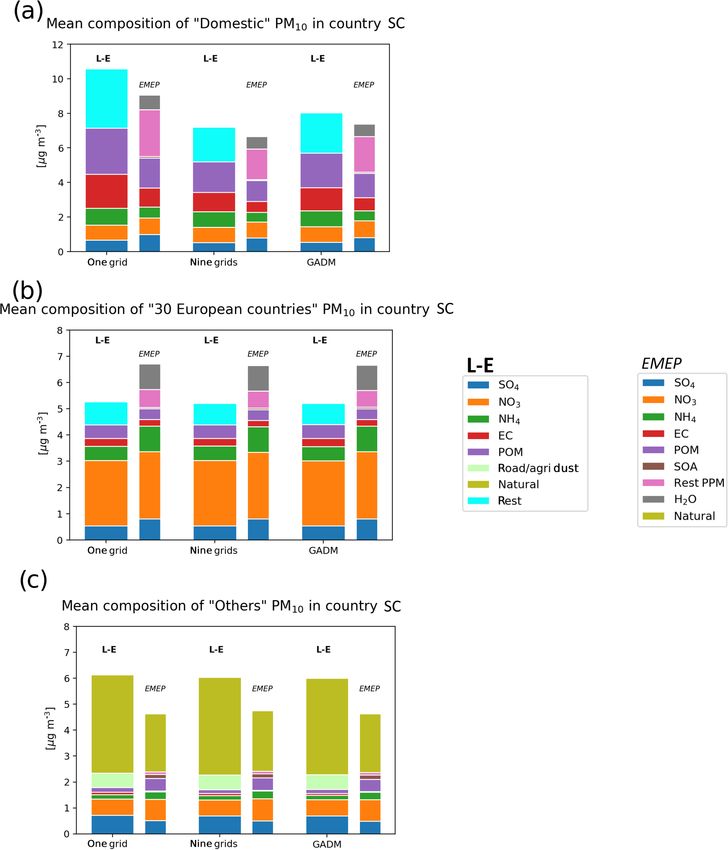
Figure 6 presents the mean composition for the “Domes- where n corresponds to the number of perturbations used
tic”, “30 European” countries, and “Others” PM10 contribu- (n = 3), Ccontrib is the hourly PM10 concentration for a spe-
tions for all cities, for all 4 d predictions, and split into neg- cific contribution (Domestic, 30 European countries, or Oth-
ative and positive concentrations. This figure is a result of ers), and Ctot is the hourly PM10 concentration. This mean
the perturbation runs by separating the positive and the neg- nonlinearity due to the Domestic contribution represents a
ative concentrations obtained in the calculations. The con- maximum of 0.9 % of the total PM10 . This nonlinearity from
centrations have also been gathered by their calculated ori- the 30 European countries contribution counts for 0.7 % of
gin. The Domestic contribution corresponds to the contribu- the total PM10 and 1.5 % from Others. Actually, the non-
Geosci. Model Dev., 13, 1787–1807, 2020 www.geosci-model-dev.net/13/1787/2020/M. Pommier et al.: Prediction of source contributions to PM10 concentrations in European cities 1799
Figure 6. Mean composition of (a) Domestic, (b) 30 European countries, and (c) Others PM10 , split into a negative concentration (left panel)
and a positive concentration (right panel), calculated by the EMEP country SC over the 34 European cities and for each 4 d forecast. The
PM10 composition is highlighted with the colour code. The results for the three city definitions (one grid, nine grids, and GADM) and for
the percentage of reduction used in the perturbation EMEP runs (5 %, 15 %, and 50 %) are shown. The Domestic contribution corresponds
to the contribution from the domestic country to the city (e.g. from France to Paris). The label 30 European countries corresponds to the
other 30 European countries used in the study. Others contains natural sources, the other countries included in the regional domain, boundary
conditions, ship traffic, biogenic sources, aircraft emissions, and lightning. The red dot represents the mean PM10 concentration.
linearity from the Others depends on the nonlinearity from not the one related to the reduction in each emission precur-
the two other contributions. The mean nonlinearity is not ho- sor has been estimated in this study as mentioned in Sect. 4.1.
mogenously distributed over all cities as shown in Fig. S10 Negligible negative contributions have been calculated
and may vary from date to date (not shown). It has remained for the Domestic and 30 European countries contributions
limited even if some hourly contributions show higher non- (Fig. 6a and b), and small negative contributions are pre-
linearity. At the maximum, 3 % of the calculated hourly con- dicted in Others (Fig. 6c). These negative PM10 are a result
tributions for all 4 d forecasts over the selected cities have of negative values in NO− +
3 , NH4 , and H2 O, which are a con-
a nonlinearity higher than 5 % (not shown). This shows that sequence of gas–aerosol partitioning of the species. Indeed,
due to the methodology used in the EMEP model, based on a NH3 reacts with nitric acid (HNO3 ) to form ammonium ni-
reduced emission scenario, the nonlinearity in the chemistry trate (NH4 NO3 ). This is an equilibrium reaction and thus the
has a limited impact on the SC calculation. This nonlinearity transition from solid to gaseous phase depends on relative
is slightly reduced by using the larger domains to define the humidity (e.g. Fagerli and Ass, 2008; Pakkanen, 1996). This
cities (e.g. nine grids) (Fig. 7). This also shows that the re- shows that, for example, a reduction in NOx over a country,
sponses to perturbation runs are robust, even if only the non- which impacts the selected city, does not necessarily only
linearity in the chemistry related to the perturbation used and impact the NO− 3 over this city but may also have an effect
www.geosci-model-dev.net/13/1787/2020/ Geosci. Model Dev., 13, 1787–1807, 20201800 M. Pommier et al.: Prediction of source contributions to PM10 concentrations in European cities
Averaging out over the larger grids reduces globally the
nonlinearity. The 15 % emission reduction also reduces the
negative nonlinearity in the Domestic concentrations (e.g.
H2 O for the nine-grid and GADM runs).
5.2 In the LOTOS-EUROS calculations
As presented with the EMEP predictions, Figure 8 presents
the mean composition for the Domestic, 30 European coun-
tries, and Others PM10 contributions for all cities, for all 4 d
predictions provided by LOTOS-EUROS. The definition of
Others is slightly different from the EMEP one since, for ex-
ample, the dust from agriculture and traffic is included (see
Sect. 2). For an easier comparison, the result for the EMEP
model using the 15 % emission reduction has also been plot-
ted with thinner charts, even if, as just mentioned, the defini-
tion of Others slightly differs between both models.
First of all, during the episode, LOTOS-EUROS confirms
the general trend calculated by the EMEP model, i.e. the
dominant contribution to the surface PM10 is Domestic, rang-
ing between 40 % and 48 % of the predicted PM10 over all
selected cities and for all of the studied dates. However,
LOTOS-EUROS always presents more Domestic PM10 than
the EMEP model. LOTOS-EUROS also predicted slightly
more influence from Others than the 30 European countries,
with ratios close to 25 %–30 % each. As a reminder, the
EMEP model predicted a slightly larger influence from the
30 European countries (35 %) than from Others (25 %).
As with the EMEP model, the mean PM10 concentration
over the smaller city definition is larger, and the Domes-
tic PM10 is largely driven by POM. In the list of LOTOS-
EUROS PM10 components there is one named “Rest”. Rest
corresponds to the difference between the total PM10 and the
sum of all of the components, and Fig. 8 shows that it is also a
large component of this Domestic PM10 . POM and Rest each
represent between 25 % and 30 % of the Domestic PM10 .
The large influence of NO− 3 (48 %) on the 30 European
countries PM10 is also calculated by LOTOS-EUROS, as
Figure 7. The black horizontal bars show the mean nonlinearity well as the large contribution of the natural components
calculated for each contribution presented in Fig. 6 and for the (60 %) in Others. It is noteworthy to see that, even being
three city definitions. The nonlinearity is calculated for each hourly small, the dust emitted by the road traffic and the agriculture
concentration as the standard deviation of the hourly contribution is not negligible in Others PM10 (∼ 10 %).
weighted by the hourly total concentration.
6 Comparison between both country source
on NH3 chemistry over a second region. This second region
contribution calculations
may also have itself an impact on the selected city. This com-
bination of NOx and NH3 chemistry from different regions
Section 3 has highlighted the similar performance of both
may lead at the end to these negative concentrations.
models in the prediction of the PM10 concentrations over the
The impacts of the percentage used in the perturbation
European cities with observations. It has also been shown in
runs and the size of the city edges have no significant im-
Sect. 3 that both models are representative for a large area,
pact on the amount of negative Others PM10 concentrations.
and the predictions can underestimate the concentrations and
The impact of both parameters is more visible on the Domes-
the contributions for the larger concentrations measured by a
tic and 30 European countries concentrations but it remains
specific station. Section 5 has shown similar results in terms
very small.
of composition of these PM10 . It is also noteworthy to see in
Geosci. Model Dev., 13, 1787–1807, 2020 www.geosci-model-dev.net/13/1787/2020/You can also read