Comparing hundreds of machine learning classifiers and discrete choice models in predicting travel behavior: an empirical benchmark
←
→
Page content transcription
If your browser does not render page correctly, please read the page content below
Comparing hundreds of machine learning classifiers and
                                        discrete choice models in predicting travel behavior: an
                                                         empirical benchmark
                                                    Shenhao Wang1,4,* , Baichuan Mo3 , Stephane Hess2 , Jinhua Zhao1
arXiv:2102.01130v1 [cs.LG] 1 Feb 2021

                                               1 - Department of Urban Studies and Planning, Massachusetts Institute of Technology
                                                 2 - Choice Modeling Centre & Institute for Transport Studies, University of Leeds
                                           3 - Department of Civil and Environment Engineering, Massachusetts Institute of Technology
                                                              4 - Media Lab, Massachusetts Institute of Technology

                                                                                    January 2021

                                                                                     Abstract
                                           A growing number of researchers have compared machine learning (ML) classifiers and discrete
                                           choice models (DCMs) in predicting travel behavior, but the generalizability of the findings is
                                           often limited by the specifics of data, contexts, and authors’ expertise. This study seeks to
                                           provide a definitive and generalizable empirical benchmark by comparing hundreds of ML and
                                           DCM classifiers in a highly structured manner. The experiments evaluate both prediction accu-
                                           racy and computational cost by spanning four hyper-dimensions, including 105 ML and DCM
                                           classifiers from 12 model families, 3 datasets, 3 sample sizes, and 3 outputs. This experimental
                                           design leads to an immense number of 6,970 experiments, which are further corroborated with
                                           a meta dataset of 136 experiment points from 35 previous studies. This study is hitherto the
                                           most comprehensive and an almost exhaustive comparison of the classifiers for travel behavioral
                                           prediction.
                                               We found that the ensemble methods, including boosting, bagging, and random forests,
                                           and deep neural networks, achieve the highest predictive performance, but at a relatively high
                                           computational cost. Random forests are the most computationally efficient, thus balancing
                                           between prediction and computation. While discrete choice models can offer accuracy with
                                           only 3-4 percentage points lower than the top ML classifiers, they have much longer computa-
                                           tional time and become computationally impossible with large sample size, high input dimen-
                                           sions, or simulation-based estimation. The relative ranking of the ML and DCM classifiers is
                                           highly stable, while the absolute values of the prediction accuracy and computational time have
                                           large variations. Prediction accuracy varies significantly with datasets, and larger sample size
                                           leads to moderately higher prediction but significantly longer computational time. Overall, this
                                           paper suggests to use deep neural networks, model ensembles, and random forests as baseline
                                           models for future travel behavior prediction. It also suggests a synergetic perspective between
                                           the ML classifiers and DCMs, and further research into versatile neural network architectures.
                                           For choice modeling, the DCM community should switch more attention from fitting models to
                                           improving computational efficiency, so that the DCMs can be widely adopted in the big data
                                           context.
                                           Keywords: Machine learning; choice modeling; travel behavior; prediction.

                                         Corresponding author: Shenhao Wang; email: shenhao@mit.edu
1. Introduction
Travel behavior prediction is a fundamental topic in transportation research [3, 10, 4, 63, 15]. Al-
though this topic has traditionally been addressed by discrete choice models (DCMs) [67], researchers
have started to predict travel behavior by using a long list of machine learning (ML) classifiers and
comparing them to the classical DCMs [28, 72, 12]. The comparative studies are important since
they provide insights into model selection, reveal novel behavioral mechanisms different from ran-
dom utility maximization, and improve the performance of demand forecasting with the new ML
classifiers. However, the comparative studies can rarely provide a definitive and generalizable con-
clusion about the predictive power of the ML and DCM classifiers1 , since they are often limited by
the specifics of data, contexts, or authors’ expertise. For example, researchers might choose a spe-
cific ML classifier simply due to coding convenience or based on their own expertise. Or they may
find that ML classifiers outperform DCMs only because of the particularity of the datasets or the
research contexts. These two issues, i.e. model selection as well as application context, inevitably
limit the generalizability of their conclusions. Therefore, a useful empirical benchmark is still lack-
ing in the travel demand modeling community, since a critical question is unresolved: how to use
a single study to provide a generalizable empirical benchmark for the comparative performance of
the ML and DCM classifiers in predicting travel behavior?
To answer this question, we first define the concepts of hyper-dimensions, experiment point,
and experiment space. Hyper-dimensions are defined as the aspects that significantly influence
the predictive performance of a classifier, and these include the type of classifiers, datasets, sample
sizes, outputs2 , among others. An experiment point is defined as a model trained with given fixed
hyper-dimensions. For example, an experiment point can be a multinomial logit model trained with
a specific dataset of 1,000 observations to predict travel mode choices. The experiment space is
defined as the space including all the experiment points spanned by the hyper-dimensions. These
three concepts can be intuitively understood from the perspective of a meta-analysis, which draws
conclusions by integrating the results from many past studies that aim to solve the same problem
[19]. A meta-analysis can be seen as a summary of an experiment space, in which each past
study serves as an experiment point. Therefore, a single study can yield generalizable results when
it resembles the nature of a meta-analysis by incorporating critical hyper-dimensions, a typically
vast experiment space, and a comprehensive, representative, and relevant list of experiment points.
Unfortunately, none of the past studies comparing the performance of ML and DCM classifiers has
achieved this goal because they did not make these concepts explicit, let alone satisfying the criteria.
The present study seeks to provide a definitive and generalizable empirical benchmark about
the performance of the ML and DCM classifiers in predicting travel behavior by investigating a
tremendous experiment space consisting of four hyper-dimensions and 1,394 experiment points.
1
We will use the term classifiers throughout the rest of this paper. It is the common term used in ML, while in
choice modelling, the term model is more common.
2
Inputs and outputs are commonly used in the ML literature, and they are corresponding to independent variables
and dependent variables in choice modeling.
1Empirically, we seek to (1) identify the globally best model family and classifiers for travel behavior
prediction, (2) provide insights into how model performance varies across datasets, sample size, and
outputs, and (3) discuss the pros and cons of ML classifiers and DCMs in terms of both prediction
accuracy and computational time. We chose prediction accuracy as the metric to evaluate predictive
performance, since it is nearly the only metric allowing the comparison across a large number of
classifiers. We documented the computational time to evaluate the computational burden, which
is important since a theoretically feasible model can be deemed as practically impossible when
the computational time3 is extremely long. We designed a large-scale experiment spanning four
hyper-dimensions, including 105 classifiers from 12 model families as the primary hyper-dimension,
and 3 datasets, 3 sample sizes, and 3 travel behaviors as three secondary hyper-dimensions. The
hyper-dimensions are organized as follows.
• Classifiers. The primary hyper-dimension is the classifiers. The experiments examine 105
classifiers from the 12 most important model families, including (1) discrete choice models
(DCM; 3 models), (2) deep neural networks (DNN; 15 models), (3) discriminant analysis
(DA; 12 models), (4) Bayesian methods (BM; 7 models), (5) support vector machines (SVM;
9 models), (6) K nearest neighbors (KNN; 4 models), (7) decision trees (DT; 14 models),
(8) generalized linear models (GLM; 10 models), (9) Gaussian process (GP; 3 models), (10)
bagging (3 models), (11) random forests (RF; 2 models), and (12) boosting (23 models).
• Datasets. Three datasets are used, including the US national household travel survey 2017
(NHTS2017), the London travel demand survey 2015 (LTDS2015), and a stated preference
survey collected in Singapore in 2017 (SGP2017). The three datasets cover two important
data collection procedures - revealed and stated preference surveys - and three geographical
locations in America, Europe, and Asia.
• Sample sizes. The sample size includes 1,000, 10,000, and 100,000 observations, which can
represent the main scales of the sample sizes in the travel behavior research.
• Outputs. The outputs include three travel behaviors: travel mode choice, car ownership, and
trip purposes. Owing to data limitation, car ownership and trip purposes are only available
in the NHTS2017 dataset.
In this experiment, a single classifier trained on a dataset, a sample size, and a targeting output
is an experiment point; for example, an experiment point can refer to a multinomial logit model
trained on NHTS2017 with 1,000 observations to predict travel mode choice. All the experiment
points together constitute our experiment space. Only with this highly structured experiment design
and a massive number of experiments can it be possible to identify a generalizable result for the
comparative performance of ML and DCM classifiers in predicting travel behavior.
We defined the concepts of hyper-dimensions, experiment points, and experiment space so that
we can jointly analyze the large-scale experiments and a meta dataset, which is a literature review
summarizing 136 experiment points from 35 previous studies. The joint analysis is possible since
3
In choice modelling, the term estimation time is used more commonly.
2the modeling results from these previous studies are also valid experiment points with insightful
hyper-dimension information. The meta dataset is organized by the four hyper-dimensions and
used to inform our experiment design and corroborate with our empirical results. The meta dataset
and the empirical experiments complement each other: the empirical experiments prevail in the
completeness of classifiers, while the meta dataset is particularly strong in the richness of contexts
and data types. A joint analysis can further improve the generalizability and the validity of our
findings.
The remainder of this paper is organised as follows. The next section introduces the meta dataset
of previous studies, serving as our literature review. Section 3 discusses the experiment design for
the four hyper-dimensions, with a specific focus on the list of classifiers. Section 4 summarizes other
aspects of the experiment design, such as data processing and computational process. Section 5
presents the empirical results of the large-scale experiments. Section 6 compares the results from
our empirical experiments to the meta dataset of the previous studies. Section 7 summarizes the
findings about model performance, computational time, and the effects of the hyper-dimensions.
Section 8 presents discussions and future research possibilities. Appendix I includes a table of
acronyms and terminology to translate the terminology between ML classifiers and DCMs.
2. Literature review: a meta dataset
The authors collected a meta dataset of 35 previous studies and 136 experiment points, as shown
in Table 1. This meta dataset is organized by the four hyper-dimensions, with the first column
indexing the studies, the second column presenting the author-year information, the third column
the three outputs, the fourth column the sample size, the fifth column the number of experiment
points and compared models, and the last column the best model. Each row compiles several
experiment points trained on the same dataset, so that the models on every row are comparable.
Four studies, indexed as 12, 22, 34, and 35, used more than one dataset, so they are divided into
more than one row [82, 60, 74, 73]. Although this meta dataset is not exhaustive, the structure in
Table 1 can inform our experiment design. This meta dataset is also used to validate our empirical
findings, which will be discussed in Section 6.
Study Author (Year) Tasks Sample Number of Experiment Points Best
Index Size - Compared Models Model
1 Nijkamp et al. (1996) [50] MC 1, 396 2 - DNN, MNL DNN
2 Rao et al. (1998) [56] MC 4, 335 2 - DNN, MNL DNN
3 Hensher and Ton (2000) [31] MC 1, 500 2 - DNN, NL DNN/NL
4 Sayed and Razavi (2000) [58] MC 7, 500 2 - MNL, DNN DNN
5 Cantarella et al. (2002) [9] MC 2, 808 3 - DNN, MNL, NL DNN
6 Mohammadian et al. (2002) [46] CO 597 2 - DNN, NL DNN
7 Doherty and Mohammadian TP 5, 583 2 - DNN, GLM DNN
(2003) [16]
8 Xie et al. (2003) [80] MC 4, 747 3 - DT, DNN, MNL DNN
9 Cantarella et al. (2005) [10] MC 1, 067 2 - DNN, MNL DNN
310 Celikoglu (2006) [11] MC 381 4 - DNN, MNL DNN
11 Tortum et al. [66] MC 441 3 - MNL, GLM, DNN DNN
12 Zhang and Xie (2008) [82] MC 1, 000 3 - MNL, DNN, SVM SVM
12 Zhang and Xie (2008) [82] MC 2, 000 3 - MNL, DNN, SVM SVM
13 Biagioni et al. (2008) [5] MC 19, 118 4 - MNL, BM, BOOSTING, DT BOOSTING
14 Xian and Jian (2011) [79] MC 4, 725 3 - SVM, NL, DNN SVM
15 Allahviranloo and Recker (2013) TP 3, 671 2 - SVM, MNL SVM
[2]
16 Omrani et al. (2013) [52] MC 3, 673 6 - DNN, SVM, KNN, MNL, DT, DNN
BM
17 Ermagun et al. (2015) [18] MC 4, 700 2 - NL, RF RF
18 Jahangiri et al. (2015) [37] MC N.A. 6 - KNN, SVM, DT, BAGGING, RF
RF, MNL
19 Tang et al. (2015) [65] MC 72, 536 2 - DT, MNL DT
20 Omrani (2015) [51] MC 9, 500 4 - DNN, RBFNN, MNL, SVM DNN
21 Shafique et al. (2015) [60] MC 1, 968 4 - SVM, BOOSTING, DT, RF RF
21 Shafique et al. (2015) [60] MC 1, 488 4 - SVM, BOOSTING, DT, RF RF
21 Shafique et al. (2015) [60] MC 2, 754 4 - SVM, BOOSTING, DT, RF RF
22 Shukla et al. (2015) [62] MC 100, 000 2 - DNN, DT DNN
23 Sekhar and Madhu (2016) [59] MC 4, 976 3 - RF, DT, MNL RF
24 Hagenauer and Helbich (2017) MC 230, 608 8 - MNL, DNN, NB, SVM, CTs, RF
[28] BOOSTING, BAGGING, RF
25 Paredes et al. (2017) [53] CO 15, 211 5 - MNL, BOOSTING, DT, SVM, RF
RF
26 Hillel et al. (2018) [32] MC N.A. 8 - DNN, BAGGING, BOOSTING, BOOSTING
KNN, GLM, BM, RF, SVM
27 Golshani et al. (2018) [25] MC 9, 450 2 - MNL, DNN DNN
28 Tang et al. (2018) MC 14, 000 2 -MNL, DT DT
29 Wang and Ross (2018) [72] MC 51, 910 2 - BOOSTING, MNL BOOSTING
30 Lee et al. (2018) MC 4, 764 2 - MNL, DNN DNN
31 Cheng et al. (2019) [12] MC 7, 276 4 - RF, SVM, BOOSTING, MNL RF
32 Zhou et al. (2019) [83] MC 30, 000 8 - MNL, KNN, DT, SVM, BM, BAGGING
BOOSTING, BAGGING, RF
33 Wang et al. (2020) [73] MC 8, 418 8 - MNL, NL, DNN, SVM, BM, DNN
KNN, BOOSTING, GLM
33 Wang et al. (2020) [73] MC 2, 929 8 - MNL, NL, DNN, SVM, BM, DNN
KNN, BOOSTING, GLM
34 Wang et al. (2020) [74] MC 80, 000 2 - MNL, DNN DNN
34 Wang et al. (2020) [74] MC 8, 418 2 - MNL, DNN DNN
35 Wang et al. (2020) [75] MC 8, 418 3 - NL, MNL, DNN DNN
Notes: MC - mode choice; CO - car ownership; TP - trip purposes
Table 1: A meta dataset of 35 studies and 136 experiment points
Table 1 demonstrates that the most common classifiers are MNL, NL, DNN, GLM, BM, BOOST-
ING, BAGGING, DT, RF, and SVM, all of which will be incorporated into our empirical experi-
ments. However, it also presents at least four weaknesses of the previous comparisons in choosing
4the list of classifiers. First, each study incorporated only a small number of experiment points,
which refers to not only the small number of classifiers, but also the failure to illustrate the po-
tential variations in datasets and sample sizes, among many other hyper-dimensions. Second, past
studies often failed to recognize the richness within each classifier. Many ML classifier categories,
such as DNN and BOOSTING, should not be seen as a single model. For example, DNNs can adopt
a variety of architectures and hyperparameters, so a single DNN with an arbitrary architecture can-
not represent the vast DNN model family. Third, many important classifiers are still missing. On
the ML side, the missing classifiers are discriminant analysis (DA) models and generalized linear
models (GLM). On the DCM side, the vast majority of the previous studies did not incorporate the
mixed logit model (MXL), which is a workhorse in practical travel demand modeling. Lastly, these
studies predominantly used predictive performance as the criterion, but failed to acknowledge the
practical challenges, such as the computational cost and the variation in coding languages. Although
predictive performance is important to reveal the underlying behavioral mechanism, computational
time can have practical implications even more important than prediction, since practitioners can
decide against using a theoretically ideal model when it requires hours or days in training. These
four weaknesses will be addressed in our large-scale experiments.
Every past study contains information on the hyper-dimensions - datasets, sample sizes, and
outputs; however, they failed to analyze the variation or acknowledge the impacts of the hyper-
dimensions on model performance. On the one hand, the meta dataset in Table 1 informs our
experiment design by illustrating the important values in the hyper-dimensions. In Table 1, the
sample size ranges from 381 to 230,608 observations4 , suggesting that the scale of 1,000, 10,000, and
100,000 should be able to represent the most important sample sizes in travel behavioral studies.
The previous studies analyzed travel mode choice, car ownership, and trip purposes, which can be
deemed as the most common travel behaviors. On the other side, these studies ignored the potential
variation in predictive performance caused by the hyper-dimensions: it is reasonable to postulate
that the predictive performance can vary significantly with the type of dataset and sample size,
among many other factors.
This meta dataset is not intended to be exhaustive. It excludes a vast number of studies
that used only one ML or DCM classifier, and many others that focused on spatio-temporal travel
behavior, such as traffic flow and accidents, with a data structure more complex than the classical
cross-sectional data [48, 54, 78]. The studies germane to this paper but outside the transportation
field are Fernandez-Delgado et al. (2014) and Kotsiantis et al. (2007) [20, 40], which similarly
used a large number of ML classifiers for comparison. Our comparison is limited to prediction and
computation, but other perspectives are also possible. For example, interpretability and robustness
are both critical for successfully deploying the ML methods in practice [43, 17, 47, 49, 26, 74, 73].
However, these topics are beyond the scope of the present paper and are left for future work.
4
The observations are the trips, so the number of individuals and households is smaller.
53. Experimental design: hyper-dimensions
The experiment design needs to balance the feasibility of conducting a large-scale experiment and the
ideal of incorporating as many hyper-dimensions H and values of hyper-dimensions Th as possible.
This balance is a key challenge throughout the present benchmark work. Roughly speaking, the
number of experiment points T equals to:
Y
T = |Th |; h ∈ H = {f, s, n, y}, (1)
h∈H
in which f represents classifiers; s datasets; n sample sizes; y outputs; T the total number of
experiment points; and Th the cardinality of each hyper-dimension. Hence our experiments can be
treated as a grid search for the experiment space along the four hyper-dimensions. While larger
H and Th always render our results more compelling and generalizable, both values need to be
chosen in a quite parsimonious manner to make our experiments feasible, because the complexity
T is exponential in the number of hyper-dimensions |H| and polynomial in the number of values
|Th |. This study chose four hyper-dimensions (|H| = 4), 105 classifiers (|Tf | = 105), 3 datasets
(|Ts | = 3), 3 sample sizes (|Tn | = 3), and 3 outputs (|Ty | = 3). For each hyper-dimension, this
section will demonstrate how and why certain values are incorporated while others are not, based
on the meta data of the past studies (Table 1) and the principles of completeness, relevance,
and representativeness.
3.1. Hyper-dimension 1: classifiers
The authors seek to provide a complete list of classifiers, which is summarized in Table 2 including
105 classifiers from 12 model families. Instead of treating the ML classifiers as single models, we
recognize the richness by incorporating many models into each model family. For example, to recog-
nise the significant impacts of DNN architectures on model performance, the DNN family includes
16 DNNs with different architectures and from different coding languages. However, even with our
tremendous effort, it is literally impossible to exhaust all classifiers, simply because the true number
of potential classifiers is infinite. For example, with a slight variation in model architecture, the
DNN family can present a new DNN, which might yield a predictive performance drastically differ-
ent from the 16 benchmark DNN models in our list. Therefore, to make the large-scale experiments
practically feasible, the authors only choose the representative classifiers within each model family
and the most relevant ones for travel behavioral analysis. Intuitively, DCMs are the most relevant
given their long time use in the transportation field for behavioral analysis, and DNNs are the
second most important due to the rising popularity in many subdomains in transportation [38, 73,
75]. The authors incorporate MNL, NL, and MXL into the model family of DCMs, but even so, the
nest structures in NL and the coefficients’ heterogeneity in MXL can only be prespecified following
the common standards without further detailed investigations. Nonetheless, Table 2 has presented
a relatively complete, highly representative, and highly relevant list of ML and DCM classifiers for
6travel behavioral analysis. While not completely exhaustive, it is substantially more comprehensive
than the past studies.
Classifiers Model Description Language & Function
Families
1. Discrete Choice Models (3 Models)
mnl_B DCM Multinomial logit model Python Biogeme
nl_B DCM Nested logit model (see Section 3.4 for how to nest) Python Biogeme
mxl_B DCM Mixed logit model (ASC’s as random variables) Python Biogeme
2. Deep Neural Networks (15 Models)
mlp_R DNN Multi-layer perceptrons (MLP) R RSNNS mlp
avNNet_R DNN Neural network with random seeds with averaged R Caret avNNet
scores; [57]
nnet_R DNN Single layer neural network with BFGS algorithm R Caret nnet
pcaNNet_R DNN PCA pretraining before applying neural networks R Caret pcaNNet
monmlp_R DNN MLP with monotone constraints [81] R Caret monmlp
mlp_W DNN MLP with sigmoid hidden neurons and unthresh- Weka MultilayerPerceptron
olded linear output neurons
DNN_1_30_P DNN MLP with one hidden layer and 30 neurons in each Python Tensorflow
layer
DNN_3_30_P DNN MLP with three hidden layers and 30 neurons in each Python Tensorflow
layer
DNN_5_30_P DNN MLP with five hidden layer and 30 neurons in each Python Tensorflow
layer
DNN_1_100_P DNN MLP with one hidden layer and 100 neurons in each Python Tensorflow
layer
DNN_3_100_P DNN MLP with three hidden layers and 100 neurons in Python Tensorflow
each layer
DNN_5_100_P DNN MLP with five hidden layers and 100 neurons in each Python Tensorflow
layer
DNN_1_200_P DNN MLP with one hidden layer and 200 neurons in each Python Tensorflow
layer
DNN_3_200_P DNN MLP with three hidden layers and 200 neurons in Python Tensorflow
each layer
DNN_5_200_P DNN MLP with five hidden layers and 200 neurons in each Python Tensorflow
layer
3. Discriminant Analysis (12 Models)
lda_R DA Linear discriminant analysis (LDA) model R Caret lda
lda2_R DA LDA tuning the number of components to retain up R Caret lda2
to #classes - 1
lda_P DA LDA solved by singular value decomposition without Python sklearn LinearDis-
shrinkage criminantAnalysis
sda_R DA LDA with Correlation-Adjusted T (CAT) scores for R Caret sda
variable selection
lda_shrink_P DA LDA solved by least squares with automatic shrink- Python sklearn LinearDis-
age based on Ledoit-Wolf lemma used. criminantAnalysis
slda_R DA LDA developed based on left-spherically distributed R Caret ipred
linear scores
7stepLDA_R DA LDA model with forward/backward stepwise feature R Caret stepLDA
selection
pda_R DA Penalized discriminant analysis (PDA) with shrink- R mda gen.ridge
age penalty coefficients [29]
mda_R DA Mixture discriminant analysis (MDA) where the R mda
number subclass is tuned to 3 [30]
rda_R DA Regularized discriminant analysis (RDA) with regu- R klaR
larized group covariance matrices [23]
hdda_R DA High dimensional discriminant analysis (hdda) as- R HD
suming each class in a Gaussian subspace [7]
qda_P DA Quadratic discriminant analysis (qda) Python sklearn Quadrat-
icDiscriminantAnalysis
4. Bayesian Models (7 Models)
naive_bayes_R BM Naive Bayes (NB) classifier with the normal kernel R naivebayes
density (Laplace correction factor = 2 and Band-
width Adjustment = 1)
nb_R BM NB classifier with the normal kernel density (Laplace R Caret nb
correction factor = 2 and Bandwidth Adjustment =
1)
BernoulliNB_P BM NB model with Bernoulli kernel density function Python sklearn BermoulliNB
GaussianNB_P BM NB model with Gaussian kernel density function Python sklearn GaussianNB
(smoothing = 5, according to the variance portions)
MultinomialNB_P BM NB model with multinomially distributed data Python sklearn Multinomi-
(smoothing = 1 and learn class prior probabilities) alNB
BayesNet_W BM Bayes network models by hill climbing algorithm [13] Weka BayesNet
NaiveBayes_W BM NB model with Gaussian kernel density function Weka NaiveBayes
5. Support Vector Machines (9 Models)
svmLinear_R SVM Support Vector Machine (SVM) model with linear R Caret kernlab
kernel (inverse kernel width = 1)
svmRadial_R SVM Support Vector Machine (SVM) model with Gaus- R Caret kernlab
sian kernel (inverse kernel width = 1)
svmPoly_R SVM SVM with polynomial kernel R Caret kernlab
lssvmRadial_R SVM Least Squares SVM model with Gaussian kernel R Caret kernlab
LinearSVC_P SVM SVM with linear kernel and l2 penalty Python sklearn LinearSVC
SVC_linear_P SVM SVM with linear kernel (regularization parameter = Python sklearn SVC
1)
SVC_poly_P SVM SVM with polynomial kernel (regularization param- Python sklearn SVC
eter = 1)
SVC_rbf_P SVM SVM with radial basis function (rbf) kernel (regular- Python sklearn SVC
ization parameter = 1)
SVC_sig_P SVM SVM with sigmoid function kernel (regularization pa- Python sklearn SVC
rameter = 1)
6. K Nearest Neighbors (4 Models)
KNN_1_P KNN k-nearest neighbors (KNN) classifier with number of Python sklearn KNeigh-
neighbors equal to 1 borsClassifier
KNN_5_P KNN KNN classifier with number of neighbors equal to 5 Python sklearn KNeigh-
borsClassifier
8lBk_1_W KNN KNN classifier with number of neighbors equal to 1 Weka lBk
(brute force searching and Euclidean distance) [1]
lBk_5_W KNN KNN classifier with number of neighbors equal to 5 Weka lBk
(brute force searching and Euclidean distance) [1]
7. Decision Tree (14 Models)
rpart_R DT Recursive partitioning and regression trees (RPART) R rpart
model (max depth = 30)
rpart2_R DT RPART (max depth = 10) R Caret klaR
C5.0Tree_R DT C5.0 decision tree (confidence factor = 0.25) R Caret C5.0Tree
C5.0Rules_R DT Rule-based models using Quinlan’s C5.0 algorithm R Caret C5.0Rules
[55]
ctree_R DT Conditional inference trees [35] R Caret ctree
ctree2_R DT Conditional inference trees (max depth = 10) R Caret ctree2
DecisionTree_P DT Decision tree classification model with Gini impurity Python sklearn Decision-
split measure TreeClassifier
ExtraTree_P DT Tree classifier with best splits and features chosen Python sklearn Extra-
from random splits and randomly selected features TreeClassifier
[24]
DecisionStump_W DT Tree model with decision stump Weka DecisionStump
HoeffdingTree_W DT An incremental tree with inductive algorithm. [36] Weka HoeffdingTree
REPTree_W DT Tree model using information gain/variance Weka REPTree
J48_W DT Pruned C4.5 decision tree model Weka J48
Attribute Se- DT Use J48 trees to classify patterns reduced by at- Weka AttributeSelected
lected_W tribute selection (Hall, 1998)
DecisionTable_W DT Simple decision table majority classier that uses Weka DecisionTable
BestFirst as search method [39]
8. Generalized Linear Models (10 Models)
Logistic Regres- GLM Logistic regression model with l1 penalty Python sklearn LogisticRe-
sion_l1_P gression
Logistic Regres- GLM Logistic regression model with l2 penalty Python sklearn LogisticRe-
sion_l2_P gression
Logistic_W GLM Logistic regression model with a ridge estimator [42] Weka Logistic
SimpleLogistic_W GLM Linear logistic regression models fitted by using Log- Weka SimpleLogistic
itBoost [41]
Ridge_P GLM Classifier using Ridge regression Python sklearn RidgeClassi-
fier
Passive Aggres- GLM Passive-aggressive algorithms for classification with Python sklearn PassiveAg-
sive_P hinge loss [14] gressiveClassifier
SGD_Hinge_P GLM Linear classifier with hinge loss and SGD training Python sklearn SGDClassi-
fier
SGD_Squared GLM Linear classifiers of SGD training with squared hinge Python sklearn SGDClassi-
Hinge_P loss function fier
SGD_Log_P GLM Linear classifiers of SGD training with log loss func- Python sklearn SGDClassi-
tion fier
SGD_Modified GLM Linear classifiers of SGD training with modified hu- Python sklearn SGDClassi-
Huber_P ber loss function fier
9. Gaussian Process (3 Models)
9GP_Constant_P GP Gaussian Processes classification model with con- Python sklearn GaussianPro-
stant kernel cessClassifier
GP_DotProduct_PGP Gaussian Processes classification model with Dot- Python sklearn GaussianPro-
Product kernel cessClassifier
GP_Matern_P GP Gaussian Processes classification model with Matern Python sklearn GaussianPro-
kernel cessClassifier
10. Bagging (3 Models)
Bagging_SVM_P BAGGING A bagging classifier that fits base classifiers based on Python sklearn BaggingClas-
random subsets of the original dataset; SVM is the sifier
base classifier
Bagging_Tree_P BAGGING A bagging classifier with DecisionTree as the base Python sklearn BaggingClas-
classifier sifier
Voting_P BAGGING A classifier which combine machine learning classi- Python sklearn VotingClassi-
fiers and use a majority vote. We use lda_P, Lin- fier
earSVM and Logistic classifiers here.
11. Random Forests (2 Models)
RandomForest_P RF A random forest model with 10 trees in the forest Python sklearn Random-
ForestClassifier
ExtraTrees_P RF A meta estimator that fits 10 ExtraTree classifiers Python sklearn Extra-
TreeClassifier
12. Boosting (23 Models)
AdaBoost_P BOOSTING AdaBoost classifier. The DecisionTree with maxi- Python sklearn AdaBoost-
mum depth =10 is set as the base estimator. [21] Classifier
AdaBoostM1_W BOOSTING Boosting method with DecisionStump as the base Weka AdaboostM1
classifier
AdaBoostM1_R BOOSTING Boosting method with DecisionTree as the base clas- R adabag Adaboost.M1
sifier
LogitBoost_R BOOSTING Logitboost classification algorithm using decision R LogitBoost
stumps (one node decision trees) as base learners.
Gradient Boost- BOOSTING An additive model trained in a forward stage-wise Python sklearn Gradient-
ing_P fashion [22] BoostingClassifier
DNN_1_30 Ad- BOOSTING AdaBoosting method with DNN_1_30_P as the Python Tensorflow
aBoost_P base classifier
DNN_3_30 Ad- BOOSTING AdaBoosting method with DNN_3_30_P as the Python Tensorflow
aBoost_P base classifier
DNN_5_30 Ad- BOOSTING AdaBoosting method with DNN_5_30_P as the Python Tensorflow
aBoost_P base classifier
DNN_1_100 BOOSTING AdaBoosting method with DNN_1_100_P as the Python Tensorflow
AdaBoost_P base classifier
DNN_3_100 BOOSTING AdaBoosting method with DNN_3_100_P as the Python Tensorflow
AdaBoost_P base classifier
DNN_5_100 BOOSTING AdaBoosting method with DNN_5_100_P as the Python Tensorflow
AdaBoost_P base classifier
DNN_1_200 BOOSTING AdaBoosting method with DNN_1_200_P as the Python Tensorflow
AdaBoost_P base classifier
DNN_3_200 BOOSTING AdaBoosting method with DNN_3_200_P as the Python Tensorflow
AdaBoost_P base classifier
10DNN_5_200 BOOSTING AdaBoosting method with DNN_5_200_P as the Python Tensorflow
AdaBoost_P base classifier
DNN_1_30 Gra- BOOSTING Gradient boosting method with DNN_1_30_P as Python Tensorflow
dientBoost_P the base classifier
DNN_3_30 Gra- BOOSTING Gradient boosting method with DNN_3_30_P as Python Tensorflow
dientBoost_P the base classifier
DNN_5_30 Gra- BOOSTING Gradient boosting method with DNN_5_30_P as Python Tensorflow
dientBoost_P the base classifier
DNN_1_100 BOOSTING Gradient boosting method with DNN_1_100_P as Python Tensorflow
Gradient- the base classifier
Boost_P
DNN_3_100 BOOSTING Gradient boosting method with DNN_3_100_P as Python Tensorflow
Gradient- the base classifier
Boost_P
DNN_5_100 BOOSTING Gradient boosting method with DNN_5_100_P as Python Tensorflow
Gradient- the base classifier
Boost_P
DNN_1_200 BOOSTING Gradient boosting method with DNN_1_200_P as Python Tensorflow
Gradient- the base classifier
Boost_P
DNN_3_200 BOOSTING Gradient boosting method with DNN_3_200_P as Python Tensorflow
Gradient- the base classifier
Boost_P
DNN_5_200 BOOSTING Gradient boosting method with DNN_5_200_P as Python Tensorflow
Gradient- the base classifier
Boost_P
Table 2: List of 105 ML classifiers from 12 model families
The list of classifiers is designed to address the weaknesses in past studies. For example, we
acknowledge the diversity of the classifiers by introducing the two-level structure of model families
and individual classifiers. We create this list of classifiers based on the meta dataset of the literature
review, transcending our own knowledge limitations. The classifiers in Table 2 are implemented in
four predominant coding languages: Python, R, Biogeme, and Weka, abbreviated as _P, _R, _B,
and _W, attached after the name of each classifier in the first column of Table 2. We intentionally
kept some redundancy by using multiple coding languages to train the same model, recognising
that differences in coding languages might lead to differences in performance and computation. The
redundancy is necessary to minimize unnecessary variations in coding modules.
Unfortunately only a relatively small number of DCMs - three in total - are incorporated.
Theoretically, we can further enrich the DCMs. For example, the NL models can be expanded using
different nest structures; the MXL models can be expanded by incorporating a flexible correlation
matrix between alternatives, modeling the panel structure caused by the same individuals’ repeated
choices, and perhaps most importantly incorporating heterogeneity in the sensitivities to explanatory
variables (as opposed to only the ASCs). However, the limited scope of DCMs in the present
experimental design is caused by their much higher computational cost. Within a reasonable amount
11of time (< 10 hours), the MXL models can be trained when only 1,000 observations are used and
only the ASCs are specified to be random. When alternatives are specified to be correlated or
sample sizes become larger, a single MXL model can take days to train.5 Nonetheless, the three
DCMs are repeatedly trained for different sample sizes, behavioral outputs, and datasets, leading
to hundreds of experiments and thus still providing broad insights across a variety of contexts.
3.2. Hyper-dimension 2: datasets
The hyper-dimension of datasets includes NHTS2017, LTDS2015, and SGP2017. NHTS2017 refers
to the national household travel survey 2017, collected by the Federal Highway Administration6 . It
provides information about daily travel, vehicles, and individuals’ and households’ characteristics
for all the states and specifically the major metropolitan areas in the United State. LTDS2015
refers to the London travel demand survey 2005, a dataset collected in London with trip histories
from April 2012 to March 2015 [33]. This dataset was based on the trip diary data from the initial
London travel demand survey collected by the local transit agency (Transport for London), and
further augmented by adding individual- and mode-specific level-of-service variables (e.g. in-vehicle
travel time, public transport fares, fuel cost, etc.) to the historical trip records. As such, LTDS2015
includes the information about individuals’ travel mode choices, socio-demographics, and alternative
specific variables. SGP2017 was collected in 2017 in Singapore by a stated preference survey [76,
61, 45]. The choice experiment in the survey followed the standard orthogonal survey design [44].
Similar to LTDS2015, SGP2017 includes (stated) mode choices, socio-demographics, and alternative
specific variables. Both NHTS2017 and LTDS2015 are publicly available, allowing future studies to
work on the same datasets to improve our results.
We chose the three datasets to cover a variety of data collection procedures, geographical loca-
tions, and local contexts. The NHTS2017 was collected through revealed preference surveys con-
ducted by the US government, LTDS2015 by combining a transit agency’s survey with simulation-
based travel information, and SGP2017 by a standard stated preference survey. The three datasets
span the continents of America, Europe, and Asia, thus jointly creating a geographically diverse
set for experiments. Both LTDS2015 and SGP2017 focus on metropolitan areas, while NHTS2017
covers both metropolitan and rural areas. The diversity of the three datasets can enhance the gen-
eralizability of our findings, improving upon the past studies that predominantly rely on only one
convenient dataset.
3.3. Hyper-dimension 3: sample sizes
Informed by Table 1, we design the hyper-dimension of sample sizes as 1,000, 10,000, and 100,000.
A dataset with large sample size (>100,000) is re-sampled once per sample size to create three
different samples to test the impact of sample size on performance.
5
This computational difficulty of DCMs will be fully discussed in Section 5.5.
6
Available at https://nhts.ornl.gov/
12As the travel surveys have a hierarchical structure of households-individuals-trips, they are
re-sampled at different levels depending on the target outputs. For example, after filtering out
missing values, the NHTS2017 data contains 781,831 trips by 183,111 individuals from 110,565
households. Since the choices of travel modes and trip purposes happen at the trip level, the
1,000, 10,000, and 100,000 observations are randomly drawn from 781,831 trips, while for the car
ownership prediction, the samples are redrawn from the 110,565 households because car ownership
is counted at the household level. Similarly the LTDS2015 dataset has 81,086 trips, so 1,000 and
10,000 samples are randomly drawn from the 81,086 trips for travel mode prediction, and the full
dataset represents the 100,000 sample size. The SGP2017 dataset has 11,613 trip-level observations
from 2,003 individuals. This dataset is used only for mode choice prediction, so 1,000 and 10,000
samples are randomly drawn from the 11,613 trips, while the 100,000 sample size is unavailable for
the SGP2017 dataset.
3.4. Hyper-dimension 4: outputs
The experiments test three travel behavior variables, including travel modes, trip purposes, and
car ownership, which are the most commonly used choice dimensions in classical travel demand
modeling studies. Travel mode choice is available for all three datasets, while trip purposes and car
ownership are only available for the NHTS2017 dataset.
These different dependent variables are summarised using histograms in Figure 1. In the NHTS
dataset, travel modes were initially classified into 21 categories, including many special modes such
as airplanes and boats. To facilitate the modeling, we aggregate the 21 travel modes into 6 modes
by combining similar ones and those with only small proportions. The final six travel modes are (1)
walk and bike, (2) car, (3) SUV, (4) van and track, (5) public transit, and (6) others. Cars and SUVs
are separate to avoid a dominating alternative, since the two modes jointly account for more than
80% of choices. Some travel mode alternatives may not be available to everyone, but we simplified
the experiments by assuming the availability of all the travel modes. The NHTS dataset has five
trip purposes, including home-based work, home-based shopping, home-based social, home-based
others, and none-home-based trips. The car ownership in the NHTS dataset has five categories,
ranging from zero to more than three cars. The LTDS2015 and SGP2017 datasets have four and
five travel mode alternatives, respectively.
As shown in Figure 1, in the NHTS2017 dataset, the most common travel mode is car, accounting
for 45.3%. More than 80% of trips are taken by motor vehicles (car, SUV, and van and track), and
public transit only accounts for 1.8%, which is expected in the US since most people rely on motor
vehicles. Since SUV, cars, and van and trucks are similar modes and account for a large proportion,
we may expect the accuracy of predicting mode choice in NHTS2017 to be only modestly higher
than the largest proportion (i.e. 45.3%). In the LTDS2015 and SGP2017 datasets, the largest mode
share is driving, which accounts for 44.1% and 44.7%, respectively. Public transit is the second
largest mode share in LTDS2015 and SGP2017 datasets, accounting for 35.3% and 23.0% of the
total number of the trips.
13(a) NHTS2017-MC (b) NHTS2017-TP (c) NHTS2017-CO
(d) LTDS2015-MC (e) SGP2017-MC
Fig. 1. Output distributions of different datasets
3.5. Evaluation criteria
This study evaluates both predictive performance and computational time. Predictive performance
is measured by prediction accuracy with the zero-one loss function7 , because it is the most common
metric used in the ML community and potentially the only criterion widely comparable across
datasets, outputs, and sample sizes. The prediction accuracy is based on the out-of-sample test, so
it addresses the potential overfitting problem caused by overly complex models. Computational time
is also a critical metric, since a theoretically feasible classifier with extremely long computational
time is highly unlikely to be adopted in practice, particularly in the case of repeated experiments.
Our computational time is the sum of training and testing time, measuring the burden on both
model estimation and implementation.
Equally important are the metrics this study does not use. We decided not to use log-likelihood
because this metric relies on the probabilistic nature of a classifier, and unfortunately many machine
learning classifiers such as KNN and SVM do not model the discrete outputs in a probabilistic
manner. Therefore, although the log-likelihood score is the most widely used metric in choice
modeling and has satisfactory statistical properties, it is impossible to use in a large-scale empirical
experiment covering hundreds of machine learning classifiers. Other alternatives, such as hinge and
quadratic losses, are not commonly used in choice modeling yet. Our large scope inevitably limits
the extent to which alternative metrics can be applied, and researchers should investigate them in
7
The zero-one loss function is defined as 1{yi 6= ŷi }, in which ŷi is the predicted choice.
14future.
3.6. Excluded hyper-dimensions
Many important hyper-dimensions are excluded from our experimental design, including the number
of inputs, training algorithms, number of choice alternatives, feature transformation8 , among many
others. These hyper-dimensions are not adopted for a variety of reasons. For example, while
different numbers of inputs can significantly influence model performance, researchers typically use
all the relevant inputs to improve model performance. The question about inputs is often about
data availability in practice rather than modeling concerns. Training algorithms also have many
possibilities for every classifier, but they are often not a variable to consider in practice, since nearly
every classifier already uses some standard training algorithm - for example, it would be deemed
unnecessary to attempt to implement Newton methods for DNNs. It is also possible to improve
model performance by using complex feature transformations, such as quadratic or polynomial
series. However, feature transformation is very difficult to implement since a simple quadratic
feature transformation can expand 50 features to at least 100. The 100 inputs would impose too
much computational burden on many classifiers, such as DCMs, to the extent that the training
cannot be completed. In the end, our experiment is very large-scale, so one more hyper-dimension
will lead to the explosion of the total number of experiments.
The alternative hyper-dimensions are excluded partially because of computational limitations,
but more importantly, because they might be irrelevant to our core findings. We posit that many
potential hyper-dimensions, such as the number of alternatives and feature transformation, might
have an impact on the absolute value of predictive performance, but less so on the relative ranking
of the classifiers. For example, when the number of alternatives in a choice set increases, the
prediction accuracy tends to decrease and the computational time tends to increase for both DCMs
and DNNs. However, it is likely that the relative performance of DCMs and DNNs in both prediction
and computation varies less than the absolute values. As a result, the substantial computational
costs of including more hyper-dimensions might not outweigh the additional benefits. In fact, our
postulation that relative ranking is more stable is indeed true, which will be demonstrated in the
next few sections.
As a summary, our experiment design has to strike a delicate balance between feasibility and
ideal. Although an ideal experiment is to iterate over all possible datasets, inputs, outputs, and
classifiers, it would be impossible to complete such an experiment in a single study. In the end, the
experiment incorporates the hyper-dimensions as complete as possible, but they are also parsimo-
niously chosen based on their representativeness and relevance.
8
Feature transformation refers to the process of transforming and enriching the input variables, e.g. turning the
linear input variables to a quadratic series.
154. Experiment setup: data processing and computation
4.1. Data processing
The most relevant features were selected and normalized before the formal modeling process. In
the NHTS2017 dataset, the most important 50 features were chosen from the initial 115 by using
χ2 feature selection, which examines the dependence between inputs and outputs by the condensed
information. In the LTDS2015 dataset, the best 40 features were chosen from the initial 48 features
using the same method. The SGP2017 dataset has only 22 independent variables, so it is not
necessary to limit the number of input features. After feature selection, all the input variables were
normalized to Gaussian distributions centered on zero with unit variance.
4.2. Computational process
The number of computed experiments is smaller than the theoretically maximum, because of the
limitations on data availability, data storage, and computational difficulty. Although the theoretical
maximum of experiment points should be 105 × 3 × 3 × 3 = 2, 835, our experiments only examined
1,394 experiment points because of several computational difficulties. Specifically, trip purposes
and car ownership are not available in both the LTDS2015 and SGP2017 datasets. For the three
GP classifiers, the complexity for storage space is O(N 2 ), where N is the sample size, so the GP
classifiers with larger than 1K sample sizes can lead to memory errors in a personal computer (PC)
with 32G RAM. The MXL model can only be implemented for the 1K sample size, because its
training time can exceed 10 hours when the sample size reaches 10K.
The five-fold cross-validation was used to compute the average prediction accuracy in the testing
sets for each classifier, leading to a total number of 1, 394 × 5 = 6, 970 experiments. For each
experiment, the data was split into the training and testing sets with a ratio of 4 : 1. The classifiers
were trained on a PC with a single core I9-9900K CPU and 32G RAM. By limiting to the single
core and the same hardware, the computational time of the experiment points become comparable,
since the hardware variations are removed from the computational process.
5. Results
This section first evaluates the predictive performance by ranking model families and classifiers, dis-
cusses how the relative ranking and the absolute prediction accuracy vary with the hyper-dimensions
(datasets, sample size, and outputs), and finally evaluates the computational time of the models.
5.1. Hyper-dimension 1: classifiers
5.1.1. Prediction accuracy of 12 model families
Figure 2 visualizes the distribution of the 12 model families’ prediction accuracy, sorted from the
highest to the lowest according to their average prediction accuracy. The x-axis represents the
16model families, and the y-axis represents the prediction accuracy. A white dot for each classifier
represents the accuracy of an experiment point, which is a unique combination of a classifier, a
dataset, a sample size, and an output, and the grey areas represent the accuracy distributions. The
blue, red, and green dots represent the mean, median, and maximum values.
Fig. 2. Distributions of 12 model families’ prediction accuracy
The DNN model family on average achieves the highest predictive performance, followed by three
ensemble methods (RF, BOOSTING, and BAGGING). The DNN model family, consisting of 15
DNN classifiers, achieves the mean and median accuracy at 57.79% and 56.77%. The three ensemble
methods (RF, BOOSTING, and BAGGING) also show high prediction accuracy with the mean
(median) values equal to 57.05% (55.85%), 57.03% (56.38%), and 55.42% (52.66%), respectively.
The DNNs and the ensemble methods differ modestly in terms of average prediction accuracy, by
only around 1-2 percentage points. DNNs can achieve high prediction accuracy, because the DNN
model family is known as a universal approximator which can capture any complex relationship
between inputs and outputs [34]. The ensemble methods achieve high performance because they are
effective for both model approximation and regularization. Ensembling multiple models together can
be more effective than individual models in model approximation. Model ensemble also resembles
the typical regularization methods, such as dropouts in DNNs [64] and Bayesian prior [8], in reducing
the high estimation errors for the models with high model complexity [6, 27].
17The DCM family ranks only 7th out of the 12 model families, showing that DCMs are far
from the best predictive model for the travel behavioral analysis. Whereas previous studies limited
their scope of analysis to mainly the MNL models, our results can demonstrate the performance
of NL and MXL models for a variety of outputs and data sets. The results suggest that DCMs
cannot outperform the ensemble models and DNNs in prediction even after incorporating more
complex structures of the randomness in the error terms. However, the authors postulate that the
performance of DCMs can be improved with richer MXL and NL specifications. Our NL models
prespecify the nest structures based on the authors’ prior knowledge and the MXL models only
naively impose randomness on the alternative-specific constants. Had these structural limitations
been removed, the DCMs’ performance could have been further improved. Unfortunately, these
structural limitations are hard to be removed in this work, because the DCMs are computationally
inefficient with large sample sizes, which hinders our intention of designing a richer set of DCMs for
comparison and leads to a limited set of experiments on the DCM side.
Although our observations above hold on average, the large variation in the distributions of
the prediction accuracy in Figure 2 might lead to different implications. First, the large variation
suggests that the absolute values of prediction accuracy can be highly unstable, largely depending
on the context. For example, the average accuracy of the DNN family is about 57.79%, while its
maximum prediction accuracy is around 74.61%. Similarly, the average accuracy of the DCM family
is 54.43%, which is about 15.37% lower than the maximum value (69.8%). In fact, every model
family can achieve around 70-80% as the maximum values, about 20-30 percentage points higher
than the average ones. Second, the small gaps between the average prediction values suggest that
the ranking of models can vary with contexts. For example, it seems plausible that certain DCMs
can outperform some DNNs, particularly when the architectures and hyper-parameters of DNNs are
configured poorly. In fact, the small gap in the average prediction accuracy and the large variations
suggest that, if a statistical test were used, it would be difficult to reject the null hypothesis that
the DNNs and other model families (e.g. DCMs) have the same levels of predictive performance.
Lastly, the distributions of the prediction accuracy for the model families often present a multi-modal
pattern. This is caused by the different levels of predictability for each data set. This observation
points out the importance of our framework that incorporates multiple hyper-dimensions, only
through which can the large variations be revealed. It also suggests the importance of further
decomposing the model families into individual classifiers for specific data sets, outputs, and sample
sizes for comparison, which will be examined in the next few subsections.
5.1.2. Prediction accuracy of 105 classifiers
Figure 3 expands the 12 model families to 105 classifiers, sorted by the average prediction accuracy
from the highest to the lowest, with the blue dots representing the mean values, red the median
values, and the blue bars the variances. This expansion can reduce the large variations in model
families and illustrate a subtler pattern for individual classifiers.
As shown in Figure 3, the top 2 classifiers are the LogitBoosting_R and GradientBoosting_P
18from the BOOSTING model family, followed by many DNNs. For example, the nnet_R, avNNet_R,
and monmlp_R are ranked as 4th, 5th, and 10th out of 105 classifiers. The DNN architecture
with medium width and depth (DNN_200_3; 200 neurons, 3 hidden layers) presents the best
performance, and the DNN_100_3 (100 neurons, 3 hidden layers) ranks as the second. These
findings are largely intuitive. The high performance of the boosting methods demonstrate the
importance of combining classifiers to achieve high performance, rather than choosing one over the
other. The performance of the individual DNNs illustrates a non-monotonic relationship between
predictive performance and DNN complexity. An overly complex DNN model can underperform
owing to the high estimation error, and a overly simplifed DNN model can also underperform owing
to the high approximation error [77]. Hence a DNN architecture with medium complexity achieves
the best performance. But interestingly, the combination of the boosting methods and DNNs
(DNN_GradientBoost_P and DNN_AdaBoost_P) fail to outperform the single DNNs. This may
be because boosting methods are effective in combining under-parameterized weak classifiers, but
less so for the over-parameterized DNNs.
Fig. 3. Prediction accuracy of 105 ML classifiers
MNL, NL, and MXL in the DCM model family (highlighted in red) perform at the medium to
lower end of the 105 classifiers, with the NL outperforming MNL and MXL. The average prediction
accuracy of MNL, NL, and MXL are 54.50%, 55.01%, and 52.58%, which have a very small deviation
from their average value, suggesting that individual DCMs cannot significantly improve their average
performance. Within the three models, the NL model outperforms MNL since the NL model
captures the correlation of alternatives within the same nest. The NL model outperforms the MXL
model because our MXL model does not incorporate the full covariance matrix for the random
19error terms. Therefore, the relatively poor performance of the MXL model is attributed more to
its computational complexity rather than the model structure. The MXL model cannot converge
within a reasonable amount of time (< 10 hours) when the sample size reaches 10,000 or the full
covariance matrix is used. Since larger sample size is typically associated with better performance
(Section 3.3), the MXL models cannot show high predictive performance when they cannot be
trained for the large sample sizes.
Using top-N classifier as another evaluation metric, Figure 4 also demonstrates that the DNNs
and the ensemble methods achieve the highest predictive performance, similar to the findings above.
The top-N classifier measures the chance of a classifier being among the N classifiers with the highest
performance. Figure 4 ranks the classifiers from the highest to the lowest top-N value along the x-
axis, based on the N = 20 scenario. As shown in Figure 4, LogitBoost_R and GradientBoosting_P
perform as the best two classifiers, and the nnet and avNNet are ranked as the fourth and sixth.
The three DCMs do not belong to any of the top-N models.
Fig. 4. Proportion of being top N classifiers
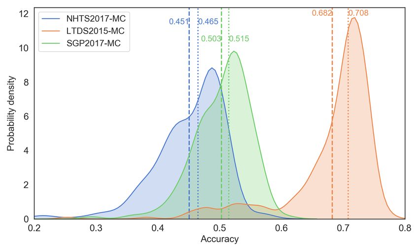
5.2. Hyper-dimension 2. datasets
The classifiers are further compared for each data set, given the large variations and the multi-
modal patterns illustrated in Figure 2. The prediction accuracy and ranking of the top 10 classifiers
and the three DCMs are presented in Table 3. The prediction accuracy in Table 3 represents the
average of the five-fold cross-validation for three sample sizes. The accuracy distributions of the
three datasets are visualized in Figure 5. The data-specific analysis yields the following four major
findings.
20You can also read


