Constraints and biases in a tropospheric two-box model of OH - Atmos. Chem. Phys
←
→
Page content transcription
If your browser does not render page correctly, please read the page content below

Atmos. Chem. Phys., 19, 407–424, 2019
https://doi.org/10.5194/acp-19-407-2019
© Author(s) 2019. This work is distributed under
the Creative Commons Attribution 4.0 License.

Constraints and biases in a tropospheric two-box model of OH
Stijn Naus1 , Stephen A. Montzka2 , Sudhanshu Pandey3,4 , Sourish Basu2,5 , Ed J. Dlugokencky2 , and Maarten Krol1,3,4
1 Meteorology    and Air Quality, Wageningen University and Research, Wageningen, the Netherlands
2 NOAA     Earth System Research Laboratory, Global Monitoring Division, Boulder, CO, USA
3 Institute for Marine and Atmospheric Research, Utrecht University, Utrecht, the Netherlands
4 Netherlands Institute for Space Research SRON, Utrecht, the Netherlands
5 Cooperative Institute for Research in Environmental Sciences, University of Colorado, Boulder, CO, USA

Correspondence: Stijn Naus (stijn.naus@wur.nl)

Received: 2 August 2018 – Discussion started: 16 August 2018
Revised: 21 November 2018 – Accepted: 5 December 2018 – Published: 11 January 2019

Abstract. The hydroxyl radical (OH) is the main atmo-           sitivity of interannual OH anomalies to the biases is mod-
spheric oxidant and the primary sink of the greenhouse gas      est (1 %–2 %), relative to the uncertainties on derived OH
CH4 . In an attempt to constrain atmospheric levels of OH,      (3 %–4 %). However, in an inversion where we implemented
two recent studies combined a tropospheric two-box model        all four bias corrections simultaneously, we found a shift
with hemispheric-mean observations of methyl chloroform         to a positive trend in OH concentrations over the 1994–
(MCF) and CH4 . These studies reached different conclusions     2015 period, compared to the standard inversion. Moreover,
concerning the most likely explanation of the renewed CH4       the absolute magnitude of derived global mean OH, and by
growth rate, which reflects the uncertain and underdeter-       extent, that of global CH4 emissions, was affected much
mined nature of the problem. Here, we investigated how the      more strongly by the bias corrections than their anomalies
use of a tropospheric two-box model can affect the derived      (∼ 10 %). Through our analysis, we identified and quanti-
constraints on OH due to simplifying assumptions inherent to    fied limitations in the two-box model approach as well as an
a two-box model. To this end, we derived species- and time-     opportunity for full 3-D simulations to address these limita-
dependent quantities from a full 3-D transport model to drive   tions. However, we also found that this derivation is an exten-
two-box model simulations. Furthermore, we quantified dif-      sive and species-dependent exercise and that the biases were
ferences between the 3-D simulated tropospheric burden and      not always entirely resolvable. In future attempts to improve
the burden seen by the surface measurement network of the       constraints on the atmospheric oxidative capacity through the
National Oceanic and Atmospheric Administration (NOAA).         use of simple models, a crucial first step is to consider and
Compared to commonly used parameters in two-box models,         account for biases similar to those we have identified for the
we found significant deviations in the magnitude and time-      two-box model.
dependence of the interhemispheric exchange rate, exposure
to OH, and stratospheric loss rate. For MCF these deviations
can be large due to changes in the balance of its sources and
sinks over time. We also found that changes in the yearly       1   Introduction
averaged tropospheric burden of CH4 and MCF can be ob-
tained within 0.96 ppb yr−1 and 0.14 % yr−1 by the NOAA         For the interpretation of atmospheric observations in the
surface network, but that substantial systematic biases exist   context of, for example, atmospheric pollution or in that
in the interhemispheric mixing ratio gradients that are input   of global warming, atmospheric models are often used. At-
to two-box model inversions.                                    mospheric models vary in complexity from simple one-box
   To investigate the impact of the identified biases on con-   models to state-of-the-art 3-D transport models. Different
straints on OH, we accounted for these biases in a two-box      types of models are suitable for addressing different types of
model inversion of MCF and CH4 . We found that the sen-         problems to different degrees of scrutiny. Therefore, there is
                                                                no model category that fits all problems. Simple box models

Published by Copernicus Publications on behalf of the European Geosciences Union.
408                                           S. Naus et al.: Constraints and biases in a tropospheric two-box model of OH

are easy to set up, computationally cheap, and transparent.        ies derived OH variations in a tropospheric two-box model
For these and other reasons, their use in atmospheric stud-        through an inversion of atmospheric MCF and CH4 obser-
ies is ubiquitous and has provided useful insights (e.g. Quay      vations (Rigby et al., 2017; Turner et al., 2017). In such an
et al., 1999; Walker et al., 2000; Montzka et al., 2011; Schae-    inversion, a range of parameters is optimized (most promi-
fer et al., 2016; Schwietzke et al., 2016). However, simple        nently emissions of MCF and CH4 and OH) so that the mod-
box models also put limitations on the derived results, as they    elled mixing ratios best match atmospheric observations of
are by definition less comprehensive than complex models.          the tracers involved.
For example, box models do not explicitly contain much in-            Both studies found that constraints on OH in this set-up
formation on a species’ spatial distribution, which can be im-     were weak enough that a wide range of OH concentration
portant if interacting quantities (e.g. loss processes) are dis-   variations over time and, by extent, CH4 emission scenarios
tributed non-homogeneously in space. Where exactly these           were possible as an explanation for the post-2007 increase
limitations lie and what the gain is from increasing model         in its measured global mole fraction. This is an important
complexity can be difficult to diagnose and depends on the         conclusion, because the CH4 growth rate, combined with the
application.                                                       CH4 lifetime (in turn dominated by MCF-derived OH), is
   A problem that has often been approached in box models is       generally assumed to provide the strongest top-down con-
that of constraining the global atmospheric oxidizing capac-       straints on global CH4 emissions and variations therein. We
ity, which is largely determined by the tropospheric hydroxyl      note that in Rigby et al. (2017) the two tropospheric boxes
radical (OH) concentration (Montzka et al., 2000; Montzka          were supplemented by a single stratospheric box, making it
et al., 2011). OH is dubbed the detergent of the atmosphere        technically a three-box model. However, due to our focus on
for its dominant role in the removal of a wide variety of          the troposphere, we hereafter treat this type of model, too, as
pollutants, including urban pollutants (CO, NOx ), green-          a two-box model, and where relevant we discuss the implica-
house gases (CH4 , HFCs), and HCFCs, which are green-              tion of the addition of a stratospheric box.
house gases, and also contribute to stratospheric ozone de-           There are two important reasons to approach the problem
pletion. The budgets of many of these pollutants have been         of constraining OH in a model of exactly two tropospheric
strongly perturbed since pre-industrial times, and it is impor-    boxes. Firstly, through the focus on annual timescales and
tant to understand what consequences this has had in the past,     hemispheric spatial scales, the result is only sensitive to in-
and could have in the future, for the atmosphere’s oxidizing       terannual variability in large-scale transport of the modelled
capacity.                                                          tracers. Moreover, by focusing on interannual variability as
   Due to its high reactivity, OH has a lifetime of seconds,       opposed to absolute OH or emission levels, remaining sys-
which inhibits extrapolation of direct measurements. More-         tematic offsets are not thought to significantly affect the out-
over, OH abundance is the net result of many different re-         come.
actions and reaction cycles, and thus modelling it process-           Secondly, a crucial part of the optimization consists of dis-
based in full-chemistry models is complex and dependent on         entangling the influence of OH and that of emission varia-
uncertain emission inventories of the many gases involved.         tions on observed MCF mixing ratios. Ideally, MCF emis-
Therefore, the most robust observational constraints on OH         sion variations would be prior knowledge. However, though
on the larger scales are thought to be derived indirectly from     MCF production is well documented, the emission timing is
its effect on tracers: gases that are predominantly removed by     much more uncertain (McCulloch and Midgley, 2001). MCF
OH. Depending on how well the tracer emissions are known,          was mainly used as a solvent in, for example, paint and de-
the time evolution of the global mixing ratio of such a tracer     greasers of metals. In these applications, MCF is released
can serve to constrain OH. The most well-established tracer        only when used, rather than when produced, which results in
for this purpose is methyl chloroform (MCF; e.g. Montzka           uncertainty in the emission timing. Moreover, due to the con-
et al., 2000; Bousquet et al., 2005). In part, this is because     tinuing decline of the atmospheric MCF mixing ratios, small,
it was identified early on as a tracer with a well-defined pro-    ongoing MCF emissions could eventually become important.
duction inventory that allowed emission estimates with small       Observation-inferred emissions exceeding bottom-up emis-
errors, relative to other gases (Lovelock, 1977; Prinn et al.,     sion inventories have been identified both from the US (Mil-
1987). Moreover, production of MCF was phased out in com-          let and Goldstein, 2004) and from Europe (Krol et al., 2003)
pliance with the Montreal Protocol, and the resulting rapid        as well as from other processes, such as MCF re-release from
drop in emissions made loss against OH the dominant term           the ocean (Wennberg et al., 2004). Therefore, in the absence
in the MCF budget (Montzka et al., 2011).                          of other constraints, emission uncertainties would limit the
   Research and debate surrounding OH (Krol and Lelieveld,         use of MCF for deriving interannual variability of OH. How-
2003; Krol et al., 2003; Reimann et al., 2005; Prinn et al.,       ever, in a two-box set-up, an additional constraint is provided
2005; Rigby et al., 2013; McNorton et al., 2016) has lead to       by the IH mole fraction gradient of MCF. Emission invento-
considerable improvements in its constraints, for example, a       ries show that MCF emissions are predominantly located in
likely upper bound on global interannual variability of OH         the Northern Hemisphere (NH), whereas OH has a NH to
of a few percent (Montzka et al., 2011). Two recent stud-          SH ratio that is uncertain, but the ratio has a likely range of

Atmos. Chem. Phys., 19, 407–424, 2019                                                www.atmos-chem-phys.net/19/407/2019/
S. Naus et al.: Constraints and biases in a tropospheric two-box model of OH                                                   409

0.80 to 1.10 (Montzka et al., 2000; Patra et al., 2014). This      a quantitative estimate of the impact of biases in a two-box
means that emission variations have a strong effect on the IH      inversion and to explore if and how these can be accounted
mole fraction gradient of MCF, whereas the effect of large-        for. Though this study is focused on the problem of OH, it
scale OH variations is much weaker. Thus, the IH gradient is       also serves as a case study of potential pitfalls in two-box
an important piece of information that can help to disentan-       models in general, when applied to interpreting global-scale
gle the influence of emissions from the influence of OH on         atmospheric observations.
MCF growth rate variations. This use of the IH gradient for
constraining global emissions of anthropogenically emitted
gases has also been recognized in previous research (Liang         2     Methods
et al., 2017; Montzka et al., 2018).
   Despite the appealing degree of simplicity offered by the       2.1    Two-box inversion
two-box model, its results still hinge on many simplifying
                                                                   In this section, we discuss the set-up of our two-box model
assumptions, both explicit (e.g. interhemispheric transport)
                                                                   inversion. The model incorporated two tracers (MCF and
and implicit (e.g. intrahemispheric transport). In this context,
                                                                   CH4 ) and consisted of two boxes (the troposphere in the NH
the uncertain outcome of the two recent two-box model stud-
                                                                   and in the SH), which were delineated by the Equator, i.e. it
ies puts forward an important question: how do the simpli-
                                                                   is fixed in time. The stratosphere was implicitly included in
fying assumptions inherent to the two-box set-up affect the
                                                                   the model through a first-order loss process that was taken to
conclusions drawn from it? Or, conversely, would these con-
                                                                   be equal for both hemispheres. The governing equations for
clusions change when moving the analysis to a 3-D trans-
                                                                   a tracer mixing ratio X are given in Eq. (1).
port model? A recent study (Liang et al., 2017) partly ex-
plored these questions. The study investigated how to incor-
porate information from 3-D transport models in a two-box          dXNH
model to increase the robustness of two-box model-derived               = ENH − (kOH [OH]NH + lstrat + lother )XNH
                                                                    dt
constraints on OH. They found that there are key parameters             − kIH (XNH − XSH ),                                   (1a)
in the two-box model that can be tuned to better represent the
                                                                   dXSH
3-D simulation results and thus ideally better represent atmo-          = ESH − (kOH [OH]SH + lstrat + lother )XSH
spheric transport in general. For example, they found that IH       dt
transport rates can be species-dependent.                               + kIH (XNH − XSH ).                                   (1b)
   Here, we provide a different approach to the issue. In the
first part of our study, we parametrized results from the 3-D         Thus, within each hemisphere, there were emissions (E),
global transport and chemistry model TM5 into a two-box            loss to OH (kOH [OH]X), loss to the stratosphere (lstrat X),
model. Through this parametrization, we explored difficul-         loss to other processes (lother X; e.g. ocean deposition), and
ties in the translation from the “reality” of a 3-D transport      transport between the hemispheres (kIH (XNH − XSH )). The
model to a two-box model and the assumptions made in the           model ran at an annual time step. The fundamentals of this
process. We focused on four aspects of the parametrization.        model set-up are also found in Rigby et al. (2017) and Turner
   Firstly, we investigated the tracer-dependent nature of IH      et al. (2017), though the exact treatment of the different bud-
transport as reported by Liang et al. (2017). Secondly, we         get terms can differ. For example, Turner et al. (2017) com-
analysed the IH OH ratio. Previous research has shown that         bined all tropospheric loss, including loss to the stratosphere,
because of tracer-specific source–sink distributions, different    in one term, whereas Rigby et al. (2017) included a strato-
tracers can be exposed to different global mean OH con-            spheric box, so that stratospheric loss becomes a transport
centrations (Lawrence et al., 2001). We extended this ob-          rather than a first-order loss term. Where relevant, we point
servation to a species-dependent IH OH ratio. Thirdly, we          out further differences with these previous studies.
looked at the stratospheric loss for MCF specifically. This net       Since the objective was to leverage observed mixing ra-
loss to the stratosphere might be slowing after its emissions      tios to infer information on tropospheric OH, we also set
dropped (Krol and Lelieveld, 2003; Bousquet et al., 2005).         up an inverse estimation framework, complementary to the
Fourthly, we used the 3-D simulation to investigate differ-        above forward model. The objective of the inversion was to
ences between the burden seen by the surface measurement           optimize a state x, such that the forward model best repro-
network of the National Oceanic and Atmospheric Adminis-           duced the observations without straying too far from a first
tration Global Monitoring Division (NOAA-GMD) and the              best guess: the prior. Therefore, the state is the vector which
true tropospheric and hemispheric burden in our 3-D model,         contains all parameters that needed to be optimized. The opti-
a bias that was also discussed in Liang et al. (2017).             mization objective is analogous to minimizing the cost func-
   In the second part of this study, we assessed the impact        tion J , as defined in Eq. (2):
of these four potential biases on derived OH variations in a
two-box inversion set-up that is very similar to Rigby et al.             1
(2017) and Turner et al. (2017). The objective was to provide      J (x) = (x − x prior )T B−1 (x − x prior )
                                                                          2

www.atmos-chem-phys.net/19/407/2019/                                                   Atmos. Chem. Phys., 19, 407–424, 2019
410 S. Naus et al.: Constraints and biases in a tropospheric two-box model of OH
1
+ (Hx − y)T R−1 (Hx − y), (2) and, in the optimization,
2
i i i i i
PRap = (1 − fMed − fSlow − fStock )PRap, prior ,
when B and R are the prior and observation error covariance
matrices respectively, H is the forward model, and y is the i i i i
PMed = PMed, prior + fMed PRap, prior ,
observation vector. In addition, we compute the cost function i i i i
PSlow = PSlow, prior + fSlow PRap, prior ,
gradient ∇J (Eq. 3).
i i i i
PStock = PStock, prior + fStock PRap, prior . (6)
∇J (x) = B−1 (x − x pri ) + HT R−1 (Hx − y), (3) An important choice in the inversion set-up is which pa-
rameters to prescribe and which to optimize. Rigby et al.
with HT the transpose of the forward model, also known (2017) optimized all parameters, so as to explore the full
as the adjoint model. Note that because the forward model uncertainty of the optimization within the inversion frame-
H was non-linear (e.g. OH chemistry), we used the ad- work. Turner et al. (2017) only optimized hemispheric MCF
joint of the tangent-linear forward model. Calculation of the and CH4 emissions and hemispheric OH, while the remain-
cost function gradient facilitates quicker convergence of the ing uncertainties were partly explored in sensitivity tests. We
optimization. For the minimization we used the Broyden– choose to optimize four end products for each year: global
Fletcher–Goldfarb–Shanno algorithm. In essence, this sta- OH, global MCF emissions, global CH4 emissions, and the
tistical inversion set-up is the same as that used in the CH4 emission fraction in the NH. Thus we had a closed sys-
4DVAR system of ECMWF (Fisher, 1995) and TM5-4DVAR tem, as we also fitted to four observations: the global mean
(Meirink et al., 2008). mixing ratio and the IH gradient of both MCF and CH4 .
For the optimization of MCF emissions, we used an ex- In addition to the 4DVAR inversion, we generated a Monte
tended version of the emission model from McCulloch and Carlo ensemble, where in each realization, the prior and the
Midgley (2001). This emission model was adopted to ac- observations were perturbed, relative to their respective un-
count for the varying and uncertain release rates of MCF certainties. Then, the new prior was optimized using the new
when used in different applications (e.g. degreasing agent observations. The Monte Carlo simulation quantified the sen-
or paint). This uncertainty results in a gap between the un- sitivity of the optimization to the prior choice and to the real-
certainty in production, or integrated emissions (∼ 2 %), and ization of the observations. The Monte Carlo set-up also al-
the uncertainty in annual emissions (up to 40 %; McCulloch lowed us to explore the sensitivity of the inversion to param-
and Midgley, 2001). Therefore, production was distributed eters that were not optimized, such as the fraction of MCF
between four different categories with different release rates: emissions in the NH. This approach had the added advan-
rapid, medium, slow, and stockpile. In the prior distribution, tage that parameters that were perturbed in the Monte Carlo
the bulk of production (> 95 %) was placed in the rapid cat- simulation, but not optimized in the 4DVAR system, did not
egory. To account for uncertainty in the production inven- need to have a Gaussian error distribution. Gaussian proba-
tory, we also adopted an additional emission term superim- bility distributions are normally a prerequisite in a 4DVAR
posed on the production-derived emissions. The emissions inversion. The specifics of our inversion set-up are given in
in year i were then given by Eqs. (4) and (5). For each year Table 1.
i, we optimized four parameters for MCF emissions: three
parameters that shifted emissions between the rapid produc- 2.2 TM5 set-up and two-box parametrizations
i
tion category and each of the other three categories (fMedium ,
i i
fSlow , and fStock in Eq. 6) and the additional emissions term 2.2.1 3-D model set-up
i
(EAdditional ), which had an uncertainty constant through time.
This emission model is similar to that used in Rigby et al. For the 3-D model simulations we used the atmospheric
(2017), though ours leaves more freedom with respect to the transport model TM5 (Krol et al., 2005). The model was op-
timing of emissions. erated at a 6◦ × 4◦ horizontal resolution, at 25 vertical hy-
brid sigma-pressure levels. The simulation period was 1988–
2015, where we treated 1988 and 1989 as spin-up years.
E i = ERap
i i
+ EMed i
+ ESlow i
+ EStock i
+ EAdditional (4) TM5 transport was driven by meteorological fields from the
ECMWF ERA-Interim reanalysis (Dee et al., 2011). Convec-
for the emissions in year i, where
tion of tracer mass was based on the entrainment and detrain-
i i i−1 ment rates from the ERA-Interim dataset. This is an update
ERap = 0.75PRap + 0.25PRap ,
i i i−1
from the previous convective parametrization used by, for ex-
EMed = 0.25PMed + 0.75PMed , ample, Patra et al. (2011). The new convective scheme results
i i−1 i−2 in faster interhemispheric exchange of tracer mass, more in
ESlow = 0.25PSlow + 0.75PSlow ,
11 line with observations (Tsuruta et al., 2017).
i−j
X
i
EStock = PStock , (5) We ran TM5 with three tracers: CH4 , MCF, and SF6 . For
j =1 CH4 , we annually repeated the 2009–2010 a priori emission
Atmos. Chem. Phys., 19, 407–424, 2019 www.atmos-chem-phys.net/19/407/2019/S. Naus et al.: Constraints and biases in a tropospheric two-box model of OH 411
Table 1. The relevant settings we used in the inversion of our two-box model. The upper section contains the parameters optimized in
the inversion, which were also perturbed in the Monte Carlo ensemble. These parameters have Gaussian uncertainties, and their mean and
1σ uncertainty are given. The middle section contains parameters that were perturbed in the Monte Carlo, but not optimized. The middle
parameters have uniform uncertainties, of which the lower and upper bound are given. The bottom section contains parameters that were
neither optimized nor perturbed. For these parameters, the left column gives the standard setting, whereas the alternative column indicates
whether we also ran an inversion using a TM5-derived time series (see Sect. 2.2.2).
Parameters optimized in inversion and perturbed in the Monte Carlo ensemble (Gaussian)
Parameter Prior estimate Uncertainty
Global MCF emissions Based on
McCulloch and Midgley (2001)
– fMedium 0% 5%
– fSlow 0% 5%
– fStock 0% 5%
– Unreported emissions 0 Gg yr−1 10 Gg yr−1
Global CH4 emissions 550 Tg yr−1 15 %
Global OH 9 × 10⁵ molec cm−3 10 %
Fraction NH CH4 emissions 75 % 10 %
Parameters not optimized in inversion, but perturbed in the Monte Carlo ensemble (uniform)
Parameter Lower bound Upper bound
Fraction NH MCF emissions 90 % 100 %
Parameters not optimized in inversion and not perturbed in the Monte Carlo ensemble
Parameter Standard Alternative
Interhemispheric OH ratio 0.98 TM5 derived∗
MCF lifetime with respect to 83 yr –
oceanic loss
MCF lifetime with respect to 45 yr TM5 derived∗
stratospheric loss
CH4 lifetime with respect to 150 yr TM5 derived∗
stratospheric loss
Interhemispheric transport 1 yr−1 TM5 derived∗
∗ see Sect. 2.2.2.
fields used by Pandey et al. (2016), and we also used the TransCom Age of Air project (Krol et al., 2018), with no loss
same fields for stratospheric loss to Cl and O(1 D). For MCF, process implemented.
we used emissions from the TransCom-CH4 project (Patra Since the above set-up is simplistic in some aspects (e.g.
et al., 2011). Since these emissions were available only up annually repeating CH4 emissions), we also ran a “nudged”
to 2006, we assumed a globally uniform exponential decay simulation. In the nudged simulation, we scaled the mixing
of 20 % yr−1 afterwards, similar to Montzka et al. (2011). ratios of a tracer up or down in latitudinal bands, depend-
MCF-specific loss fields (ocean deposition and stratospheric ing on the mismatch of the model with NOAA observations
photolysis) were also taken from the TransCom-CH4 project. (analogous to Bândă et al., 2015), with a relaxation time of
Details of the MCF loss and emission fields can be found 30 days. This method ensured that the model followed the
in the TransCom-CH4 protocol (http://transcom.project.asu. long-term trend in observations without requiring a full in-
edu/pdf/transcom/T4.methane.protocol_v7.pdf, last access: version. The nudged simulation provided a test of the sensi-
1 September 2018). The OH loss fields we used were a com- tivity of our results to the source–sink distributions we used
bination of the 3-D fields from Spivakovsky et al. (2000) in in the 3-D simulation.
the troposphere and stratospheric OH as derived using the 2-
D MPIC chemistry model (Brühl and Crutzen, 1993). The 2.2.2 Parametrizing 3-D model output to two-box
OH fields were scaled by a factor 0.92, as described by Hui- model input
jnen et al. (2010). For SF6 , we used emission fields from the
Here we outline how we used the TM5 simulations to de-
rive two-box model parametrizations for stratospheric loss
www.atmos-chem-phys.net/19/407/2019/ Atmos. Chem. Phys., 19, 407–424, 2019412 S. Naus et al.: Constraints and biases in a tropospheric two-box model of OH
(lstrat ) and for interhemispheric exchange (kIH ). Firstly, the the data are aggregated to two hemispheric averages, as in a
3-D fields were divided into three boxes: the troposphere in two-box model, quantification of the potential biases is cru-
the NH and in the SH and the stratosphere. The border be- cial.
tween the hemispheres was taken as the Equator, fixed in We explored the resulting bias in our model framework.
time. Where relevant we discuss the sensitivity of our results By subsampling the TM5 output at the locations of NOAA
to this demarcation. We defined a dynamical tropopause as stations, at NOAA measurement instances, we generated a
the lowest altitude where the vertical temperature (T ) gradi- set of model-sampled observations. These model-sampled
ent is smaller than 2 K km−1 , clipped at a geopotential height observations were intended to be as representative as pos-
of 9 and 18 km. Our analysis was found to be insensitive to sible for the real-world observations of the NOAA network.
the exact definition of the tropopause. Next, we computed an To aggregate the station data to hemispheric averages, we
annual budget for each box. For the two tropospheric boxes, used methods similar to those deployed by NOAA (for MCF,
this was done as in Eq. (1). This was supplemented by Eq. (7) Montzka et al., 2011, with further details on our adaption
for the stratospheric box. in Sect. S1 in the Supplement; for CH4 , Dlugokencky et al.,
1994). Hemispheric averages for CH4 were derived from 27
sites and MCF averages from 12 sites. By comparison of the
dXStrat
= −LStrat
local + lstrat (XSH + XNH ), (7) resulting products with the calculated tropospheric burden,
dt as derived from the full tropospheric mixing ratios, we could
where emissions, local loss, and mixing ratios per box assess how well the burden derived from the NOAA net-
could be derived from the 3-D model in- and output, and thus work represents the model-simulated tropospheric burden.
lstrat and kIH could be inferred from these equations. Note that The two end products we investigated for each tracer were
we did not strictly need the stratospheric budget equation to the rate of change of the global mean mixing ratio and that
resolve two parameters, but we used it to resolve numeri- of the IH gradient. Note that by mixing ratio we mean the
cal inaccuracies. Resolving the budget of each species in this dry air mole fraction. These two parameters best reflect the
manner provided the necessary input of the tropospheric two- information as it is used in a two-box model; the global mean
box model defined in Sect. 2.1 such that on the hemispheric mixing ratio is used to constrain the combined effect of OH
and annual scale, identical results were obtained with the 3-D and emissions, while the IH gradient is used to distinguish
and the two-box models. between the two. Note that in previous box-model studies of
An additional parameter that we derived from the TM5 MCF, often only global growth rates were derived (Montzka
simulations was the IH OH ratio to which each tracer was et al., 2000; Montzka et al., 2011).
exposed. We quantified this parameter as the ratio between
hemispheric lifetimes with respect to OH (τOH ): 2.3 Potential biases in the two-box model
SH
τX, By concentrating on the budget of MCF, we identified three
OH
rLOH = NH
. (8) parameters that need attention in the two-box model: IH
τX, OH transport, the IH OH ratio, and loss of MCF to the strato-
Note that this ratio might differ from the physical IH OH sphere. In addition, we investigated the potential bias in con-
ratio because of correlations between the tracer distribution, verting station data to hemispheric averages (see Sect. 2.2.3
the OH field, and the temperature distribution. and S1). We quantified these biases and propagated them in
two-box model inversions, as discussed in Sect. 3.2, to quan-
2.2.3 Model-sampled observations tify their impact on derived quantities related to OH.
The standard in tracking global trends in atmospheric trace Interhemispheric transport
gases are surface measurement networks. For CH4 and MCF
these are most notably the NOAA-GMD (Dlugokencky et al., IH transport of tracer mass can vary because of variations
2009; Montzka et al., 2011) and the AGAGE (Advanced in IH transport of air mass (e.g. influenced by the El Niño–
Global Atmospheric Gases Experiment; Prinn et al., 2018) Southern Oscillation, particularly at Earth’s surface; Prinn
networks. By selecting measurement sites far removed from et al., 1992; Francey and Frederiksen, 2016; Pandey et al.,
sources, the theory is that a small number of sites already puts 2017) or because of variations in the source–sink distribu-
strong constraints on the global growth rate (Dlugokencky tion and thus of the tracer’s concentration distribution itself.
et al., 1994). In general, quantification of the robustness of Generally, interannual variability in IH transport is consid-
the derived growth rates based solely on observations can be ered to be on the order of 10 % (Patra et al., 2011). Two-box
difficult, since there are likely systematic biases inherent to model studies typically assume time-invariant IH exchange
sampling a small number of surface sites. When assimilated (Turner et al., 2017) and/or similar exchange rates for differ-
into a 3-D transport model, these biases will largely be re- ent tracers (Rigby et al., 2017). Here we investigated whether
solved (if transport is correctly simulated). However, when such assumptions hold for a tracer which undergoes strong
Atmos. Chem. Phys., 19, 407–424, 2019 www.atmos-chem-phys.net/19/407/2019/S. Naus et al.: Constraints and biases in a tropospheric two-box model of OH 413
source–sink redistributions over time, such as MCF. The IH Lelieveld, 2003; Bousquet et al., 2005). We will investigate
transport variations we derived for each tracer are discussed this possibility in Sect. 3.1.4.
in Sect. 3.1.1.
2.4 Standard two-box inversion and bias correction
Surface sampling bias
To assess the impact of the biases discussed in Sect. 2.3 on a
As discussed in Sect. 2.2.3, we explored the bias that results two-box model inversion, we ran our inversion (see Sect. 2.1)
from representing hemispheric averages using sparse surface using different settings. In the standard, default inversion,
observations. Surface networks are a valuable resource, be- we did not consider any of the four biases discussed above.
cause they provide high-quality, long-term measurements of Thus, we used constant IH exchange (1 year), constant strato-
a growing variety of tracers. However, temporal, horizon- spheric loss of MCF (45 years), and a constant IH OH ratio
tal, and vertical coverage of surface networks is limited. In (0.98; see Table 1). The first three potential bias corrections
Sect. 3.1.2 we discuss how these limitations can result in bi- were then straightforwardly implemented by replacing these
ases in two-box model observations. constant values with the time series we derived for each pa-
rameter from the full 3-D simulations (details in Sect. 2.2.2).
The interhemispheric OH ratio As mentioned in Sect. 2.1, the inversion did not include un-
certainties in these three parameters. We did this because
The IH ratio of OH concentrations is an uncertain parameter. conventional uncertainties tend to be large, therefore includ-
This is mostly because of a mismatch between results from ing them would have attenuated the impact of the bias cor-
full-chemistry models (1.13–1.42; Naik et al., 2013) and rections, while the corrections were the main interest of this
from MCF-derived constraints (0.80–1.10; Brenninkmeijer comparison. For the surface sampling bias, we first computed
et al., 1992; Montzka et al., 2000; Patra et al., 2014). The a correction between the hemispheric means as derived from
latter is generally the loss ratio considered in two-box mod- the model-sampled observations and the calculated (TM5)
els (1.0 in Turner et al., 2017, and 0.95–1.20 in Rigby et al., hemispheric, tropospheric means (with demarcation at the
2017) and is similar to the ratio we used in the TM5 sim- Equator). Then, we applied this correction to the real-world
ulations (0.98 Spivakovsky et al., 2000). However, the bias NOAA hemispheric means we used in the standard inversion.
we consider here is of a different nature; it is the difference This gave a new set of observations, which we used in the in-
between the physical IH OH ratio and the IH loss ratio a par- version (discussed in Sect. 3.1.2). Both the standard and the
ticular tracer is exposed to. It is known that different tracers corrected set of observations are shown in Fig. 1. Through
can be exposed to different oxidative capacities (Lawrence comparison of the results of the standard inversion and of an
et al., 2001). Therefore, different tracers might similarly be inversion with one or more biases implemented simultane-
influenced by different IH ratios in OH. We explore this bias ously, we can evaluate the individual and cumulative impact
in Sect. 3.1.3. of the biases on derived OH and CH4 emissions.
MCF loss to the stratosphere
3 Results
The second-most important loss process of MCF is strato-
spheric photolysis. In our TM5 set-up, this loss process re- 3.1 Biases
sulted in an in-stratosphere lifetime (stratospheric burden di-
vided by stratospheric loss) of 4 to 5 years. It is generally 3.1.1 Interhemispheric transport
assumed that this in-stratosphere loss translates to a global
lifetime of MCF with respect to the stratosphere (global bur- The IH exchange coefficients, derived for the three differ-
den divided by stratospheric loss) of 40 to 50 years (Naik ent tracers as described in Sect. 2.2.2, are shown in Fig. 2.
et al., 2000; Chipperfield and Liang, 2013), which corre- Clearly, the exchange rates differ between tracers both in
sponds to ∼ 10 % of global MCF loss. Rigby et al., 2017 mean value as well as in interannual variability. MCF is the
assumed a time-invariant in-stratosphere lifetime, but due clear outlier, but SF6 and CH4 also show different variations.
to the inclusion of a stratospheric box, the global lifetime The drivers of these differences are differences in intrahemi-
with respect to stratospheric loss could vary somewhat due spheric tracer distributions and in the underlying source and
to changes in the troposphere–stratosphere gradient. These sink distributions. The three tracers differ strongly in this re-
variations were tuned to result in a global lifetime with re- spect; SF6 and MCF are emitted almost exclusively in the
spect to stratospheric loss of 40 (29–63) years. Turner et al. NH mid-latitudes, whereas CH4 has significant emissions in
(2017) incorporated this loss process in the OH loss term. the tropics and in the SH. SF6 has no sink implemented in
Due to the rapid drop in MCF emissions and the relatively our simulations, whereas MCF and CH4 have a sink with a
slow nature of troposphere–stratosphere exchange, this life- distinct tropical maximum in OH. This all affects how IH
time could vary through time (Montzka et al., 2000; Krol and transport of air mass translates to IH transport of tracer mass.
www.atmos-chem-phys.net/19/407/2019/ Atmos. Chem. Phys., 19, 407–424, 2019414 S. Naus et al.: Constraints and biases in a tropospheric two-box model of OH
Figure 1. Hemispheric, annual mean time series of CH4 (a) and MCF (b), as derived from the NOAA surface sampling network (for CH4 ,
27 sites were used; for MCF, 12 sites were used). Solid lines denote averages as derived directly from the NOAA surface sampling network
(which are used in our standard inversion). Dashed lines denote the same time series, but those that are adjusted by correction factors that
were derived from our TM5 simulations. The correction factors reflect the differences between hemispheric averages based on model-sampled
observations and hemispheric averages derived from the full TM5 troposphere. Figure 3 shows the ratios between the standard and corrected
time series.
in the pattern of IH transport which favours IH exchange of
CH4 and SF6 . It is unclear from this analysis what the under-
lying mechanism is exactly, except that it is driven by tem-
poral variations in transport, thus there are parameters in the
meteorological fields which also show a trend; otherwise this
final product cannot exhibit a trend. However, it might be that
the sensitivity of TM5 transport to these parameters is biased.
To test the sensitivity of the derived IH exchange rates to
the source–sink distribution, we compared kIH derived from
the standard simulation to the nudged simulation (the nudg-
Figure 2. The IH exchange rate for MCF, CH4 , and SF6 , as derived ing procedure is explained in Sect. S2). IH transport of CH4
from a TM5 simulation (see Sect. 2.2.2). as derived from the nudged simulation showed higher inter-
annual variations than in the standard simulation (more dis-
cussion in Sect. S4), which can be expected, as the source–
Most notable is the minimum in the IH exchange rate for sink distribution becomes more variable. However, the gen-
MCF in the 2000–2005 period. The timing of the 1989–2003 eral characteristics were conserved; most notably, the posi-
decline in kIH coincides with the initial drop in MCF emis- tive trend over the entire period persisted, for CH4 and for
sions. An important shift in the distribution of the MCF mix- SF6 . For MCF, we find that the general characteristics of de-
ing ratio is that the global minimum shifts from the South rived kIH are similarly insensitive to nudging, with the main
Pole to the tropics. In the same period, there is a strong change being a deeper 2000–2005 minimum in the nudged
vertical redistribution which has also likely impacted IH ex- simulation. In the end, we deem the anomalies presented in
change. It is not obvious that these changes should result in Fig. 2 to be quite robust with respect to the spatio-temporal
slower IH exchange, but in the end, in TM5, they do. source–sink distribution.
Another notable feature is the positive trend in the IH ex- When the hemispheric interface is shifted from the Equa-
change rate for CH4 (+0.35 ± 0.05 % yr−1 ; p = 0.00) and tor to 8◦ N, which is more representative of the average posi-
for SF6 (+0.50 ± 0.01 % yr−1 ; p = 0.00). For CH4 , we used tion of the Intertropical Convergence Zone (ITCZ), the IH
annually repeating sources, whereas for SF6 we included exchange rate increases for all tracers, but the variability
emission variations (see Sect. 2.2). This means that for CH4 , in IH exchange of CH4 and SF6 remains largely unaffected
changes in the source–sink distribution did not contribute to (see Sect. S4). However, for MCF, the variability shifts com-
the trend or to the variability. Indeed, in a simulation with an- pletely. Rather than decreasing after the emission drop, the
nually repeating meteorology, we found near-zero variability IH exchange rate now increases. This sensitivity reflects that
in kIH for CH4 (see Sect. S4). Therefore, there is something for a tracer with a relatively small IH gradient which min-
in the combination of the meteorological data, the treatment imizes in the tropics, it becomes difficult to define an IH
of this data in TM5, and the source–sink distribution of both transport rate in a two-box model. By extension, care should
CH4 and SF6 which resulted in a significantly positive trend be taken when interpreting the IH gradient of MCF in later
in the IH exchange rate of both gases. This trend could either years, since the influence of IH transport is difficult to iso-
indicate an acceleration of IH transport of air mass or a shift
Atmos. Chem. Phys., 19, 407–424, 2019 www.atmos-chem-phys.net/19/407/2019/S. Naus et al.: Constraints and biases in a tropospheric two-box model of OH 415
Table 2. Mean observational errors as derived from TM5 simu- for MCF. The trend in the IH bias of MCF became smaller
lations over the 1994–2015 period. The errors were quantified as but persisted.
the mean difference between annual means derived from model- Liang et al. (2017) performed a similar analysis for MCF.
sampled observations and annual means derived from the full tro- They reported a similar low-to-absent bias in the global
pospheric grid. CH4 uncertainties are given both in ppb yr−1 and mean and a more significant bias in the IH gradient of MCF
relative to the global mean mixing ratio. Uncertainties for MCF are
(∼ 10 %). This is smaller than the bias we found, even if we
only given relative to the global mean because of its strong temporal
decline.
demarcated the hemisphere at 8◦ N. However, an important
difference is that in Liang et al. (2017), model-sampled ob-
Global IH gradient servations were compared to the surface grid, instead of to
growth rate rate of change the full troposphere. Thus, their bias estimate did not include
CH4 0.96 ppb yr−1 / 0.05 % yr−1 2.56 ppb yr−1 / 0.13 % yr−1 vertical effects. When we used the surface grid as a reference,
MCF – / 0.14 % yr−1 – / 0.33 % yr−1 the IH bias for CH4 was reduced to −10 %, i.e. it reversed.
For MCF the bias shift persisted, and the maximum bias was
only slightly reduced to 15 %, indicating a dominant influ-
late. Sensitivities in the derivation of the IH exchange rate ence from the latitudinal dimension. We emphasize that for
are discussed in more detail in Sect. S4. a tropospheric two-box model, the comparison with the full
troposphere is most relevant.
3.1.2 Surface sampling bias This analysis also provided an estimate of uncertainties
in the rate of change of the global mixing ratio and in that
Figures 1 and 3 show the surface network bias in the global of the IH gradient: the relevant observational parameters in
mean mixing ratios and in the IH gradient. In Fig. 3, the a two-box inversion. Table 2 gives the differences between
bias is quantified as the ratio between values derived from the quantities derived from model-sampled observations and
the model-sampled observations (see Sect. 2.2.3) and values from the full troposphere, i.e. the “true” (TM5) error. We can
derived from the hemispheric (TM5) troposphere. A compar- compare this TM5-derived uncertainty to uncertainties de-
ison with global mean mixing ratios derived from real-world rived only from observations, which we used in the two-box
NOAA observations is given in Sect. S2. inversions. For CH4 , we used uncertainties as reported by
The bias in the IH gradient was particularly large, be- NOAA. These were obtained by generating an ensemble of
cause averages based on NOAA surface stations systemati- surface network realizations, where in each realization dif-
cally overestimated the tropospheric burden in the NH and ferent sites are excluded or double-counted randomly (boot-
underestimated the burden in the SH. Two important effects strapping). For each realization, aggregated quantities such
contributed to this bias. Firstly, in the NH, where most emis- as the global mean growth rate can be derived. The spread
sions were located, mixing ratios tended to decrease with al- within the ensemble then provides a measure for the uncer-
titude, while in the SH vertical gradients were much smaller tainty. For MCF no such uncertainties are reported. There-
or even reversed. Secondly, latitudinal gradients of both MCF fore, we developed our own method, which is described in
and CH4 tended to be highest in the tropics, where few or no Sect. S1.
measurement sites were available. Again, due to high emis- Following these methods, we found observation-derived
sions in the NH, mixing ratios in the NH decreased towards uncertainties in the global mean growth rate of around
the Equator, while mixing ratios increased towards the Equa- 0.60 ppb yr−1 and 0.6 % yr−1 for CH4 and for MCF respec-
tor in the SH. Both biases were of the opposite sign in each tively. NOAA does not report an uncertainty in the IH gra-
hemisphere. Thus, in a global average, these biases largely dient of CH4 , but error propagation from hemispheric means
cancelled, and only a small overestimate remained (Fig. 3a). gave an uncertainty of 1.1 ppb yr−1 . For MCF, we found a
For the IH gradient, however, these biases added up, which time-dependent uncertainty in the rate of change of the IH
resulted in an overestimate of the IH gradient by surface sta- gradient of 1.0 %–1.5 %.
tions of up to 20 %–40 % (Fig. 3b). For MCF before 1995 and The CH4 errors we derived from the TM5 simulation were
for CH4 throughout the analysis period, the bias from the ver- slightly higher than the uncertainties reported by NOAA.
tical gradient dominated. The shift in the bias for MCF was Furthermore, since we used annually repeating CH4 emis-
driven by a shift in the latitudinal gradient. The IH gradient sions, variations in CH4 emissions can further increase the
of MCF got a minimum in the tropics, and apparently this ex- error. Indeed, the nudged run (see Sect. S2) resulted in 20 %
acerbated the effect of the lack of tropical stations, combined higher uncertainties. However, it is important to note that the
with the simple, linear latitudinal interpolation we adopted CH4 uncertainties reported by NOAA are intended to reflect
for MCF (see Sect. S1). the match with the marine boundary layer (MBL), rather than
We note that the derived bias in the IH gradient is sensitive with the full troposphere. Therefore, it is not surprising that
to the demarcation of the two tropospheric boxes. When we the errors we find are somewhat higher.
shifted the IH interface from the Equator to 8◦ N, the bias was For MCF, we adopted observation-derived uncertainties
reduced to 15 % for CH4 and varied between 15 % and 25 % that were significantly lower than those used by Rigby et al.
www.atmos-chem-phys.net/19/407/2019/ Atmos. Chem. Phys., 19, 407–424, 2019416 S. Naus et al.: Constraints and biases in a tropospheric two-box model of OH
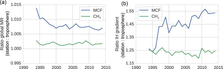
Figure 3. The surface sampling bias in the global mixing ratio (MR) (a) and in the IH gradient (b) of MCF and of CH4 . The bias was
quantified as the ratio between values derived from the NOAA surface sampling network and values derived from the full (TM5) troposphere.
The biases were derived from 27 and 12 sites for CH4 and for MCF, respectively. Figure 1 visualizes the impact of correcting for the sampling
bias in real-world NOAA observations.
(2017) and Turner et al. (2017); both studies reported uncer-
tainties of around 5 % in hemispheric averages. Both studies
used different methods that were grounded on different ob-
servational information. In Rigby et al. (2017), temporal vari-
ability dominated the uncertainty estimate, while in Turner
et al. (2017) spatial variations were used. Our method is more
similar to Rigby et al. (2017) but with modifications that av-
eraged out some of the temporal variability, under the as-
sumption that variability at different measurement sites was
largely uncorrelated (details in Sect. S1). This shows that
observation-derived uncertainties in MCF averages are un-
Figure 4. The ratio between tracer lifetime with respect to OH loss
certain quantities, in large part due to the relatively low num-
in the SH troposphere and NH troposphere (see Eq. 8). Additionally,
ber of available surface sites. Therefore, the uncertainty de-
the IH ratio in OH concentrations is shown.
rived from TM5 is an especially useful addition for MCF.
Table 2 shows that TM5-derived uncertainties in MCF av-
erages are significantly lower than all observation-derived it did not explain the difference between the IH loss and the
estimates. This result indicates that even the use of a sim- IH OH ratio. Instead, we found that the systematic positive
ple averaging algorithm and a small number of surface sites, offset was largely driven by an IH asymmetry in the spatio-
relative to what is available for CH4 , already results in temporal correlations between OH and temperature. Mostly,
well-constrained hemispheric and global growth rates for this was because the OH maximum in the NH was located at
MCF. The TM5-derived estimate thus supports the use of lower altitude than in the SH in our 3-D model. Since at low
our observation-derived uncertainty estimates, rather than the altitudes, temperatures are higher, and higher temperatures
higher estimates used in previous studies. correspond to higher reaction rates, this asymmetry resulted
in relatively high NH loss rates. As such, the ratio bias was
3.1.3 Interhemispheric OH ratio sensitive to the OH distribution used in the 3-D model simu-
lation.
In the TM5 simulations from which the global loss rates were The trend in the ratio for MCF was driven by the change
derived, the prescribed tropospheric OH fields were taken in the spatial distribution of MCF after the emission drop
from Spivakovsky et al. (2000). In these fields, the IH OH in the mid-1990s. Before the drop, the IH gradient of MCF
ratio is 0.98 when the IH interface is considered to be the was emission-driven and high (25 %). This resulted in a neg-
Equator. One might expect a similar ratio between OH loss ative correlation between OH / temperature and MCF in the
in the NH and in the SH, which we quantified through the IH NH, which drove the initially lower loss ratio. After the emis-
ratio in tracer lifetime with respect to OH loss (Eq. 8). We sion drop, the IH gradient became largely sink-dominated
found that this is not the case (see Fig. 4). and dropped to 3 %. The ratio then became similar, though
The loss ratio was up to 7 % higher than the physical OH not identical, to that of CH4 , which also has a relatively low
ratio. Moreover, the ratio was not the same for MCF and IH gradient (5 %). The exact reasons for the IH asymmetry in
CH4 , and the ratio that corresponded to MCF showed a trend. the OH loss rate were complex; further details are discussed
The IH asymmetry in temperature in our model was small, so in Sect. S3.
Atmos. Chem. Phys., 19, 407–424, 2019 www.atmos-chem-phys.net/19/407/2019/S. Naus et al.: Constraints and biases in a tropospheric two-box model of OH 417
to the troposphere (in the downward branch of the Brewer–
Dobson circulation; Butchart, 2014) that was exposed to
higher MCF emissions. Therefore, the delay between the two
opposed fluxes resulted in a reduced net upward flux rate in
an atmosphere with decreasing emissions compared to an at-
mosphere with increasing or constant emissions. Consistent
with this hypothesis, we found that the stratospheric loss rate
did not decrease in a TM5 simulation with MCF emissions
fixed at 1988 levels and that stratospheric loss did decrease,
but recovered, when we fixed emissions at 2005 levels over
the entire analysis period (results not shown). This also im-
Figure 5. The tropospheric loss rate to the stratosphere, as derived plies that the troposphere–stratosphere exchange will slowly
from the TM5 simulations (see Sect. 2.2.2).
recover when MCF emissions stop decreasing.
For CH4 , we found a stratospheric lifetime of 160–
The derived IH OH ratio was sensitive to the demarcation 170 years, similar to the range reported in Chipperfield and
of the two tropospheric boxes. When we shifted the position Liang (2013). For SF6 , there was no loss process imple-
from the Equator to 8◦ N, all IH OH ratios were reduced by mented in our model. However, storage of SF6 in the strato-
10 % to 15 %. However, the offset between the physical IH sphere acted as an effective sink to the troposphere, with a
OH ratio and the actual loss ratio remained similar, as did the lifetime of 100–160 years.
trend in the loss ratio for MCF.
3.2 Two-box inversion results
3.1.4 Loss to the stratosphere
In this section, we present a comparison between the results
Figure 5 shows the stratospheric loss rate, as derived from of the standard inversion and an inversion that incorporated
Eqs. (1) and (7). Most notably, the stratospheric loss rate the four bias corrections (referred to as “four biases”). The
showed a significant negative trend for MCF, decreasing by inversion set-ups are described in Sect. 2.4. The OH and
68 % from 1991 to 1997. The lifetime of MCF with respect CH4 emission anomalies of both inversions are presented in
to stratospheric loss, as calculated from TM5, was in 1990 Fig. 6, along with uncertainty envelopes of 1 standard de-
similar to the range reported in literature: 40 to 50 years viation. The envelopes are wide, and with respect to these
(Naik et al., 2000; Chipperfield and Liang, 2013). Afterwards envelopes there were no significant differences between our
however, the corresponding timescale for stratospheric loss two inversions. Interestingly, differences between the two in-
quickly increases. As loss to the stratosphere is a secondary versions were the smallest in the 1998–2007 period, during
loss process, it is generally assumed that variability in MCF which MCF is thought to provide the strongest constraint on
loss is driven predominantly by OH variations (Montzka OH (Montzka et al., 2011). Note that the final analysis period
et al., 2011; Turner et al., 2017; Rigby et al., 2017). Here, started from 1994 (rather than from 1990), because we only
we found that this is not necessarily the case. The decline had sufficient NOAA coverage of MCF available from 1994
in loss to the stratosphere was not an artefact resulting from onwards.
treating a transport process as a loss process; when taking the Shown in grey in Fig. 6 are the anomalies derived by Rigby
exchange proportional to the troposphere–stratosphere gradi- et al. (2017) (from the NOAA dataset) and by Turner et al.
ent, we still found a decrease in the exchange rate of 63 %. (2017). The four inversions showed qualitatively similar time
Previous research has identified that the tropospheric life- dependencies, and differences generally fell within 1 stan-
time with respect to stratospheric loss could be decreasing dard deviation and always within 2 standard deviations. Dif-
(Krol and Lelieveld, 2003; Prinn et al., 2005; Bousquet et al., ferences with Turner et al. (2017) are largest, most notably
2005), but not to the degree that we found here and not rela- after 2010, which can be expected since they use a combined
tive to the troposphere–stratosphere gradient. This is impor- AGAGE + NOAA dataset, whereas we only use NOAA data.
tant, because it means that a three-box model with an explicit In Rigby et al. (2017) it was shown that the use of a different
stratospheric box, such as in Rigby et al. (2017), would also dataset can result in different OH anomalies, though these
not capture the decline. differences were insignificant with respect to their uncer-
The explanation we suggest for the increase in MCF life- tainty envelopes. Also visible is the uncertainty envelope of 1
time with respect to stratospheric loss has to do with the na- standard deviation from Rigby et al. (2017), which is notably
ture of troposphere–stratosphere exchange, which consists of larger than our envelopes. This is likely due to a combination
an upward and a downward flux. In practice, as MCF emis- of the higher observational uncertainties and the higher num-
sions decreased, the troposphere started to transport air to the ber of optimized parameters adopted in Rigby et al. (2017).
stratosphere which was exposed to lower MCF emissions, Further discussion of differences with these two studies is
while the stratosphere was still transporting older air back provided in Sect. 4.
www.atmos-chem-phys.net/19/407/2019/ Atmos. Chem. Phys., 19, 407–424, 2019418 S. Naus et al.: Constraints and biases in a tropospheric two-box model of OH
Figure 6. The results of two inversions of the two-box model: tropospheric OH anomalies (a) and CH4 emission anomalies (b). In the
standard inversion, we kept IH transport, NH / SH OH ratio, and stratospheric loss of MCF constant, and we used NOAA observations.
In the second inversion, we implemented all four bias corrections instead (as described in Sect. 2.4). Both the mean anomalies and the
1-standard-deviation envelopes are shown, where anomalies were taken relative to the time-averaged mean in each respective ensemble
member. Plotted in grey are the anomalies as derived by Rigby et al. (2017) (from the NOAA dataset) and by Turner et al. (2017) (from a
combined NOAA and AGAGE dataset), adjusted so that they, too, average to zero. The 1-standard-deviation envelope from the Rigby et al.
(2017) estimate is hatched in grey.
Table 3. Five metrics that describe the outcome of the two-box inversions. The two-box inversions listed are the standard set-up, four
inversions with one bias implemented, and one inversion with all biases implemented. From left to right: (1) mean absolute error (MAE) in
OH anomalies between the standard inversion and each respective inversion, (2) trend in OH over the 1994–2015 period, (3) mean lifetime of
MCF with respect to OH (tropospheric burden MCF divided by total loss to OH), (4) mean total tropospheric lifetime of CH4 (tropospheric
burden CH4 divided by total loss CH4 ), and (5) mean annual CH4 emissions (with soil sink).
Implemented bias(es) MAE OH OH trend τOH MCF τtrop CH4 CH4 emissions
(%) (% yr−1 ) (yr) (yr) (Tg yr−1 )
None (standard run) – −0.02 ± 0.15 5.7 9.2 522
Interhemispheric transport 1.07 0.05 ± 0.14 5.9 9.4 510
Surface sampling 0.85 0.09 ± 0.15 6.0 9.6 501
OH ratio 0.68 0.00 ± 0.15 5.5 8.7 546
MCF stratospheric loss 0.68 0.04 ± 0.14 5.3 8.6 555
All four 1.28 0.18 ± 0.15 5.5 8.8 539
It is illustrative to further investigate how the identified bi- each inversion set-up in a Monte Carlo ensemble of inver-
ases impact the results. For this purpose, Table 3 presents sions. We fitted a linear trend to the derived OH time se-
five metrics for each of the two inversions as well as for in- ries of each ensemble member. From the resulting collection
versions where we implemented the bias corrections one by of linear fit coefficients, we derived a mean linear fit coeffi-
one (taking standard settings for the other parameters). cient and its standard deviation. Differences between the OH
The first metric is the mean absolute error (MAE) in the trends derived from the different inversions are insignificant.
OH anomalies between each respective inversion and the However, it is interesting to see that when all four biases are
standard inversion. The MAE provides an estimate of how combined, we derived a shift to more positive OH trends. In
much the OH estimate in a given year is affected by account- the standard inversion, 43 % of the ensemble shows a positive
ing for the bias. The highest MAE of 1.3 % is small com- trend, whereas in the four-bias inversion 88 % of the ensem-
pared to the full envelope of each individual OH inversion ble shows a positive trend.
(3 %–4 %). This means that in terms of interannual variabil- The final three metrics are the tropospheric lifetime of
ity over the entire period, the outcome was not affected by the MCF with respect to OH ((kMCF+OH [OH])−1 , as in Eq. 1),
biases much. However, as most biases showed their strongest the total tropospheric lifetime of CH4 ((kCH4 +OH [OH] +
trends over short periods, the peak values of the differences lother )−1 , as in Eq. 1), and the derived global mean CH4
between inversions even out somewhat when averaging over emissions, averaged over the 1994–2015 period. For global
the entire period. CH4 emissions, we added the soil sink (32 [26–42] Tg yr−1 ;
Secondly, we derived an OH trend for each inversion set- Kirschke et al., 2013), which was not included in the two-box
up. As described in Sect. 2.1, we mapped the uncertainty of model set-up. Naturally, these three are strongly correlated.
Atmos. Chem. Phys., 19, 407–424, 2019 www.atmos-chem-phys.net/19/407/2019/You can also read