Reconstruction of the Interannual to Millennial Scale Patterns of the Global Surface Temperature - MDPI
←
→
Page content transcription
If your browser does not render page correctly, please read the page content below
atmosphere

Article
Reconstruction of the Interannual to Millennial Scale Patterns
of the Global Surface Temperature
Nicola Scafetta

                                           Department of Earth Sciences, Environment and Georesources, University of Naples Federico II, Complesso
                                           Universitario di Monte S. Angelo, Via Cinthia, 21, 80126 Naples, Italy; nicola.scafetta@unina.it

                                           Abstract: Climate changes are due to anthropogenic factors, volcano eruptions and the natural
                                           variability of the Earth’s system. Herein the natural variability of the global surface temperature is
                                           modeled using a set of harmonics spanning from the inter-annual to the millennial scales. The model
                                           is supported by the following considerations: (1) power spectrum evaluations show 11 spectral peaks
                                           (from the sub-decadal to the multi-decadal scales) above the 99% confidence level of the known
                                           temperature uncertainty; (2) spectral coherence analysis between the independent global surface
                                           temperature periods 1861–1937 and 1937–2013 highlights at least eight common frequencies between
                                           2- and 20-year periods; (3) paleoclimatic temperature reconstructions during the Holocene present
                                           secular to millennial oscillations. The millennial oscillation was responsible for the cooling observed
                                           from the Medieval Warm Period (900–1400) to the Little Ice Age (1400–1800) and, on average, could
                                           have caused about 50% of the warming observed since 1850. The finding implies an equilibrium
                                           climate sensitivity of 1.0–2.3 ◦ C for CO2 doubling likely centered around 1.5 ◦ C. This low sensitivity
                                           to radiative forcing agrees with the conclusions of recent studies. Semi-empirical models since
                                           1000 A.D. are developed using 13 identified harmonics (representing the natural variability of the
                                           climate system) and a climatic function derived from the Coupled Model Intercomparison Project
                                           5 (CMIP5) model ensemble mean simulation (representing the mean greenhouse gas—GHG, aerosol,
                                 and volcano temperature contributions) scaled under the assumption of an equilibrium climate

                                           sensitivity of 1.5 ◦ C. The harmonic model is evaluated using temperature data from 1850 to 2013 to
Citation: Scafetta, N. Reconstruction      test its ability to predict the major temperature patterns observed in the record from 2014 to 2020. In
of the Interannual to Millennial Scale     the short, medium, and long time scales the semi-empirical models predict: (1) temperature maxima
Patterns of the Global Surface             in 2015–2016 and 2020, which is confirmed by the 2014–2020 global temperature record; (2) a relatively
Temperature. Atmosphere 2021, 12, 147.     steady global temperature from 2000 to 2030–2040; (3) a 2000–2100 mean projected global warming
https://doi.org/10.3390/
                                           of about 1 ◦ C. The semi-empirical model reconstructs accurately the historical surface temperature
atmos12020147
                                           record since 1850 and hindcasts mean surface temperature proxy reconstructions since the medieval
                                           period better than the model simulation that is unable to simulate the Medieval Warm Period.
Received: 31 December 2020
Accepted: 19 January 2021
                                           Keywords: global climate change; climate oscillations; harmonic models; climate change forecast
Published: 24 January 2021

Publisher’s Note: MDPI stays neu-
tral with regard to jurisdictional clai-
ms in published maps and institutio-       1. Introduction
nal affiliations.                                Numerous studies highlighted that the climate system is modulated by oscillations
                                           likely induced by a number of astronomical phenomena [1]. These oscillations nearly
                                           cover the entire spectrum: the daily (0–25 h), the monthly (25 h–0.5 year), the annual
                                           (0.5–2.5 year), the interannual, (2.5–10 year), the decadal/secular (10–400 year), the millen-
Copyright: © 2021 by the authors. Li-
                                           nial (400–10,000 year) and Milankovitch (10,000–1,000,000 year) scales. Longer oscillations
censee MDPI, Basel, Switzerland.
This article is an open access article
                                           are also observed at the tectonic (1–600 million year) scales. These spectral bands are char-
distributed under the terms and con-
                                           acterized by soli-lunar tidal oscillations, solar oscillations, terrestrial orbital oscillations,
ditions of the Creative Commons At-        and galactic oscillations linked to the journey of the solar system around the galaxy [2–10].
tribution (CC BY) license (https://        Multiple criteria suggest that solar and astronomical quasi-harmonic forcing modulate a
creativecommons.org/licenses/by/           number of terrestrial variables: 14 C and 10 Be production, Earth’s rotation, ocean circulation,
4.0/).                                     paleoclimate, geomagnetism, etc. [11,12]. These results suggest that harmonic models could

Atmosphere 2021, 12, 147. https://doi.org/10.3390/atmos12020147                                         https://www.mdpi.com/journal/atmosphere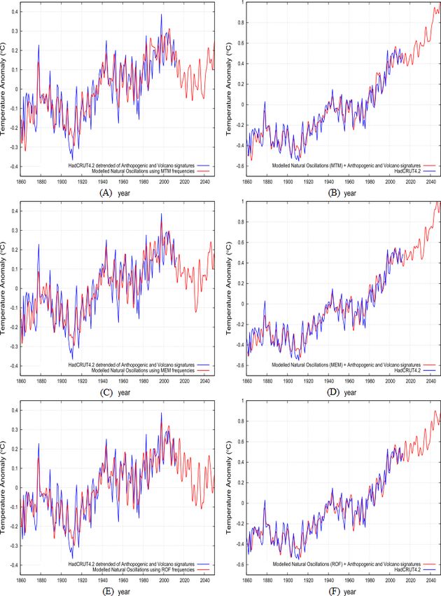
Atmosphere 2021, 12, 147                                                                                            2 of 36

                           approximately capture part of the natural variability of the climate under the condition
                           that the frequencies chosen to represent it have a physical origin. In this regards, it is worth
                           noting that the most accurate and well known geophysical model is the tidal one, where
                           up to 40 harmonics are used to forecast tidal levels at multiple time scales [13].
                                 In contrast, it is observed an absence of internal multidecadal and interdecadal os-
                           cillations in climate model simulations [5,14,15], which likely indicates that the physical
                           origin of most of the observed climatic patterns is still unknown. Yet, if the claimed climatic
                           oscillations are real [16], they cannot be ignored for correctly interpreting climate changes.
                           For example, several studies showed that the Holocene has been characterized by a very
                           large quasi-millennial oscillation [4,17–24]. This large oscillation was responsible for several
                           warm periods such as those that occurred during the Roman and Medieval times [17,21,25].
                           The existence of such a millennial oscillation would have important implications for the
                           correct interpretation of the observed post-industrial global warming [5].
                                 The frequency range from the interannual to the millennial scales during the last
                           century and millennia are particularly important to properly understanding and model-
                           ing the natural climatic variability necessary for validating the climate models and for
                           providing reliable climate projections and forecasts for the near future. In the scientific
                           literature, many relevant climatic oscillations have been hypothesized such as the Atlantic
                           Multidecadal Oscillation, the El Niño Southern Oscillation, the Pacific decadal oscillations,
                           the Interdecadal Pacific Oscillation, the Arctic Oscillation, the North Atlantic Oscillation,
                           the North Pacific Oscillation, and others [26].
                                 The Intergovernmental Panel on Climate Change Fifth Assessment Report [27] ac-
                           knowledges that the natural climatic variability of the climate system is still not understood
                           well and that the Coupled Model Intercomparison Project 5 (CMIP5) global circulation
                           models (GCMs) poorly simulate it. In fact, a mismatch has been observed between the
                           model predictions and the data, such as the temperature standstill observed since 2000 that
                           has been not reproduced by the models predicting warming of about 2 ◦ C/century: see
                           Figure 1 [5,28,29].
                                 A significant mismatch between climate model predictions and data has also been
                           observed throughout the Holocene (during the last 10,000 year) where climate models
                           simulate continuous global warming, mainly in response to rising CO2 and the retreat
                           of ice sheets, while marine and terrestrial proxy records suggest global cooling during
                           the Late Holocene, following the peak warming of the Holocene Thermal Maximum
                           (from about 10,000 to 6000 year ago) [30,31]. Indeed, according to Milanković theory,
                           the Earth’s climate should be approaching the next ice age due to astronomical orbital
                           oscillations [32] although the exact involved physical mechanisms are still unknown.
                           Understanding the climatic changes of the past—e.g., why the last interglacial warm period
                           (130,000–116,000 years before present) was warmer than the Holocene—is still challenging,
                           but improvements are made [33].
                                 Current climate models use radiative forcing (RF) functions as their external in-
                           puts [27]. These functions include a total solar irradiance forcing, a volcano forcing,
                           and several anthropogenic forcing functions deduced from atmospheric concentration vari-
                           ations of greenhouse gases (GHG), aerosol, land-use change, and others ([27], Figure 8.18).
                           The models process them to obtain climatic functions such as local and global surface
                           temperatures. At equilibrium, the global mean surface temperature response ∆T to a
                           radiative forcing variation ∆F is determined by the equation ∆T = λ ∗ ∆F/F2×CO2 , where
                           λ is the equilibrium climate sensitivity (ECS) to radiative forcing. Doubling the CO2 atmo-
                           spheric concentration results in an additional forcing of F2×CO2 = 3.7 W/m2 that should
                           induce about 1 ◦ C warming [34]. In fact, according to the Stefan–Boltzmann law (J = σT 4 ),
                           to increase by 1 ◦ C the temperature of a black-body at a temperature T = 255 K (which
                           would be the mean Earth’s temperature if our planet was a black-body without feedbacks)
                           a radiation increase of ∂J/∂T = 4σT 3 = 3.8 W/m2 K would be needed.
                                 The value of λ is very uncertain because the physics of the main climatic feedbacks (wa-
                           ter vapor and cloud cover) is still poorly understood [35,36]. However, the IPCC AR5 [27]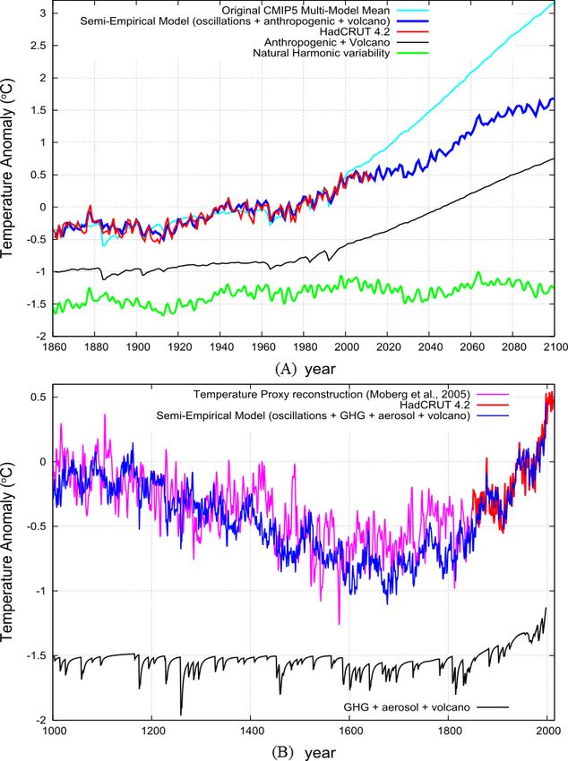
Atmosphere 2021, 12, 147                                                                                                 3 of 36

                           reports that the net feedback should be positive and that the climate sensitivity likely range
                           should be between 1.5 and 4.5 ◦ C for CO2 doubling. In general, it is claimed to be unlikely
                           that the ECS is less than 1 ◦ C or larger than 6 ◦ C [36]. The IPCC ([27], page 745) states
                           the “very high confidence that the primary factor contributing to the spread in equilibrium climate
                           sensitivity continues to be the cloud feedback”.

                           Figure 1. HadCRUT4 global surface temperature (red) (http://www.cru.uea.ac.uk/) [37] from 1850 to
                           2013 against the Coupled Model Intercomparison Project 5 (CMIP5) multi-model mean (blue) of
                           historical plus the average among the RCP4.5, RCP6.0, RCP8.5 scenarios (http://climexp.knmi.nl)
                           from 1861 to 2013. The green area is the 95% (=2σ) temperature confidence of the net (bias + measure-
                           ment + sampling + coverage) error uncertainty. The blue curve is depicted shifted down for visual
                           convenience.

                                The ECS of the CMIP5 models ranges from 2.1 to 4.7 ◦ C, with an average of about
                           3 ◦C  for CO2 doubling, and is very similar to the assessment found in the IPCC AR4
                           (2007) where the CMIP3 models were used ([27], p. 745). Because the climate sensitivity to
                           radiative forcing is not known with sufficient accuracy, if, for example, the real λ were close
                           to 1.5 ◦ C then the CMIP5 models would have on average overestimated the RF warming
                           by a factor of 2; if, on the contrary, λ were close to 4.5 ◦ C then the CMIP5 models would
                           have on average underestimated the RF warming by 50%. Reducing this large uncertainty
                           is necessary for understanding climatic changes [35,36].
                                It has been shown that the CMIP5 models are on average able to approximately
                           reproduce the 0.85 ◦ C warming observed from 1860 to 2000: Figure 1. However, these
                           models do not reproduce any other patterns observed in the historical temperature record
                           with sufficient accuracy [5]. For example, while the standard deviation error of the surface
                           temperature record is about σ = 0.06 ◦ C [37], the root-mean-square deviation (RMSD)
                           values between the temperature signal and the CMIP5 model simulations vary between
                           0.08 and 0.22 ◦ C ([5], Table 2). Thus, the evidence is that there exists a climatic variability
                           that cannot be derived from the adopted RF functions, which are the sole inputs of the
                           current global climate models.
                                Some studies claimed that the natural variability—such as a quasi 60-year and other
                           natural oscillation—is “internal”, that is, it is not externally forced [26,38–40]. Other studies,
                           however, pointed out that this variability can have a solar/astronomical origin [3,5,41–44].
                           Understanding the patterns of natural variability at multiple scales has important con-
                           sequences for a correct evaluation of the climate sensitivity to RF [42,45]. Scafetta [42],
                           Akasofu [46], and Loehle and Scafetta [45] used harmonics and secular trendings to approx-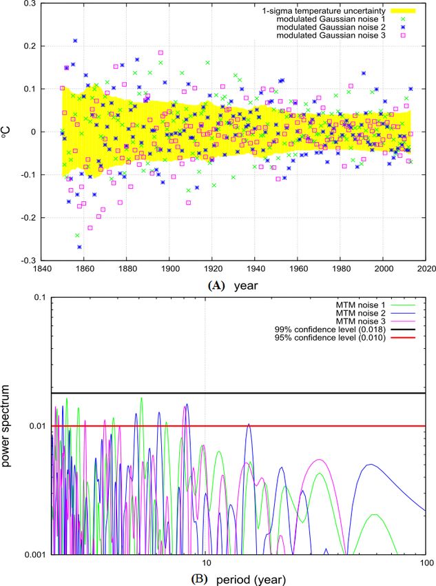
Atmosphere 2021, 12, 147                                                                                            4 of 36

                           imate the multidecadal climatic variability by directly reconstructing the global surface tem-
                           perature patterns with regression models using, as constructors, the available RF functions
                           (e.g., the GHG, aerosol, volcano and solar RFs) plus the Atlantic Multidecadal Oscillation
                           (AMO) record [26,47–49]. The conclusion of the analysis suggested that only about half of
                           the warming observed since 1950 may have anthropogenic causes, while the other half was
                           likely induced by a large quasi 60-year natural oscillation that is particularly evident in
                           several climatic indexes (AMO, PDO, NAO, etc.) for several centuries [26,42,50–58].
                                 If the observed multidecadal climatic variability is natural, the result would imply that
                           low values of ECS likely ∼1.5 ◦ C. The quasi 60-year AMO oscillation was in its warm phase
                           from 1970 to 2000 and should have contributed about half of the observed warming during
                           the same period [42,47,48,51,59]. Other independent studies have concluded that the real
                           climate sensitivity should be between 0.75 to 2.3 ◦ C [5,14,60–67]. In contrast, the CMIP5
                           models predict that nearly 100% of the post-1950 warming was anthropogenic because,
                           according to the same models natural forcing alone (solar + volcano) and internal variability
                           should have induced a net cooling during the same period ([27], FAQ 10.1, Figure 1).
                                 Understanding the solar contribution to climate change is challenging because the so-
                           lar models are uncertain. Moreover, climatic changes may be induced by solar/astronomical
                           forcings alternative to the total solar irradiance (TSI) alone. In fact, according to the GCM
                           simulations, solar forcing could explain only a little fraction (less than 5%) of the warming
                           observed since 1850 [27,40,68,69]. Moreover, the solar models [70] used by the CMIP5
                           GCMs poorly correlate with climatic patterns, while others show a good correlation for
                           several centuries [3,71–75]. For example, the common claim that the AMO, with its warm-
                           ing phase from 1970 to 2000, cannot be related to solar activity is based on the hypothesis
                           that the TSI presents a sightly negative trend during the satellite era, e.g., since 1978 [76].
                           However, such a claim is based on adjusted satellite results [76] that have been always
                           disputed by the original experimental solar scientists responsible for them from 1978 to
                           2014 [77–79] (http://acrim.com/). Using proxy solar model predictions and experimental
                           physical arguments, Scafetta and Willson [80] and Scafetta et al. [81] recently argued that
                           the hypotheses supporting the data modification yielding to the claim that TSI did not
                           increase from 1980 to 2000 are questionable. Therefore, TSI likely increased from 1980 to
                           2000 and slightly decreased after 2000 as the ACRIM and Nimbus7 experimental science
                           teams have always claimed [71,81–83]. Another issue concerns the physical attribution of
                           the 1910–1040 warming and the 1940–1970 cooling periods. During these 60 years, the solar
                           models proposed by Lean [69] and Wang et al. [70] show a steady increase from 1910 to
                           1960 that does not correlate with the observed temperature pattern described above. How-
                           ever, other solar models show that solar activity did peak in the 1940s as the temperature
                           did [3,44,45].
                                 In general, understanding the uncertainty in the solar models is crucial for correctly
                           interpreting the literature. For example, Tung and Zhou [40] claimed that the multidecadal
                           variability shown by the Central England Temperature (CET) record since the 17th century
                           is just an internal variability of the climate system. However, these authors compared the
                           climatic patterns against the solar model proposed by Wang et al. [70] and ignored all other
                           proposed solar models available to date [3,44,72,73,84–86]. Indeed, CET, as well as other
                           climatic records, present a close correlation and spectral coherence from the interannual to
                           the millennial scales with specific solar models [2–5,19,21,23,42,43,71–73,82,83,87–90]: see,
                           for example, Figures 4–6 in Scafetta [73] and Vahrenholt and Lüning [91].
                                 Structural analysis based on regression models of global surface temperature records
                           using as constructors the AMO record plus the RF functions are commonly used to inter-
                           pret climate change attributions [48,49]. However, this methodology cannot identify the
                           physical origin of the natural variability because the AMO record is deduced from the
                           temperature network itself: the AMO is simply defined as the surface temperature of the
                           North Atlantic ocean detrended by its linear warming supposed to be due to anthropogenic
                           warming. Thus, it is not surprising that a regression model of the global surface temper-
                           ature that includes the AMO as a constructor produces a better fit than the RF functions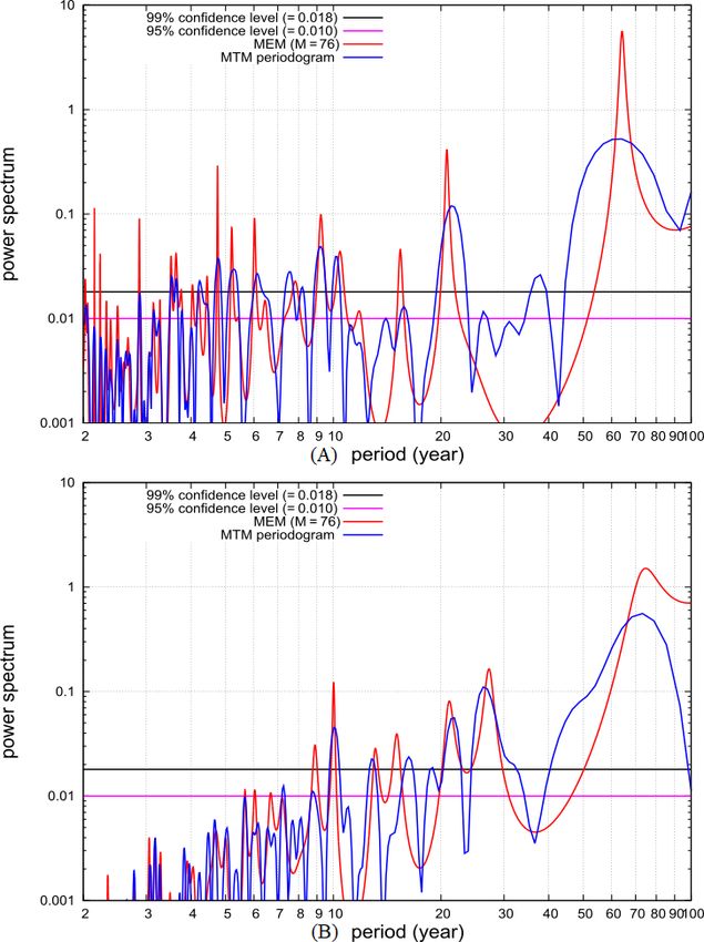
Atmosphere 2021, 12, 147 5 of 36
alone. Instead of demonstrating the physical cause of the multi-decadal climatic variation,
the argument yields a kind of circular reasoning that leaves the real physical attribution
problem unsolved. Some researchers argue that the multidecadal variability, which is
shown in the AMO as well as the other climatic indexes, would fall within the range of the
expected multidecadal variability of the models under specific forcing conditions [92,93],
but the claim is questioned by other authors [5,48,94].
A way to determine whether a climatic pattern—such as the quasi 60-year oscilla-
tion revealed by the AMO index and other climate indexes since 1850 [26]—is an artifact
as claimed in Booth et al. [92] and Mann et al. [93] or a real natural oscillation (it does
not matter whether internal or externally induced), is to consider longer proxy tempera-
ture reconstructions. Indeed, long paleoclimatic records have revealed the existence of a
50–70 year oscillation lasting for centuries and millennia that continues in the AMO os-
cillation observed in the 20th century [42,45,51,54,95–100]. Other climatic oscillations
lasting throughout the Holocene have been found also at periods of about 10 years [101],
20 years [102], 115 years [54,72,103], the DeVries/Suess cycle (~210 years) [85,104], the Eddy
cycle (~1000 years) [2,4,72,105,106], and the Bray–Hallstatt cycle (~2320 years) [84,85]. Simi-
lar oscillations are typically found among proxy records of solar activity [2–4,41,72,85,87,107].
Scafetta [85] has recently demonstrated that all main multidecadal and millennial oscilla-
tions common to both climatic and solar records derive from a restricted set of astronomical
resonances (labeled the invariant inequalities of the solar system) which are made of the
synodic cycles among Jupiter, Saturn, Uranus and Neptune and of their mutual beats.
More specifically, the AMO quasi 60-year pattern, (which is observed for centuries and
millennia [86,97,108]), well fits specific solar proxy models of the last centuries [3,5,43–45].
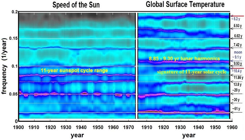
Other climatic oscillations at multiple scales were found among the lunar tidal harmon-
ics [10,109] and the general oscillations of the heliosphere and may regulate solar activ-
ity [42,72,85,110]. It is, therefore, likely that multiple natural oscillations characterize
climate changes.
Herein, I propose that the climate system contains a natural component that is regu-
lated at multiple time scales by harmonics because the moon [10,109], the sun, and other
possible astronomical forcings [41,72,111] should contribute to climate variability harmon-
ically. Scafetta [14,42,112] already showed that a harmonic model of the global surface
temperature (detrended of its secular warming trend) made of four cycles with periods of
9.1, 10.4, 20, and 60 years calibrated in the period 1850–1950 is sufficiently coherent and in
phase with the same model calibrated in the period 1950–2010. To properly reconstruct
and forecast climate changes, the harmonic model needs to be complemented with the
volcano and anthropogenic RF climatic signatures and projections. The anthropogenic
RF climatic signature is non-harmonic and the volcano signature may present some har-
monic recurrence [113] but it is still very intermittent and would be poorly modeled by
sinusoidal harmonics. Thus, the volcano and anthropogenic signatures must be handled
using complementary arguments deduced from the predictions of the climate models.
Regarding the internal climatic variability, it may still present some recurrent patterns
that could be captured by harmonic models as well. Although the observed pattern may
not be all induced by some kind of harmonic astronomical forcing, the system would still
evolve in time-constrained by those forcings and also the internal variability would be
forced to present some kind of recurrence. Among the well-known harmonic astronomical
forcings, it is worth reminding the daily cycle, the annual cycle, multiple tidal cycles, the
orbital oscillations and the solar cycles.
In general, harmonic approximations are expected to approximately simulate climatic
changes. The predicted model trajectory would represent a harmonic ideal limit around
which the actual physical system chaotically fluctuates, as non-linear physics of dynamical
systems predicts (cf: Poincaré’s theory of limit cycles). Moreover, systems made of cou-
pled oscillators can synchronize to their mean internal frequency or to external harmonic
forcings under specific dynamical conditions, as noted first by Huygens in the 17th cen-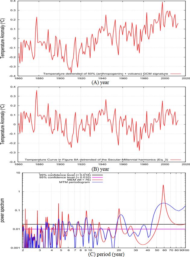
Atmosphere 2021, 12, 147                                                                                             6 of 36

                           tury [42,114,115]. In any case, distinguishing chaos from measurement error in nonlinear
                           systems has always been challenging [116].
                                 In the following, we develop a first approximation harmonic model for reconstructing
                           the natural variability of the global surface temperature record using all statistically relevant
                           oscillations that we could identify both from observations, statistics, and astronomical
                           physical considerations. These oscillations are expected to be numerous.
                                 Sections 2–4 evaluate the confidence levels for spectral analysis of the global surface
                           temperature and propose an empirical model using the found frequencies together with
                           estimated anthropogenic and volcano contributions. The proposed model also includes
                           some secular and millennial climatic harmonics. Section 5 proposes a physical interpreta-
                           tion of the harmonics and develop a harmonic model based on astronomically identified
                           harmonics. To validate our proposed model, we adopt both spectral coherence analyses
                           between different periods. To test the forecast performance of the model for the short
                           timescale, we calibrate it only using the global surface temperature record available in 2013
                           (HadCRUT4.2) and covering the period from 1850 to 2013 [37]. Then, in Section 6 we test
                           its performance by comparing the model prediction against the global surface temperature
                           data available until 2020.

                           2. Evaluation of the Confidence Levels of the Spectral Analysis
                                Figure 1 compares the HadCRUT4.2 global surface temperature annual average record
                           from 1850 to 2013 (http://www.cru.uea.ac.uk/) [37] against the Coupled Model Intercom-
                           parison Project 5 (CMIP5) multi-model mean for the historical plus the RCP4.5, RCP6.0,
                           RCP8.5 (IPCC scenarios of Representative Concentration Pathways) projection experiments
                           from 1861 to 2100 (http://climexp.knmi.nl). The RCP number indicates the projected
                           rising radiative forcing pathway level (in W/m2 ) from 2000 to 2100: RCP 8.5 (rcp85),
                           business-as-usual emission scenario; RCP 6.0 (rcp60), lower emission scenario; RCP 4.5
                           (rcp45), stabilization emission scenario. From 1861 to 2006 the models used the same
                           historical natural and anthropogenic forcings [27]. The blue curve representing the models
                           is depicted on a different anomaly-scale for facilitating a visual comparison finalized to
                           better highlights the pattern differences between the two curves.
                                From 1860 to 2013 a net warming of about 0.85 ± 0.05 ◦ C plus large fluctuations at
                           multiple scales are observed in the HadCRUT4 record. In particular, note the 1850–1880,
                           1910–1940, and 1970–2000 warming periods, the 1880–1910, and 1940–1970 cooling periods,
                           and a temperature standstill since 2000. Figure 1 also shows the 95% (=2σ) confidence
                           interval of the temperature record concerning the estimated (bias + measurement + sam-
                           pling + coverage) error uncertainty (green area).
                                Figure 1 also shows in blue the CMIP5 multi-model mean simulation. While this record
                           approximately reproduces the warming trend from 1861 to 2000, it does not reproduce the
                           oscillations and main patterns observed in the temperature record and fails to predict the
                           temperature standstill observed since 2000. The CMIP5 multi-model mean simulation is
                           very smooth. It is made of a continuous anthropogenic induced warming momentarily
                           interrupted by large volcano eruptions such as Krakatau (1883), Santa Maria (1902), Katmai
                           (1912), Agung (1963), Fuego (1974), El Chichon (1982), Pinatubo (1991), and other minor
                           eruptions ([117], Figure 6).
                                However, the modeled volcano signatures appear often too large and deep relative
                           to the temperature correspondent signals. In addition, the multidecadal patterns are
                           poorly correlated. For example, the 1880–1910 period experienced cooling while the model
                           predicted warming, the period 1910–1940 experienced warming with a trend twice larger
                           than the warming trend predicted by the multi-model mean simulation, the 2000–2014
                           period experienced a temperature standstill while the model predicted steady warming at a
                           rate of about 2 ◦ C/century. For a detailed analysis and comparison between 162 individual
                           CMIP5 general circulation model simulations and the global surface temperature patterns
                           see Scafetta [5].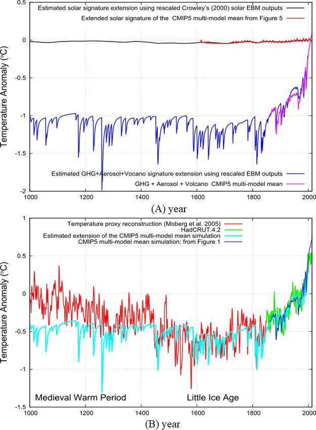
Atmosphere 2021, 12, 147                                                                                                7 of 36

                                The 1σ annual temperature uncertainty function is explicitly shown in Figure 2A.
                           The curve shows that the uncertainty decreases in time and the 1850–2013 average stan-
                           dard deviation is σ ≈ 0.06 ◦ C. Figure 2A also shows three examples of random Gaussian
                           noise records consistent with the temperature uncertainty function. Figure 2B shows their
                           power spectra. The 95% (at about 8.5σ2 /π ≈ 0.010) and 99% (at about 15σ2 /π ≈ 0.018)
                           spectral average confidence levels were calculated using the Multi-Taper Method (MTM)
                           periodogram [118,119]. Using 153-datapoint sequences (from 1861 to 2013) the confidence
                           levels can vary up to about ±15% of the depicted values. In computer simulations us-
                           ing Gaussian records of 153 samples, the MTM periodogram rarely (at most just once)
                           showed spectral peaks exceeding the 99% confidence level (Figure 2B). In the following,
                           the 99% confidence level is used to discriminate the temperature signal oscillations from
                           the background temperature uncertainty.

                           Figure 2. (A) 1σ global surface temperature confidence based on the net bias, measurement, sampling
                           and coverage error uncertainty (yellow area) [37] and three computer-generated Gaussian noise
                           records with a variable standard deviation modulated on the temperature uncertainty. (B) Power
                           spectra of the three computer-generated Gaussian noise records with their 95% and 99% average
                           confidence level using the Multi-Taper Method (MTM) [118,119].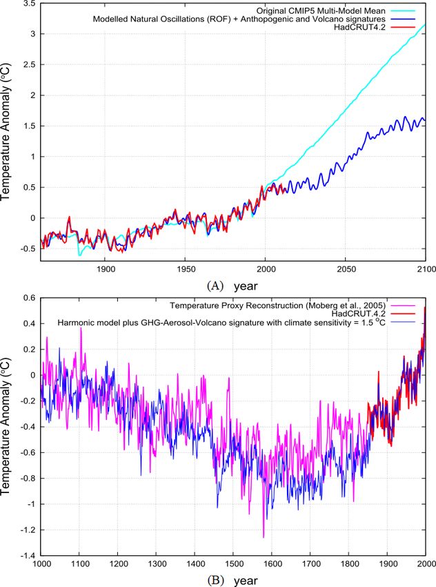
Atmosphere 2021, 12, 147                                                                                         8 of 36

                           3. High-Resolution Spectral Analysis of the Global Surface Temperature Versus the
                           CMIP5 Multi-Model Mean Function
                                Figure 3A compares the power spectra of the global surface temperature record and
                           Figure 3B shows the same for the CMIP5 multi-model mean function using 153-year data
                           from 1861 to 2013. The power spectra are calculated using MTM and the Maximum
                           Entropy Method (MEM) with the SSA-MTM toolkit for spectral analysis [118,119]. The two
                           methodologies are used to better identify spurious spectral peaks. For example, the MTM
                           spectral peak at about 40 years is not confirmed by MEM and, therefore, is excluded from
                           the harmonic modeling made below.
                                The two power spectra depicted in Figure 3A,B are quite different from each other.
                           The global surface temperature record presents significant spectral peaks (at the 99% confi-
                           dence level) at multiple time scales, from 2 to 100 year periods (see Table 1). The CMIP5
                           multi-model mean function does not present any significant spectral peak for periods
                           shorter than 10 years. For periods larger than 10 years the temperature record and the
                           CMIP5 multi-model mean function present substantially different spectral peaks. For ex-
                           ample, the temperature presents a large spectral peak at the about 60-year period that
                           corresponds to an evident oscillation [5,108]. Yet, the model presents a spectral peak at
                           about 70–80 year period.
                                The 70–80 year recurrence found in the CMIP5 multi-model mean function is not a
                           real dynamical oscillation because it is due to the timing of the major volcano eruptions
                           that occurred in the 20th century, which are separated by about 70–80 years. There exists
                           a similarity between the volcano sequences that occurred 1880–1920 and in 1960–2000
                           (Figure 1) [14]. Only a common spectral peak at about 10 and 20 years between the temper-
                           ature and the model power spectra are observed, although with different spectral power.
                           These correspondences occurs because the CMIP5 multi-model mean function includes a
                           small signature from the 11-year (and 22-year) total solar irradiance solar cycle. However,
                           in the climate models, a quasi 10-year and 20-year spectral peaks could also derive from
                           the timing of volcano eruptions, because during the 1880–1920 and 1960–2000 periods
                           they occur in intervals of about 10 and 20 years, respectively (Figure 1). Compare against
                           (Scafetta [14], Figures 1 and 2) where it was shown that typical model simulations do not
                           present a realistic harmonic pattern at the 10-, 20-, and 60-year periodicities. However,
                           an analysis of 600-year long volcano indexes highlighted the presence of quasi 10-, 33-,
                           and 88-year recurrence [113].
                                Because the power spectra of the temperature signal present multiple spectral peaks at
                           the 99% and above confidence level, the patterns described by these spectral peaks must be
                           considered real climatic patterns and not just random fluctuations. Thus, climate models
                           should reproduce those patterns. If they do not, as it has been already demonstrated [5],
                           then the evidence is that the models are missing mechanisms necessary for reconstructing
                           the dynamics of the climate system.
                                The individual model simulations do show a rich fluctuating variability at all time
                           scales: see Figures 4–11 in Scafetta [5]. However, these fluctuations appear to be red-noise
                           dynamical fluctuations with no resemblance to the real temperature variability [5,14]. The
                           model’s inability to systematically reproduce the real temperature fluctuations and/or
                           oscillations is the reason why when the individual model simulations are averaged into a
                           CMIP5 multi-model ensemble mean function, the latter looks very smooth. The CMIP5
                           multi-model mean function represents the common patterns reconstructed by the CMIP5
                           models, which is what these models, in their ensemble, predict. In fact, even if the global
                           surface temperature signal may be correlated with a model simulation better than with
                           another one [5], if the good fit is not consistent among the simulations, chances are that
                           the result is a coincidence. Indeed, also random noise generators may produce specific
                           sequences that can well fit a given physical sequence.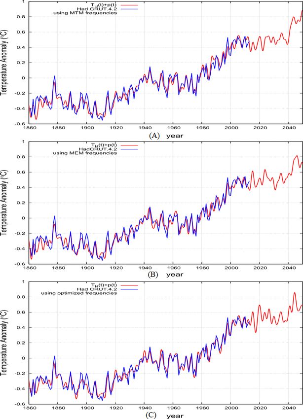
Atmosphere 2021, 12, 147                                                                                             9 of 36

                           Figure 3. Power spectra of the global surface temperature record (A) and the CMIP5 multi-model
                           mean function (B). The power spectra are calculated using the Multi-Taper Method (MTM) and the
                           Maximum Entropy Method (MEM) using the SSA-MTM toolkit for spectral analysis [118,119]. The
                           95% and 99% confidence levels are deduced from the analysis of the theoretical temperature error
                           analyzed in Figure 2.

                                Table 1 reports the 13 frequencies obtained from the MTM spectral peaks that are above
                           the 99% confidence level, the same frequencies evaluated by MEM, and those obtained
                           using a regression harmonic model. The amplitudes and phases of the harmonics are
                           calculated using the following temperature regression equation

                                                  TH (t) = Z + ∑ Ai sin(2π (Ωi (t − 2000) + φ)),                        (1)
                                                                 i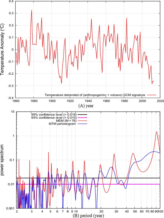
Atmosphere 2021, 12, 147                                                                                                        10 of 36

                                  which has been applied to the temperature record after it was detrended of its quadratic
                                  fit function
                                                                 p(t) = a ∗ (t − 1850)2 + b                            (2)
                                  with a = 0.0000308 ± 0.000002 and b = −0.395 ± 0.02. In Equation (1), Z = −0.0137 when
                                  the MTM frequencies are used, Z = −0.0113 when the MEM frequencies are used and
                                  Z = −0.0109 when the optimized frequencies are used.

      Table 1. Regression coefficient of Equation (1) using the temperature MTM and MEM spectral peaks with a 99% con-
      fidence level depicted in Figure 3A and after a regression optimization of the frequencies. For a 153-year long se-
      quence the spectral resolution is dΩ = 1/153 = 0.0065 yr−1 and the statistical error in the reported frequencies is
      ∇Ω = ±0.5 dΩ = ±0.003 yr−1 . The three sets of frequencies are compatible within their statistical error. Ω−1 is the period,
      Ω is the frequency, A is the amplitude of the sine wave and φ is the phase.

    MTM Spectral Peak Frequencies               MEM Spectral Peak Frequencies              Regression Optimized Frequencies
  Ω−1 (yr)       Ω (yr−1 )   A (◦ C)    φ      Ω−1 (yr)     Ω (yr−1 )    A (◦ C)     φ     Ω−1 (yr)     Ω (yr−1 )    A (◦ C)     φ
    62.11         0.0161     0.118     0.20      64.10       0.0156       0.122     0.16     65.79        0.0152      0.121     0.14
    21.33         0.0469     0.042     1.00      20.75       0.0482       0.044     0.08     20.70        0.0483      0.046     0.10
    10.24         0.0977     0.027     0.13      10.44       0.0958       0.025     0.97     10.21        0.0979      0.031     0.13
    9.225         0.1084     0.038     0.45      9.234       0.1083       0.041     0.44     9.183        0.1089      0.039     0.50
    8.190         0.1221     0.024     0.82                                                  8.190        0.1221      0.021     0.80
                                                 7.831       0.1277       0.015     0.38
    7.530         0.1328     0.024     0.66                                                  7.645        0.1308      0.024     0.57
    6.131         0.1631     0.021     0.27      6.020       0.1661       0.027     0.61     6.254        0.1599      0.027     0.94
    5.277         0.1895     0.025     0.33      5.200       0.1923       0.025     0.49     5.236        0.1910      0.029     0.42
    4.762         0.2100     0.031     0.04      4.746       0.2107       0.033     0.10     4.773        0.2095      0.034     0.01
    4.232         0.2363     0.017     0.46      4.202       0.2380       0.022     0.58     4.179        0.2393      0.026     0.65
    3.644         0.2744     0.025     0.70      3.635       0.2751       0.024     0.73     3.628        0.2756      0.029     0.79
    3.531         0.2832     0.023     0.89      3.516       0.2844       0.021     0.95     3.556        0.2812      0.028     0.79
    2.876         0.3477     0.025     0.95      2.869       0.3486       0.025     0.02     2.875        0.3478      0.025     0.97

                                       Figure 4 shows the global surface temperature against the regression model made
                                  of Equation (1) + Equation (2). The model well reconstructs the temperature fluctuations.
                                  The root mean square of the residuals (rmsr) is rmsr ≈ 0.069 ◦ C when the MTM spectral
                                  peak frequencies are used; rmsr ≈ 0.068 ◦ C when the MEM spectral peak frequencies
                                  are used; and rmsr ≈ 0.061 ◦ C when the regression optimized frequencies are used. See
                                  Table 1. These rmsr values are compatible with the temperature experimental uncertainty
                                  shown in Figure 2. The model predicts a continued temperature standstill until 2030–2040.
                                  Because of the rapid oscillations, the temperature should experience a local maximum
                                  during 2015, followed by a local minimum during 2017 and another local maximum in 2020.
                                  However, for the period 2015–2020 the optimized frequency model (Figure 4C) predicts
                                  a larger oscillation than the MTM frequency model (Figure 4A); the model based on the
                                  MEM frequencies is approximately between the other two simulations. All three model
                                  predictions for the period 2014–2050 are quite similar to each other in predicting the timing
                                  of the major temperature peaks although with slightly different amplitudes.
Atmosphere 2021, 12, 147 11 of 36
Figure 4. The global surface temperature (blue) against the regression model made of Equation (1) +
Equation (2) (red) using: (A) The MTM spectral peak frequencies (rmsr ≈ 0.069 ◦ C); (B) the MEM
spectral peak frequencies (rmsr ≈ 0.068 ◦ C); (C) the regression optimized frequencies are used
(rmsr ≈ 0.061 ◦ C) . See Table 1.
4. Optimized Spectral Analysis and Harmonic Modeling
In this section, we propose a methodology to optimize our analysis of the global
surface temperature record. The harmonic analysis made in the previous section could be
biased, in particular at the lower frequencies.
The temperature record combines a harmonic component (possibly induced by solar,
astronomical, and lunar oscillations plus additional independent internal oscillations with
a non-harmonic component such as that induced by the anthropogenic (GHG, aerosol,
etc.) and volcano forcing components that cannot be captured by a simple quadratic
fit of Equation (2). On large scales, the volcano signature may present some harmonic
components [113], but because such a signature is intermittent and quite sporadic, in a short
record such as the global surface temperature since 1850 it is better to keep it separated
from the harmonic dynamical component. Thus, the harmonic analysis could be optimizedAtmosphere 2021, 12, 147 12 of 36
by applying it to a temperature signal detrended of the theoretical signature made by the
anthropogenic plus volcano forcings.
In the following, two independent cases are analyzed: (1) the non-harmonic temper-
ature component is assumed to be simulated by the CMIP5 multi-model mean function
depicted in Figure 1 minus an estimate of the small modeled temperature signature due to
the total solar irradiance forcing; (2) the non-harmonic temperature component is assumed
to be simulated by 50% of the CMIP5 multi-model mean function depicted in Figure 1
minus an estimate of the small model temperature signature of the total solar irradiance
forcing, as proposed in References [5,67]. The CMIP5 multi-model mean function is used
because it may be a reasonable estimate of the temperature signature of the RF functions.
There is a need of removing the solar signature from the CMIP5 multi-model mean
function because (1) such a signature contains a 10–12 year harmonic that is part of the
astronomical harmonics of the system that need to be modeled by the harmonic model,
and (2) the low-frequency component of the solar forcing function used by the CMIP5
models may be wrong [5,80]. This is done in Figure 5 that shows a reconstruction of the
solar average signature at the surface as typically modeled by general circulation models,
which is extremely small [27]. This solar average signature was made rescaling the total
solar irradiance record by Wang et al. [70], which was used by the CMIP5 as the solar input
of the models, on the global mean solar signature at the surface produced by the GISS
ModelE from 1945 to 2003 [68,120]. Note that the GISS ModelE simulations were made in
2003 and used a precedent solar model that agrees with that proposed by Wang et al. [70]
only since 1945.
The solar signature is detrended from the CMIP5 multi-model mean simulation to
obtain an estimate of the global surface temperature signature of the anthropogenic plus
volcano forcings according to the following formula:
CMIP5anthr&volca (t) = CMIP5(t) − CMIP5solar (t). (3)
This corrected function is the purple curve in Figure 5 and is used below as the
CMIP5 multi-model mean simulation for the anthropogenic plus volcano global surface
temperature signature.
Figure 5. (Black) solar signature at the surface reproduced by the GISS ModelE from 1945 to
2003 [68,120]. (Red) reconstruction of the solar signature modeled by the global circulation models
(GCMs) using the total solar irradiance record by Wang et al. [70]. (Blue) CMIP5 multi-model mean
simulation (from Figure 1). (Purple) Coupled Model Intercomparison Project 5 (CMIP5) multi-model
mean simulation detrended of the solar signature, Equation (3).Atmosphere 2021, 12, 147 13 of 36
4.1. The Non-Harmonic Temperature Component is Assumed to be Simulated by the
Anthropogenic + Volcano CMIP5 Multi-Model Mean Temperature Function
Figure 6A shows the temperature residual after the function CMIP5anthr&volca (t) (pur-
ple curve in Figure 5) is detrended from the temperature data (T (t)) according to the
following formula:
Tresidual (t) = T (t) − CMIP5anthr&volca (t). (4)
Figure 6B shows its power spectra. The spectral peaks at periods shorter than 20 years
are similar to those found in Figure 3A. However, for larger timescales, uncertain spectral
patterns are observed: MEM and MTM provide significantly different patterns.
A simple visual analysis of the residual depicted in Figure 6A indicates that the CMIP5
multi-model signature fails to reconstruct the temperature signature at both sub-decadal
and multidecadal scales. In fact, large multidecadal biases with an amplitude up to 0.3 ◦ C
lasting up to 30–40 years are observed. Knight et al. [121] observed that: “Near-zero and
even negative trends are common for intervals of a decade or less in the simulations, due
to the model’s internal climate variability. The simulations rule out (at the 95% level) zero
trends for intervals of 15 year or more, suggesting that an observed absence of warming of
this duration is needed to create a discrepancy with the expected present-day warming
rate.” Indeed, the large biases observed in Figure 6A last for more than 15 years. Thus,
the result suggests that major physical flaws exist in the CMIP5 GCMs. This casts doubts
on the ability of the CMIP5 models to properly interpret and project the global surface
temperature both at the sub-decadal scale and the multidecadal and secular scales, as noted
by numerous researchers [14,26,42,47–49,58,122].
It is simple to demonstrate that the CMIP5 general circulation models miss impor-
tant physical mechanisms responsible not only for the high-frequency component of the
temperature dynamics such as the El Niño–Southern Oscillation (ENSO) signal but also
for the low-frequency component at the multidecadal to millennial timescales. For the
multidecadal scales, it is possible to test their ability in reproducing the 60-year temperature
oscillation that is commonly found in the Atlantic Multidecadal Oscillation, which the
CMIP5 GCMs are not able to reproduce [14,47–49,122].
For the secular and millennial timescale, it is possible to check how well the CMIP5
models would perform in reconstructing the temperature variation during the last mil-
lennium by empirically extending them back in time since the CMIP5 simulations start
in 1861.
Multiple recent paleoclimatic temperature reconstructions are available and present a
marked millennial cycle made of a Medieval Warm Period (MWP 900–1400) followed by a
Little Ice Age (LIA 1450–1800) and finally by a Modern Warm Period (since
1900) [17,19–21,23,105,123,124].
To test how well this pattern would agree with the physics implemented in the CMIP5
models, their mean ensemble function needs to be empirically extended back in time using
the known climatic forcings for the last millennium. This can be done by rescaling the
outputs of typical energy balance models that have been forced with solar, GHG, aerosol,
and volcano forcings on the CMIP5 multi-model mean forcing signatures so that the latter
could be extended by the former for 1000 years. I will use the energy balance model outputs
of (Crowley [125], Figure 3), with an appropriate rescaling.Atmosphere 2021, 12, 147 14 of 36
Figure 6. (A) HadCRUT4 detrended of the CMIP5 multi-model mean simulation relative to anthro-
pogenic and volcanic forcings alone (blue curve in Figure 5), Equation (4). (B) Power MTM and MEM
spectra of the record depicted in (A).
Figure 7A shows in black an extension of the estimated solar signature of the CMIP5
multi-model mean shown in Figure 5. It is made by extending the solar temperature
signature derived from Wang et al. [70] (shown in red in Figure 5) with the average solar
output function deduced from the energy balance model proposed by (Crowley [125],
Figure 3) after an appropriate rescaling. It would be expected that the solar signature
continues to be very small during the entire millennium because it already was small from
1860 to 2013.
The figure also shows in blue the estimated GHG-Aerosol-Volcano signature extension
of the CMIP5 multi-model mean correspondent signature (purple curve in Figure 6).
The optimal rescaling required a factor of 1.5 because the energy balance model used by
Crowley [125], whose outputs are herein used to make the extensions, used an equilibrium
climate sensitivity of 2.0 ◦ C for CO2 doubling while the CMIP5 have an average climateAtmosphere 2021, 12, 147 15 of 36
sensitivity of 3.0 ◦ C [27]. The same scaling could not be applied for the solar signature
because Crowley [125] used solar records with a larger secular and millennial variability
than the Wang et al. [70]’s solar record used by the CMIP5 records. Thus, for the solar
signature, it was necessary to apply an appropriate empirical rescaling, as shown in
Figure 7A.
Figure 7B shows in blue the estimated extension of the CMIP5 multi-model mean
function, Ex.CMIP5(t), which is made of the solar plus the GHG+Aerosol+Volcano (blue
and purple) signature extensions depicted in Figure 7A according to the following formula:
Ex.CMIP5(t) = Ex.CMIP5anthr&volca (t) + Ex.CMIP5solar (t). (5)
This model is compared against a typical modern reconstruction of the northern hemi-
sphere temperature [124] substituted since 1850 by the instrumental temperature record.
Figure 7B shows that the model performs relatively well in reconstructing the tem-
perature warming after 1500, that is since the Little Ice Age. The result agrees with the
independent analysis of Lovejoy [126] that analyzed paleoclimatic temperature records
since 1500 and found that the warming observed since 1500 could be approximately inter-
preted by climate models using an ECS of about 3 ◦ C for CO2 doubling, as modeled on
average by the CMIP5 GCMs.
However, as Figure 7B also shows, before 1500 the extended CMIP5 model progres-
sively diverges from the temperature signal. In 1000 AD the divergence between the model
and the data becomes as large as 0.5 ◦ C, which is about 50% of the warming observed from
1800 to 2000.
Therefore, the CMIP5 models are physically compatible only with pre-industrial global
surface temperature records that show a small variability on the multidecadal-secular-
millennial time scales (about 0.2 ◦ C) and that on shorter time scales could at most present
spikes induced by the volcano eruptions. According to this scenario, the post-1850 warming
of about 0.85 ◦ C had to be interpreted as historically anomalous. Moreover, Figure 7A
clearly shows that solar variability does not contribute significantly to climate changes.
This picture well fits the so-called Hockey-Stick temperature reconstructions that were
quite popular in 1998–2005 [125,127,128] that claimed that the preindustrial temperature
varied little (about 0.2–0.3 ◦ C) and those well-known phenomena such MWP and LIA only
occurred in limited regions of the Earth (e.g., in Europe).
However, as Figure 7B shows, modern reconstructions of the past climate have ev-
idenced the existence of a far larger climatic variability on the secular-millennial time
scales [123,124]. Modern multi-proxy temperature reconstructions of the extra-tropical
northern hemisphere during the last two millennia even claim that the MWP experi-
enced periods as warm as the actual period [17,19,21,23,105], which well fits strong his-
torical inferences [129]. Even ignoring the evidence from the extra-tropical northern
hemisphere, Figure 7B indicates that the CMIP5 models would severely fail to repro-
duce the large pre-industrial warming periods such as the MWP predicted by modern
paleoclimatic temperature reconstructions. The same failure in reconstructing the Me-
dieval Warm Period around 1000 AD could be observed also by comparing an ensem-
ble of recent reconstructions of the north hemisphere temperature reconstruction and
the last millennium climate model simulations ([27], data and graphs are available at
https://www.ncdc.noaa.gov/global-warming/last-1000-years and at https://www.ipcc.
ch/report/ar5/wg1/technical-summary/wgi_ar5_tsfig_ch5_v2-1-5/) [130].Atmosphere 2021, 12, 147 16 of 36
Figure 7. (A) Extension of the CMIP5 multi-model mean simulation referring to the solar signa-
ture (red and black) and the greenhouse gas (GHG)+Aerosol+Volcano (blue and purple) signature.
The extensions are constructed by calibrating the correspondent energy balance model outputs of
(Crowley [125], Figure 3)on the CMIP5 multi-model mean estimates. (B) Comparison between the
extended CMIP5 multi-model mean simulation (cyan) made by summing the black and blue curved
in A Equation (5) against the temperature proxy reconstruction by Moberg et al. [124] (red) calibrated
and extended with the HadCRUT record (green) since 1850.
Indeed, recent studies have shown that to properly reconstruct the MWP and the
cooling from it to the LIA, a far greater solar signature on the climate system than what
modeled by the CMIP5 models would be required [3,5,67,131,132]. In general, the claim that
solar variability contributes very little to climate change is contradicted by very numerous
studies [2–4,72,87,90,133]. These results imply that either the CMIP5 models are using
wrong solar irradiance forcings [3,80] or that they are missing alternative solar-climate
related mechanisms such as a cloud modulation from cosmic rays and others [5,6,8,85–87].Atmosphere 2021, 12, 147 17 of 36
Because paleoclimatic temperature proxy models reveal that the Holocene temperature
is characterized by a quasi-millennial large oscillation that well fits an equivalent oscillation
found in the solar/heliospheric proxy models [2,4,17,72,105,134], the evidence is that
the CMIP5 models miss important mechanisms with a likely solar-astronomical origin.
These may be responsible for many climatic oscillations missed by the CMIP5 models.
The millennial oscillation has been quite persistent during the Holocene [2,4,21,72] giving
origin to periods such as the Roman Maximum (around 2000 years ago), the Dark Age
Period (400–800 AD), the Medieval Warm Period (800–1400 AD), and the Little Ice Age
(1400–1850) [17,19,105]. Finally, the 21st century should be characterized by a millennial
temperature maximum. Thus, using the temperature reconstruction by Moberg et al. [124]
(which can be considered intermediate among those that show a smaller and a larger
variability) Figure 7B suggests that the large millennial natural oscillation could have
contributed at least about 50% of the warming observed since 1850 [5,72,134].
4.2. The Non-Harmonic Temperature Component is Assumed to be Simulated by 50% of the
Anthropogenic + Volcano CMIP5 Multi-Model Mean Temperature Function
The above result implies that the real climate sensitivity to CO2 doubling could
be about half of the 3 ◦ C modeled by the CMIP5 models [27]. Indeed, an ECS value
equal to about 1.5 ◦ C (or at least between 1 and 2 ◦ C) is consistent with several modern
studies [14,47,48,60–66]. If the real climate sensitivity is about half of what predicted by
the CMIP5 models, then the real temperature signature of the radiative forcings used in the
CMIP5 models should be about half than what these models have simulated. Thus, in first
approximation, the temperature residual that would capture the hypothesized harmonic
component of the climate system would be given by [5,67]:
TH.residual (t) = T (t) − 0.5 · CMIP5anthr&volca (t). (6)
Figure 8A shows the global surface temperature detrended of the anthropogenic plus
volcano CMIP5 multi-model mean temperature function attenuated by half. This record
represents the residual natural variability according to the Equation (6). The signal shows
an upward warming trend and an evident quasi 60-year oscillation plus faster oscillations.
According to our hypothesis, these patterns are produced by physical mechanisms regulat-
ing the climate from the sub-decadal to the millennial timescale, which are not simulated
by the CMIP5 models. A first result is that natural factors would have been responsible for
about 0.5 ◦ C warming observed since 1910.
The temperature residual depicted in Figure 8A shows a slightly asymmetric 60-year
oscillation. The 60-year oscillation from 1880 to 1940 is slightly larger than the oscillation
from 1940 to 2000. Scafetta [5,72] argued that the observed warming and the 60-year cycle
asymmetry could be due to two solar/astronomical major long oscillations: (1) a millennial
oscillation; (2) a quasi 115-year oscillation that characterizes the 100–130 year pace-time
between the grand solar minima such as the Maunder Minimum (1645–7015) and the
Dalton Minimum (1790 to 1830) [54]. For astronomical reasons [72], the 115-year oscillation
should have had a minimum in 1922 and should have peaked in 1980 causing an apparent
asymmetry in the amplitude of the 60-year oscillation. Scafetta [5] modeled these two long
oscillations with the following equation:
h i
Hsec&mil (t) = Bm H (1680 − t) cos 2π t−1206 1077
+ H (t − 1680) cos 2π t−760
2060
(7)
+ Bs cos 2π t−115
1980
,
where the millennial amplitude, Bm = 0.35, and the secular amplitude, Bs = 0.05, were
approximately deduced from the paleoclimatic temperature records such as those proposed
by Moberg et al. [124], Mann et al. [123], and Ljungqvist [17], and the Heaviside step
function H ( x ) is equal to 1 for x > 0 and to 0 for x < 0. Note that the millennial
temperature oscillation, which was theoretically estimated to be 983 years Scafetta [72],Atmosphere 2021, 12, 147 18 of 36
is skewed having theoretical maxima in 1077 and 2060 (which were determined from
astronomical considerations), and a minimum in 1680 during the Maunder solar grand
minimum. This is why Equation (7) could represent the millennial oscillation using two
truncated harmonics: note that 1206/2 + 760/2 = 983. The skewness is likely induced
by additional multi-secular oscillations that are ignored here [2]. The reported equation
is valid only within the interval 1077–2060 because it describes only one temperature
millennial cycle. Figure 8B shows the sub-secular temperature variability TH.residual.subsec (t)
obtained by detrending the record depicted in Figure 8A Equation (6) of the secular and
millennial component Equation (7) according to the formula:
TH.residual.subsec (t) = TH.residual (t) − Hsec&mil (t). (8)
Figure 8B shows that this residual is regulated by a nearly stationary quasi 60-year
oscillation. Figure 8C shows the MTM and MEM spectra of the detrended record depicted
in Figure 8A. The major spectral peaks are listed in Table 2. The power spectrum functions
shown in Figure 8C are quite similar to those observed in Figure 3A. However, a few
important details emerge. For example, looking at the MEM results, which are likely
more precise, the following results are found: (1) the quasi 60-year spectral peak moved
from 64.1 years to 58.8 years, which is closer to the 60-year periodicity that represents a
theoretical astronomical/heliospheric harmonic and is confirmed by several paleoclimatic
evidences [51,54,85,86,98,99]; (2) the quasi 20-year spectral peak moved from 20.7 years
to 20.3 years which is closer to the 20-year periodicity that also represents a major the-
oretical astronomical/heliospheric harmonic [42,72] and is confirmed by paleoclimatic
records [102]; the spectral peak at 10.4 years moved to 10.7 years, which is closer to the aver-
age solar cycle length since 1860 which was about 10.8 years Scafetta [72]; the spectral peak
at 9.2 years moved to 9.3 years, which better corresponds to the first harmonic of the 18.6 lu-
nar nodal cycle and further confirms the lunar origin of this oscillation [10,42,135]. In any
case, the frequency values evaluated with the various methodologies are slightly different
but still consistent with each other within the spectral resolution of the analysis that for a
153-year long record implies a frequency error of ∇Ω = ±0.5/153 = ±0.0033 yr −1 . Table 2
reports the frequencies at the 99% confidence level relative to the MTM and MEM spectra
with their amplitude and phase. Table 2 also reports a harmonic regression optimization of
the various parameters using Equation (1).
The full semi-empirical climate model is made by summing the harmonic components
plus the anthropogenic and volcano ones, that is
T (t) = Z + ∑ Ai sin(2π (Ωi (t − 2000) + φ)) + Hsec&mil (t) + 0.5 · CMIP5anthr&volca (t) (9)
i
where the harmonic coefficients are reported in Table 2. The first two rows of Table 2
report the coefficients of the millennial and secular theoretical oscillations expressed in
the sinus formalism of Equation (9). Figure 9 depicts Equation (9) against the temperature
signal. The left panels of Figure 9 show only the natural harmonic variability and the
models forecast a natural cooling until 2030–2040. This cooling should compensate for the
projected anthropogenic warming so that the temperature remains steady until 2030–2040.
Faster oscillations are observed and the models predict that the next local temperature
maxima should occur in 2015 and 2020.You can also read


