Integrated modeling of canopy photosynthesis, fluorescence, and the transfer of energy, mass, and momentum in the soil-plant-atmosphere continuum ...
←
→
Page content transcription
If your browser does not render page correctly, please read the page content below
Geosci. Model Dev., 14, 1379–1407, 2021
https://doi.org/10.5194/gmd-14-1379-2021
© Author(s) 2021. This work is distributed under
the Creative Commons Attribution 4.0 License.

Integrated modeling of canopy photosynthesis, fluorescence,
and the transfer of energy, mass, and momentum in
the soil–plant–atmosphere continuum
(STEMMUS–SCOPE v1.0.0)
Yunfei Wang1,2,3,5 , Yijian Zeng3 , Lianyu Yu3 , Peiqi Yang3 , Christiaan Van der Tol3 , Qiang Yu5 , Xiaoliang Lü5 ,
Huanjie Cai1,2 , and Zhongbo Su3,4
1 College of Water Resources and Architectural Engineering, Northwest Agriculture and Forestry University, Yangling, China
2 Instituteof Water Saving Agriculture in Arid Regions of China (IWSA), Northwest Agriculture and Forestry University,
Yangling, China
3 Faculty of Geo-Information Science and Earth Observation, University of Twente, Enschede, the Netherlands
4 Key Laboratory of Subsurface Hydrology and Ecological Effects in Arid Region, Ministry of Education,

School of Water and Environment, Chang’an University, Xi’an, China
5 State Key Laboratory of Soil Erosion and Dryland Farming on the Loess Plateau, Institute of Water and Soil Conservation,

Northwest Agriculture and Forestry University, Yangling, China

Correspondence: Huanjie Cai (huanjiec@yahoo.com) and Zhongbo Su (z.su@utwente.nl)

Received: 31 March 2020 – Discussion started: 2 June 2020
Revised: 17 January 2021 – Accepted: 20 January 2021 – Published: 11 March 2021

Abstract. Root water uptake by plants is a vital process that    1   Introduction
influences terrestrial energy, water, and carbon exchanges.
At the soil, vegetation, and atmosphere interfaces, root wa-
ter uptake and solar radiation predominantly regulate the dy-    Root water uptake (RWU) by plants is a critical process con-
namics and health of vegetation growth, which can be re-         trolling water and energy exchanges between the land sur-
motely monitored by satellites, using the soil–plant relation-   face and the atmosphere and, as a result, plant growth. The
ship proxy – solar-induced chlorophyll fluorescence. How-        representation of RWU is an essential component of eco-
ever, most current canopy photosynthesis and fluorescence        hydrological models that simulate terrestrial water, energy,
models do not account for root water uptake, which compro-       and carbon fluxes (Seneviratne et al., 2010; Wang and Smith,
mises their applications under water-stressed conditions. To     2004). However, most of these models consider the above-
address this limitation, this study integrated photosynthesis,   ground processes in much greater detail than belowground
fluorescence emission, and transfer of energy, mass, and mo-     processes; therefore, they have a limited ability to repre-
mentum in the soil–plant–atmosphere continuum system, via        sent the dynamic response of plant water uptake to water
a simplified 1D root growth model and a resistance scheme        stress. A particular mechanism of importance for plants to
linking soil, roots, leaves, and the atmosphere. The coupled     mitigate water stress is the compensatory root water uptake
model was evaluated with field measurements of maize and         (CRWU) which refers to the process by which water uptake
grass canopies. The results indicated that the simulation of     from sparsely rooted but well-watered parts of the root zone
land surface fluxes was significantly improved by the cou-       compensates for stress in other parts (Jarvis, 2011). The fail-
pled model, especially when the canopy experienced mod-          ure to account for compensatory water uptake and the asso-
erate water stress. This finding highlights the importance of    ciated hydraulic lift from deep subsoil (Caldwell et al., 1998;
enhanced soil heat and moisture transfer, as well as dynamic     Espeleta et al., 2004; Amenu and Kumar, 2007; Fu et al.,
root growth, on simulating ecosystem functioning.                2016) can lead to significant uncertainties in simulating the

Published by Copernicus Publications on behalf of the European Geosciences Union.
1380                             Y. Wang et al.: Integrated modeling of processes in the soil–plant–atmosphere continuum

plant growth and corresponding ecohydrological processes            As such, there is no explicit parametrization of the effects of
(Seneviratne et al., 2010).                                         soil moisture variations on the photosynthetic or stomatal pa-
   Because the spatial (i.e., 1D vertical) pattern of RWU is        rameters. Consequently, soil moisture effects are only “visi-
determined by the spatial distribution of the root system,          ble” in SCOPE if the lack of soil moisture affects the optical
knowledge of the latter is essential for predicting the spatial     or thermal remote sensing signals (i.e., during water stress
distribution of water contents and water fluxes in soils. The       periods). The lack of such a link between soil moisture avail-
distribution of roots and their growth are, in turn, sensitive to   ability and remote sensing signals compromises the capacity
various physical, chemical, and biological factors, as well as      of SCOPE to simulate and predict drought events on vegeta-
to soil hydraulic properties that influence the availability of     tion functioning.
water for plants (Beaudoin et al., 2009). Many attempts have           The change in vegetation optical appearance as a result
been made in the past to develop root growth models that ac-        of soil moisture variations can only partially explain the
count for the influence of various environmental factors such       soil moisture effect on ecosystem functioning (Bayat et al.,
as temperature, aeration, soil water availability, and soil com-    2018), which leads to considerably biased estimations of
paction. Existing root growth models range from complex,            the gross primary productivity (GPP) and evapotranspira-
3D root architecture models (Bingham and Wu, 2011; Leit-            tion (ET) under water-limited conditions. This presents a
ner et al., 2010; Wu et al., 2005) to much simpler root growth      challenge with respect to using SCOPE for ecosystems in
models that are implemented within more complex models              arid and semiarid areas, where water availability is the pri-
such as EPIC (Williams et al., 1989) and DSSAT (Robertson           mary limiting factor for vegetation functioning. This chal-
et al., 1993). Most of these models reproduce the measured          lenge becomes even more relevant considering that soil mois-
rooting depth very well, but the distribution of new growth         ture deficit or “ecological drought” is expected to increase in
root is based on empirical functions rather than biophysical        both frequency and severity in nearly all ecosystems around
processes (Camargo and Kemanian, 2016; Table 1).                    the world (Zhou et al., 2013). Bayat et al. (2019) incorporated
   Modeling RWU requires the representation of above- and           the SPAC model into SCOPE to address water-stressed con-
belowground processes, which can be realized considering            ditions at a grassland site, but the coupled model neglected
the flow of water from soil through the plant to the at-            the dynamic root distribution in different soil layers, and soil
mosphere (i.e., the soil–plant–atmosphere continuum, SPAC           moisture only serves as a model input when it comes from
model; Guo, 1992). The SPAC model represents a good com-            measurements.
promise between simplicity (i.e., a small number of tuning             In this study, the modeling of aboveground photosynthe-
parameters) and the ability to capture non-linear responses         sis, fluorescence emission, and energy fluxes in the vegeta-
of RWU (and subsequently the ecosystem functioning) to              tion layer by SCOPE will be fully coupled with a two-phase
drought events. Specifically, the SPAC model calculates the         mass and heat transfer model – the STEMMUS model (Si-
CRWU term using the gradient between the leaf water po-             multaneous Transfer of Energy, Mass and Momentum in Un-
tential and the soil water potential of each soil layer. The        saturated Soil; a more detailed description of STEMMUS can
most important parameters in the SPAC model include the             be found in Sect. 2), by considering RWU based on a root
leaf water potential, stomatal resistance, and the root resis-      growth model. The root growth model and the correspond-
tance. Different from other macroscopic models using the            ing resistance scheme (from soil, through roots and leaves,
root distribution function, the SPAC model explicitly needs         to atmosphere) will be integrated for the dynamic modeling
the root length density at each soil layer to calculate the root    of water stress and the root system, enabling the seamless
resistance for each soil layer (Deng et al., 2017). The most        modeling of soil–water–plant energy, water, and carbon ex-
practical method for obtaining the root length density is us-       changes as well as SIF, thereby directly linking the vegeta-
ing a root growth model.                                            tion dynamics (and its optical and thermal appearance) at the
   On other hand, remote sensing of solar-induced chloro-           process level to soil moisture variability.
phyll fluorescence (SIF) has been deployed to understand and           The rest of this article is structured as follows: Sect. 2 de-
monitor the ecosystem functioning under drought stress us-          scribes the coupling scheme between SCOPE and STEM-
ing models for vegetation photosynthesis and fluorescence           MUS and the data that were used to validate the coupled
(Zhang et al., 2018, 2020; Mohammed et al., 2019; Shan et           model; Sect. 3 verifies the coupled STEMMUS–SCOPE
al., 2019). SCOPE (Soil Canopy Observation, Photochem-              model using a maize agroecosystem and a grassland ecosys-
istry, and Energy Fluxes) is one such model and simulates           tem located in semiarid regions and explores the dynamic
canopy reflectance and fluorescence spectra in the observa-         responses of the leaf water potential and root length density
tion directions as well as photosynthesis and evapotranspira-       to water stress; and the summary of this study and the further
tion as functions of leaf optical properties, canopy structure,     challenges are addressed in Sect. 4.
and weather variables (Van der Tol et al., 2009). The SCOPE
model provides a valuable means to study the link between
remote sensing signals and ecosystem functioning; however,
it does not consider the water budget in soil and vegetation.

Geosci. Model Dev., 14, 1379–1407, 2021                                              https://doi.org/10.5194/gmd-14-1379-2021
Y. Wang et al.: Integrated modeling of processes in the soil–plant–atmosphere continuum                                                1381

Table 1. Comparison of land surface models (LSMs) and crop models in terms of sink term calculation of soil water balance. CRWU stands
for compensatory root water uptake.

               Model      Sink term calculation of                              Root water uptake process
                          soil water balance
                                                       Hydraulic redistribu-     Compensatory uptake        Root distribution
                                                       tion (Richards and        (Jarvis, 2011)
                                                       Caldwell, 1987)
      LSMs     CLM5.0     Root length density of       Extreme case of CRWU      Following Darcy’s law      Empirical function de-
                          each soil layer; water                                 for porous media flow      pends on the plant func-
                          stress is applied by the                               equations                  tional type
                          hydraulic conductance
                          model (Lawrence et al.,
                          2020)
               CLM4.5     Actual     transpiration,    The Ryel et al. (2002)    Not considered             Empirical function
                          root fraction of each        function
                          soil layer, and soil
                          integral soil water
                          availability (Fu et al.,
                          2016)
               CLM4.0     Actual      transpiration,   HRWU scheme (RWU          HRWU scheme                Empirical function
                          root fraction of each        model based on hy-
                          soil layer, and integral     draulic architecture)
                          soil water availability
                          (Couvreur et al., 2012,
                          Sulis et al., 2019)
               CLM3       Actual     transpiration,    The Ryel et al. (2002)    Dynamic root water up-     Empirical function
               &          physical root distri-        function                  take
               IBIS2      bution, and the water
                          availability in each
                          layer     (Zheng     and
                          Wang, 2007)
               CoLM       Potential transpiration,     The Ryel et al. (2002)    Empirical approach         Empirical function
                          root fraction in each        and the Amenu and Ku-     with a compensatory
                          layer, and water stress      mar (2007) function       factor
                          factor (Zhu et al., 2017)
               JULES      Potential    transpira-      Not considered            Not considered             Exponential distribu-
                          tion, root fraction of                                                            tion with depth
                          each soil layer, and a
                          weighted water stress
                          in each layer (Eller et
                          al., 2020)
               Noah-      Based on the gradient        Extreme case of CRWU      Following Darcy’s law      Process-based 1D root
               MP         in water potentials be-                                for porous media flow      surface area growth
                          tween root and soil, and                               equations                  model
                          root surface area (Niu et
                          al., 2020)

https://doi.org/10.5194/gmd-14-1379-2021                                                   Geosci. Model Dev., 14, 1379–1407, 2021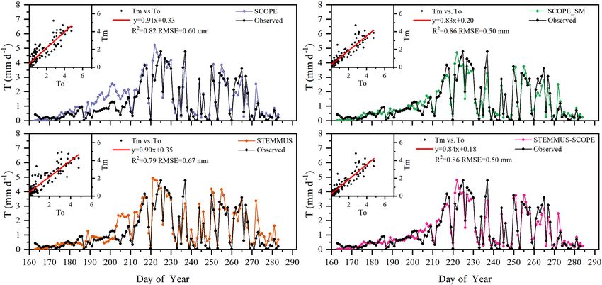
1382                              Y. Wang et al.: Integrated modeling of processes in the soil–plant–atmosphere continuum

Table 1. Continued.

                      Model     Sink term calculation of                            Root water uptake process
                                soil water balance
                                                            Hydraulic redistribu-    Compensatory uptake         Root distribution
                                                            tion (Richards and       (Jarvis, 2011)
                                                            Caldwell, 1987)
                      CABLE     Based on the gradient       Extreme case of CRWU     Following Darcy’s law       Empirical function
                                in water potentials be-                              for porous media flow
                                tween the leaf, stem,                                equations
                                and the weighted av-
                                erage of the soil (De
                                Kauwe et al., 2020)
       Crop models    APSIM     Potential transpiration     Not considered           Not considered              Empirical function
                                and water supply factor
                                but neglects root distri-
                                bution (Keating et al.,
                                2003)
                      CropSyst Difference in water po-      Not considered           Considered by the leaf      Linear decrease in soils
                               tential between the soil                              and soil water potential    with no limitations on
                               and the leaf, and a to-                                                           root exploration
                               tal soil–root–shoot con-
                               ductance (Stöckle et al.,
                               2003)
                      DSSAT     Water uptake per unit       Not considered           Water uptake per unit of    Using an        empirical
                                of root length is com-                               root length as a function   function
                                puted as an exponential                              of soil moisture
                                function, and the ac-
                                tual RWU is the mini-
                                mum of potential tran-
                                spiration and the max-
                                imum capacity of root
                                water uptake (Jones et
                                al., 2003)
                      EPIC      EPIC assumes that           Not considered           Not considered              Not considered
                                water is used prefer-
                                entially from the top
                                layers, and the potential
                                water supply rate de-
                                creases exponentially
                                downward (Williams et
                                al., 2014)
                      SWAP      Based on the potential      Not considered           Based on soil water po-     Function of      relative
                                transpiration, root frac-                            tential                     rooting depth
                                tion, and an empiric
                                stress factor relation-
                                ship (van Dam, 2000)
                      WOFOST The simplest one, it cal-      Not considered           Not considered              Empirical function
                             culates water uptake as
                             a function of the root-
                             ing depth and the water
                             available at that root-
                             ing depth without re-
                             gard for the soil water
                             distribution with depth
                             (Supit et al., 1994)

Geosci. Model Dev., 14, 1379–1407, 2021                                                    https://doi.org/10.5194/gmd-14-1379-2021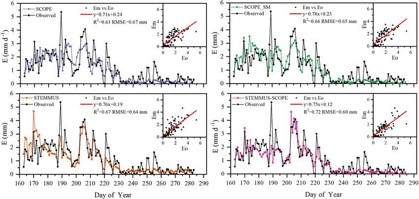
Y. Wang et al.: Integrated modeling of processes in the soil–plant–atmosphere continuum                                           1383

Table 1. Continued.

             Model      Sink term calculation of                            Root water uptake process
                        soil water balance
                                                    Hydraulic redistribu-    Compensatory uptake        Root distribution
                                                    tion (Richards and       (Jarvis, 2011)
                                                    Caldwell, 1987)
             SPACSYS According to empirical         Not considered           Not considered             1D (empirical function)
                     root length density dis-                                                           or 3D root system (pro-
                     tribution in a soil layer,                                                         cess based)
                     potential transpiration,
                     and soil moisture (Wu
                     et al., 2005)
             STICS      Based on the potential      Not considered           Not considered             1D root length density
                        transpiration, root frac-                                                       profile
                        tion, and soil water dis-
                        tribution, but not pro-
                        cess based (Beaudoin et
                        al., 2009)

2     Methodology and data                                            concept. Appendix A1 lists the main equations for calculat-
                                                                      ing the water stress factor within SCOPE (Bayat et al., 2019),
2.1    SCOPE and SCOPE_SM models                                      and the reader is referred to Van der Tol et al. (2009) for a de-
                                                                      tailed formulation of SCOPE.
SCOPE is a radiative transfer and energy balance model (Van              SCOPE_SM provides the basic framework to couple
der Tol et al., 2009). It simulates the transfer of optical, ther-    SCOPE with a soil process model. However, both SCOPE
mal, and fluorescent radiation in the vegetation canopy and           and SCOPE_SM ignored the soil heat and mass transfer pro-
computes ET using an energy balance routine. SCOPE in-                cesses and the dynamics of root growth. This can be over-
cludes a radiative transfer module for incident solar and sky         come by introducing the STEMMUS model.
radiation to calculate the top-of-canopy outgoing radiation
spectrum, net radiation, and absorbed photosynthetically ac-
tive radiation (aPAR); a radiative transfer module for ther-          2.2    STEMMUS model
mal radiation emitted by soil and vegetation to calculate the
top-of-canopy outgoing thermal radiation and net radiation;
an energy balance module for latent heat, sensible heat, and          The STEMMUS model is a two-phase mass and heat transfer
soil heat flux; and a radiative module for chlorophyll fluo-          model with explicit consideration of the coupled liquid, va-
rescence to calculate the top-of-canopy SIF (the observation          por, dry air, and heat transfer in unsaturated soil (Zeng et
zenith angle was set as 0◦ in this study).                            al., 2011a, b; Zeng and Su, 2013; Yu et al., 2016, 2018).
   Compared with other radiative transfer models that sim-            STEMMUS provides a comprehensive description of water
plify the radiative transfer processes based on Beer’s law,           and heat transfer in the unsaturated soil, which can compen-
SCOPE has well-developed radiative transfer modules that              sate for what is currently neglected in SCOPE. In STEM-
consider the various leaf orientation and multiple scattering.        MUS, the soil layers can be set in a flexible manner, which is
SCOPE can provide detailed information about the net radi-            an improvement on the previous SPAC model that only con-
ation of every leaf within the canopy. Furthermore, SCOPE             sidered the whole root zone soil water content as fixed layers
incorporates an energy balance model that predicts not only           (Williams et al., 1996). The water and heat transfer processes
the temperature of leaf but also the soil surface temper-             are vital for vegetation phenology development as well as
ature (i.e., a vital boundary condition needed by STEM-               freeze–thaw processes. The boundary condition needed by
MUS). In the original SCOPE model, soil is treated in a very          STEMMUS includes surface soil temperature, which is the
simple way with several empirical functions describing the            output of SCOPE. In addition, STEMMUS already contains
ground heat storage. Later, Bayat et al. (2019) extended the          an empirical equation to calculate root water uptake and a
SCOPE model by including the moisture effects on the vege-            simplified root growth module to calculate root fraction pro-
tation canopy, which resulted in the SCOPE_SM model. This             file. As such, STEMMUS has an ideal model structure to
model takes soil moisture as input and predicts the effects on        be coupled with SCOPE. The main governing equations of
several processes of the vegetation canopy using the SPAC             STEMMUS are listed in Appendix A2.

https://doi.org/10.5194/gmd-14-1379-2021                                                 Geosci. Model Dev., 14, 1379–1407, 2021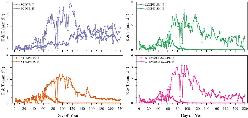
1384                             Y. Wang et al.: Integrated modeling of processes in the soil–plant–atmosphere continuum

2.3    Dynamic root growth and root water uptake                    et al. (2016). Although the behavior of plant stomata is in-
                                                                    fluenced by environmental factors, the potential water use
To obtain the root resistance of each soil layer, we incorpo-       efficiency (uWUEp , g C hPa0.5 (kg H2 O)−1 ) at the stomatal
rated a root growth module to simulate the root length density      scale in the ecosystem with a homogeneous underlying sur-
profile (see Appendix A3). The simulation of root growth            face is assumed to be nearly constant, and variations in ac-
refers to the root growth module in the INRA STICS crop             tual uWUE (g C hPa0.5 (kg H2 O)−1 ) can be attributed to the
growth model (Beaudoin et al., 2009), which includes the            soil evaporation (Zhou et al., 2016). Thus, the method can
calculations of root front growth and root length growth. The       be used to estimate T and E with the quantities of ET,
root front growth is a function of temperature, with the depth      uWUE, and uWUEp . Another assumption of this method is
of the root front beginning at the sowing depth for sown            that the ecosystem T is equal to ET at some growth stages, so
crops and at an initial value for transplanted crops or peren-      uWUEp√can be estimated using the upper bound of the ratio
nial crops (Beaudoin et al., 2009). The root length growth is       of GPP VPD to ET (here VPD refers to the vapor pressure
calculated in each soil layer, considering the net assimilation     deficit; Zhou et al., 2014, 2016).
rate and the allocation fraction of net assimilation to root,          Zhou et al.
                                                                                 √ (2016) used the 95th quantile regression be-
which is, in turn, a function of leaf area index (LAI) and root     tween GPP VPD and ET to estimate uWUEp , and they
zone water content (Krinner et al., 2005). The root length          showed that the 95th quantile regression for uWUEp at flux
density profile is then used to calculate the root resistance to    tower sites was consistent with the uWUE derived at the
water flow radially across the roots, soil hydraulic resistance,    leaf scale for different ecosystems. In addition, the variabil-
and plant axial resistance to flow from the soil to the leaves      ity in seasonal and interannual uWUEp was relatively small
(see Appendix A4).                                                  for a homogeneous canopy. Therefore, the calculations of
                                                                    uWUEp , uWUE, and T at the ecosystem scale were as fol-
2.4    STEMMUS–SCOPE v1.0.0 coupling                                lows:
                                                                                     √
The coupling starts with an initial soil moisture (SM) profile                  GPP VPD
                                                                    uWUEp =                                                    (1)
simulated by STEMMUS, which enables the calculation of
                                                                                    √T
the water stress factor as a reduction factor of the maximum                   GPP VPD
carboxylation rate (Vcmax ). SCOPE v1.73 is then used to cal-       uWUE =                                                     (2)
                                                                                    ET
culate net photosynthesis (An ) or gross primary productivity        T       uWUE
(GPP), soil respiration (Rs ), energy fluxes (net radiation, Rn ;        =          .                                          (3)
                                                                    ET uWUEp
latent heat, LE; sensible heat, H ; and soil heat flux, G), tran-
spiration (T ), and SIF, which is passed to STEMMUS as the          The calculation of the VPD was based on air temperature
root water uptake (RWU). Then, the gross primary produc-            and relative humidity data, and the method of gap-filling was
tion (GPP) can be calculated based on An . Surface soil mois-       the marginal distribution sampling (MDS) method proposed
ture is also used in calculating soil surface resistance and then   by Reichstein et al. (2005). To calculate GPP, the complete
calculating soil evaporation (E) . Furthermore, SCOPE can           series of net ecosystem exchange (NEE) was partitioned into
calculate soil surface temperature (Ts0 ) based on energy bal-      gross primary production (GPP) and respiration (Re) using
ance, which is subsequently used as the top boundary condi-         the method proposed by Reichstein et al. (2005). Finally, ET
tion of STEMMUS, and leaf water potential (LWP), which              was calculated using the latent heat flux and air temperature.
is a parameter to reflect plant water status, can be calculated     Based on GPP, ET, and VPD data, T can be calculated using
through iteration. Based on RWU, STEMMUS calculates the             the method proposed by Zhou et al. (2016).
soil moisture in each layer at the end of the time step, and
the new soil moisture profile will be the soil moisture at the      2.6   Study site and data description
beginning of next time step, which is repeated as such until
the end of simulation period. The time step of STEMMUS–             To evaluate the performance of STEMMUS–SCOPE in mod-
SCOPE is flexible, and the time step used in this study was         eling ecohydrological processes, simulation was conducted
30 min. Figure 1 shows the coupling scheme of STEMMUS               to compare STEMMUS–SCOPE with SCOPE, SCOPE_SM,
and SCOPE, and Table B1 in the Appendix shows all of the            and STEMMUS using observations over a C4 cropland (sum-
parameter values used in this study.                                mer maize: from 11 June to 10 October 2017) at the Yangling
                                                                    station (34◦ 170 N, 108◦ 040 E; 521 m a.s.l.) and a C3 grass-
2.5    Evapotranspiration partitioning                              land at the Vaira Ranch (US-Var) FLUXNET site (38◦ 250 N,
                                                                    120◦ 570 W; 129 m a.s.l.; annual grasses: from 1 June to 8 Au-
Most studies in partitioning evapotranspiration (ET) use sap        gust 2004). The seasonal variation in precipitation, irrigation,
flow and microlysimeter data from in situ measurements. In          and SM for these two sites are presented in Fig. 2, and the dif-
this study, we used a simple and practical method to sepa-          ferences in soil surface resistance, water stress factor (WSF),
rate evaporation (E) and transpiration (T ) proposed by Zhou        ET, photosynthesis, soil surface temperature (Ts0 ), root water

Geosci. Model Dev., 14, 1379–1407, 2021                                             https://doi.org/10.5194/gmd-14-1379-2021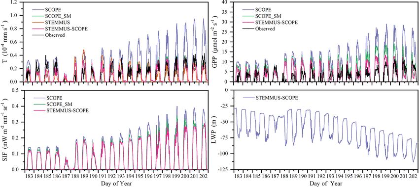
Y. Wang et al.: Integrated modeling of processes in the soil–plant–atmosphere continuum                                  1385

Figure 1. The coupling scheme of STEMMUS–SCOPE. Explanations for the symbols are given in Table B1 in the Appendix.

uptake (RWU), and leaf water potential (LWP) between these        2.7   Performance metrics
four models are presented in Table 2. In this study, the LAI
data of the Vaira Ranch (US-Var) FLUXNET site were from           The metrics used to evaluate the performance of the cou-
the MODIS 8 d LAI product instead of the field-measured           pled STEMMUS–SCOPE model include the (1) root-mean-
LAI used by Bayat et al. (2019). For the soil water content       square error (RMSE), (2) coefficient of determination (R 2 ),
employed by SCOPE_SM, the averaged root zone soil mois-           and (3) the index of agreement (d). They are calculated as
ture was used for Yangling station, and the soil moisture at      follows:
10 cm depth was used for the Vaira Ranch site. For more de-
tailed descriptions of these sites and data, the reader is re-
ferred to Wang et al. (2019, 2020a) and Bayat et al. (2018,
2019).

https://doi.org/10.5194/gmd-14-1379-2021                                            Geosci. Model Dev., 14, 1379–1407, 2021
1386                               Y. Wang et al.: Integrated modeling of processes in the soil–plant–atmosphere continuum

Figure 2. Seasonal variation in precipitation (P ); irrigation (I ); soil moisture at 2 (SM 2), 20 (SM 20), and 40 cm depth (SM 40); leaf area
index (LAI); and canopy height (hc ) for (a) maize cropland at Yangling station and (b) grassland at the Vaira Ranch (US-Var) FLUXNET
site.

Table 2. Main differences among SCOPE, SCOPE_SM, STEMMUS, and STEMMUS–SCOPE. The reader is referred to Table B1 in the
Appendix for a description of the abbreviations used in this table.

                               SCOPE                       SCOPE_SM                   STEMMUS                    STEMMUS–SCOPE
    Source                     Van der Tol et al. (2009)   Bayat et al. (2019)        Zeng and Su (2013)         This study
    Soil surface resistance    Set SM as constant or       Field-measured surface     Simulated surface SM       Simulated surface SM
    calculation                field-measured surface      SM                         by itself                  by itself
                               SM
    WSF calculation            Set SM as constant          Field-measured SM          Simulated SM by itself     Simulated SM by itself
    ET calculation             Process based (analogy      Process based (analogy     Penman–Monteith            Process based (analogy
                               with Ohm’s law)             with Ohm’s law)            model or FAO dual          with Ohm’s law)
                                                                                      crop coefficient method
    Photosynthesis             Farquhar and Collatz        Farquhar and Collatz       Absent                     Farquhar and Collatz
                               model                       model                                                 model
    Radiation transfer         SAIL4 model                 SAIL4 model                Based on Beer’s law        SAIL4 model
    Ts0                        Simulated by itself         Simulated by itself        Field measured             Simulated by itself
    RWU calculation            Absent                      Absent                     Based on potential T ,     Based on leaf and soil
                                                                                      root fraction, and soil    water potential
                                                                                      moisture profile
    LWP calculation            Absent                      Calculated by iteration    Absent                     Calculated by iteration
    Root growth                Absent                      Absent                     Empirical model            Process-based model

Geosci. Model Dev., 14, 1379–1407, 2021                                                    https://doi.org/10.5194/gmd-14-1379-2021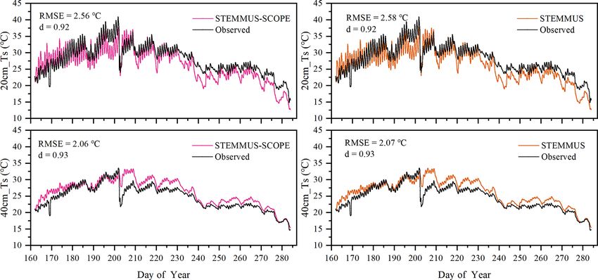
Y. Wang et al.: Integrated modeling of processes in the soil–plant–atmosphere continuum 1387
3.2 Soil temperature modeling
v
u n
u1 X Similar to soil moisture, only soil temperatures (Ts ) sim-
RMSE = t (Pi − Oi )2 , (4) ulated by STEMMUS and STEMMUS–SCOPE at 20 and
n i=1
40 cm depth at the Yangling site are shown in Fig. 4. In gen-
n
P
2 eral, both models can capture the dynamics of soil temper-
(Pi − P̄ )(Oi − Ō) ature well. For the simulation of temperature at 20 cm, the
i=1
2
R = n , (5) RMSE values were 2.56 and 2.58 ◦ C and the d values were
(Pi − P̄ )2 ni=1 (Oi − Ō)2 0.92 and 0.92 for STEMMUS and STEMMUS–SCOPE, re-
P P
i=1 spectively. For the simulation of temperature at 40 cm, the
n RMSE values were 2.06 and 2.07 ◦ C and the d values were
(Pi − Oi )2
P
i=1
0.93 and 0.93, respectively. These results indicate that both
d = 1− n , (6) models can simulate soil temperature well. However, some
( Pi − Ō + Oi − Ō )2
P
differences also exist between the simulation and observa-
i=1 tions. The largest difference occurred on DOY (day of year)
where Pi is the ith predicted value, Oi is the ith observed 202, when the field was irrigated using the flood irrigation
value, Ō is the average of the observed values, and n is the method. This irrigation activity may lead to boundary con-
number of samples. dition errors (i.e., for soil surface temperature), which can-
not be estimated well enough (e.g., there is no monitoring of
water temperature from the irrigation). Meanwhile, the mea-
3 Results and discussion surements may also have some errors during this period. The
fact that the observed soil temperature at 20 and 40 cm de-
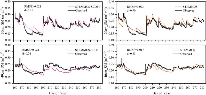
3.1 Soil moisture modeling creased to almost the same level at the same time indicates a
potential pathway for preferential flow in the field (see pre-
As the soil moisture profile was not available at the US- cipitation and irrigation on DOY 202 in Fig. 2), and the sen-
Var site, the comparisons of simulated soil moisture (SM) at sors captured this phenomenon. Nevertheless, the model cap-
Yangling station using STEMMUS and STEMMUS–SCOPE tures the soil temperature dynamics.
with observed values are presented in Fig. 3. For the simula-
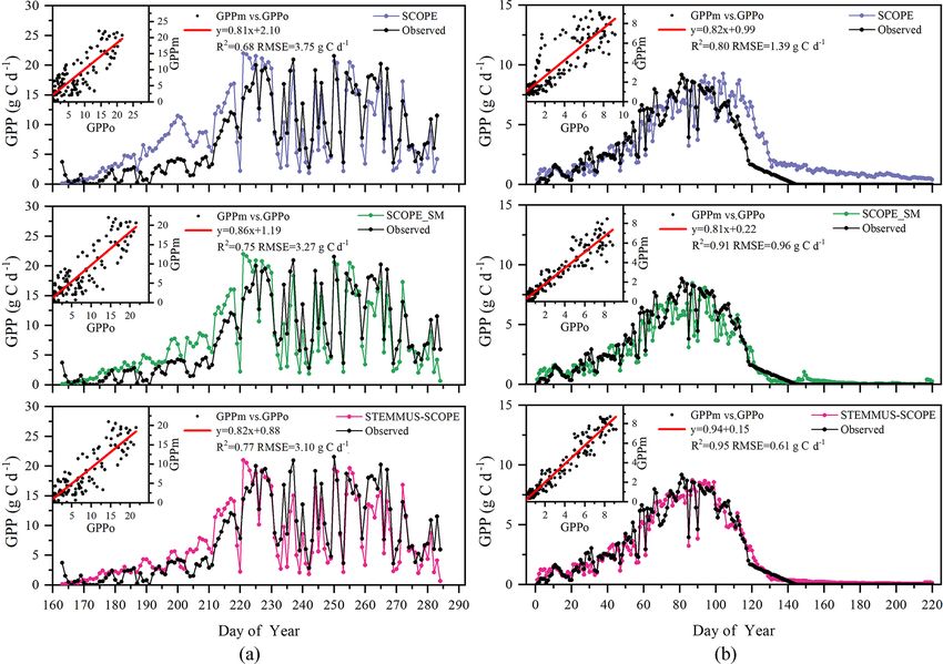
tion of soil moisture at 20 cm, the RMSE values were 0.023 3.3 Energy balance modeling
and 0.021 and the d values were 0.90 and 0.91 for STEM-
MUS and STEMMUS–SCOPE, respectively. For the simula- Comparisons of the modeled and observed 30 min net ra-
tion of soil moisture at 40 cm, the RMSE values were 0.017 diation (Rn ), sensible heat flux (H ), latent heat flux (LE),
and 0.021 and the d values were 0.83 and 0.74, respectively. and soil heat flux (G) using SCOPE, SCOPE_SM, and
The simulated soil moisture at 20 cm depth agreed with the STEMMUS–SCOPE are presented in Fig. 5 (STEMMUS
observed values in terms of the seasonal pattern. Although uses Rn as driving data; therefore, it is not included in
a slight overestimation occurred at initial and late stages, the the comparison). For net radiation and soil heat flux, the
dynamics in soil moisture resulting from precipitation or irri- simulations of all three models show good agreement with
gation were well captured. Per the nature of the two models, the observations, and the coefficients of determination (R 2 )
the coupling of SCOPE with STEMMUS is not expected to for SCOPE, SCOPE_SM, and STEMMUS–SCOPE were
improve the simulation of soil moisture. However, compared 0.99, 1.00, and 0.99, respectively. For soil heat flux, the R 2
with SCOPE_SM, which used soil moisture measurements values for SCOPE, SCOPE_SM, and STEMMUS–SCOPE
as inputs, the coupled STEMMUS–SCOPE model improves were 0.81, 0.79, and 0.80, respectively. For latent heat
the simulation of soil moisture dynamics as measured. The flux, STEMMUS–SCOPE shows better performance than
deviation between the model simulations and the measure- SCOPE and SCOPE_SM, and the R 2 values for SCOPE,
ments can be attributed to the following two potential rea- SCOPE_SM, and STEMMUS–SCOPE were 0.82, 0.84, and
sons. First, the field observations contain errors to a certain 0.85, respectively. Furthermore, STEMMUS–SCOPE and
extent, and the soil moisture sensors may be not well cali- SCOPE_SM show similar performance in the simulation of
brated. Second, in this simulation, we assumed that the soil sensible heat flux, both of which were better than the perfor-
texture was homogeneous in the vertical profile, whereas, in mance of SCOPE; the R 2 values for SCOPE, SCOPE_SM,
reality, the soil properties (e.g., soil bulk density and satu- and STEMMUS–SCOPE were 0.70, 0.75, and 0.74, respec-
rated hydraulic conductivity) may vary with depth and at dif- tively.
ferent growth stages due to field management practices. For
example, the soil bulk density at 40 cm was much higher than
that at 20 cm due to the mechanical tillage, especially in the
early stage.
https://doi.org/10.5194/gmd-14-1379-2021 Geosci. Model Dev., 14, 1379–1407, 2021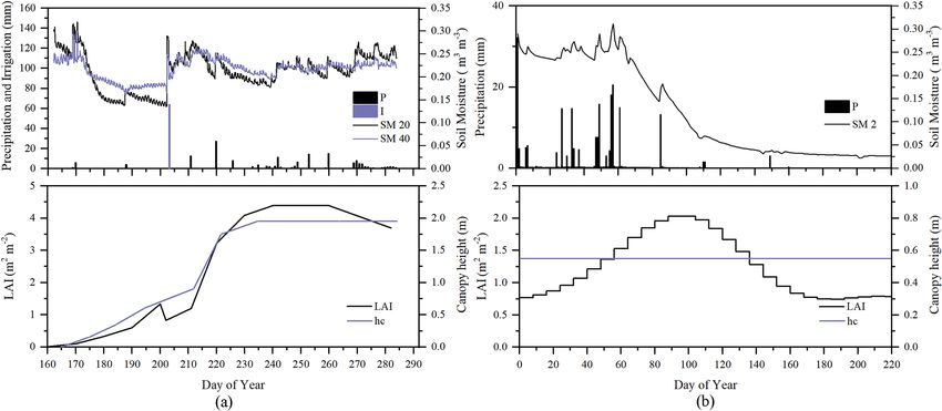
1388                            Y. Wang et al.: Integrated modeling of processes in the soil–plant–atmosphere continuum

Figure 3. Comparison of modeled and observed soil moisture at 20 (20 cm_SM) and 40 cm (40 cm_SM) depth for the maize cropland at
Yangling station.

Figure 4. Comparison of observed and modeled soil temperature at 20 (20 cm_Ts) and 40 cm (40 cm_Ts) depth for the maize cropland at
Yangling station.

3.4    Daily ET, T , and E modeling                                 and 0.89, and the RMSEs were 1.83, 0.63, 0.40, and
                                                                    0.34 mm d−1 , respectively. For the ET simulation by SCOPE,
Simulated daily evapotranspiration (ET) results by SCOPE,           there were large differences between simulations and ob-
SCOPE_SM, STEMMUS, and STEMMUS–SCOPE are pre-                       servations when the vegetation suffered water stress. For
sented in Fig. 6. For the Yangling station, the R 2 values          SCOPE_SM, STEMMUS, and STEMMUS–SCOPE, the
for SCOPE, SCOPE_SM, STEMMUS, and STEMMUS–                          simulated ET values were closer to observations when the
SCOPE were 0.76, 0.82, 0.80, and 0.81, and the RMSEs                vegetation experienced water stress because the dynamics
were 0.84, 0.69, 0.76, and 0.74 mm d−1 , respectively. For          of soil moisture was included in the model. This indicates
the US-Var station, the R 2 values for SCOPE, SCOPE_SM,             that STEMMUS–SCOPE, STEMMUS, and SCOPE_SM can
STEMMUS, and STEMMUS–SCOPE were 0.10, 0.66, 0.84,

Geosci. Model Dev., 14, 1379–1407, 2021                                             https://doi.org/10.5194/gmd-14-1379-2021
Y. Wang et al.: Integrated modeling of processes in the soil–plant–atmosphere continuum 1389 Figure 5. Comparison of modeled and observed 30 min net radiation (Rn ), latent heat (LE), sensible heat (H ), and soil heat flux (G) by SCOPE, SCOPE_SM, and STEMMUS–SCOPE at Yangling station. The subscripts “_m” and “_o” in each plot indicate modeled and observed quantities, respectively. The regression line is indicated in red, and the corresponding regression equation and R 2 value are given. predict ET with a relatively higher accuracy, especially when RMSEs were 0.60, 0.50, 0.67, and 0.50 mm d−1 , for SCOPE, the maize was under water stress (DOY 183–202 at Yan- SCOPE_SM, STEMMUS, and STEMMUS–SCOPE, respec- gling station and DOY 90–220 at the US-Var site), and tively. Because it ignored the effect of water stress on tran- STEMMUS–SCOPE and SCOPE_SM performed similarly spiration, SCOPE failed to simulate transpiration accurately well. It is noteworthy that although STEMMUS considered when the vegetation experienced water stress. As shown in the effect of soil moisture on ET, the accuracy of STEM- Fig. 6a, SCOPE overestimated transpiration for the maize MUS was lower than that of the coupled model (see Fig. 6). cropland at Yangling station from DOY 183 to 202 during the The possible reason for this is the better representation of water stress period. Compared with SCOPE, SCOPE_SM, transpiration in the SCOPE model (see Fig. 7), which sep- STEMMUS, and STEMMUS–SCOPE can capture the re- arates the canopy into 60 layers, whereas STEMMUS only duction in transpiration during the dry period. The perfor- treats the canopy as one layer. Moreover, the coupled model mance of STEMMUS–SCOPE and SCOPE_SM was also performed better for the grassland than for maize cropland. better than that of STEMMUS. The possible reason for this The reason for this is that the grassland simulation used the is the more processed-based consideration of the radiative dynamic Vcmax data, whereas the maize simulation used a transfer and energy balance at the leaf level in the cou- constant Vcmax data. pled STEMMUS–SCOPE model (as in SCOPE_SM) and The modeled and observed daily transpiration at the maize the more accurate root water uptake (compared with that cropland are presented in Fig. 7, and the modeled transpi- in SCOPE_SM). Nevertheless, STEMMUS–SCOPE slightly ration at the grassland site is presented in Fig. 8. For Yan- underestimated transpiration when the plant was undergo- gling station, the R 2 values between the simulated and ob- ing severe water stress and slightly overestimated it after the served transpiration were 0.82, 0.86, 0.79, and 0.86, and the field was irrigated. This is mainly because the actual Vcmax https://doi.org/10.5194/gmd-14-1379-2021 Geosci. Model Dev., 14, 1379–1407, 2021
1390                             Y. Wang et al.: Integrated modeling of processes in the soil–plant–atmosphere continuum

Figure 6. Comparison of modeled and observed daily evapotranspiration (ET) for (a) maize cropland at Yangling station and (b) grassland
at the Vaira Ranch (US-Var) FLUXNET site (ETm denotes modeled ET, and ETo denotes observed ET).

was not only influenced by drought but was also related to            from SCOPE and SCOPE_SM were both much higher than
the leaf nitrogen content (Xu and Baldocchi, 2003), which             those from STEMMUS and STEMMUS–SCOPE. The rea-
was not considered in the maize cropland simulation. Al-              son for the better performance of the coupled model for the
though measured T at the grassland was not available, we              grassland (Fig. 6b) is that it also considers the effect of the
compared modeled T from the four models (Fig. 7). During              leaf chlorophyll content (Cab ) on Vcmax , in addition to a more
the wet season (before DOY 85), the modeled T values from             detailed consideration of water stress as discussed above for
SCOPE, SCOPE_SM, and STEMMUS–SCOPE were simi-                         the maize cropland.
lar and were higher than that from STEMMUS from DOY 64                   As shown in Fig. 9 for soil evaporation at Yangling station,
to 82. During the dry season (after DOY 85), due to the sim-          the simulated values from STEMMUS–SCOPE are closer to
plified consideration of soil processes, the modeled T values         the observations than those from other models. When using

Geosci. Model Dev., 14, 1379–1407, 2021                                                https://doi.org/10.5194/gmd-14-1379-2021
Y. Wang et al.: Integrated modeling of processes in the soil–plant–atmosphere continuum                                             1391

Figure 7. Comparison of modeled and observed daily plant transpiration (T ) for the maize cropland at Yangling station (Tm denotes modeled
T , and To denotes observed T ).

Figure 8. Comparison of modeled daily transpiration (T ) and soil evaporation (E) for grassland at the Vaira Ranch (US-Var) FLUXNET site
(T denotes transpiration, and E denotes soil evaporation).

SCOPE to simulate soil evaporation, the soil moisture is set           and soil evaporation. Although STEMMUS can capture vari-
as constant (i.e., 0.25 m3 m−3 ). Therefore, SCOPE generally           ation in soil evaporation reasonably well, it has a higher
underestimates soil evaporation when soil moisture is higher           RMSE than STEMMUS–SCOPE. This is probably attributed
than 0.25 and overestimates it when it is lower than 0.25.             to the comprehensive consideration of radiation transfer in
Here, we use the average soil moisture at the root zone sim-           SCOPE, which is lacking in STEMMUS. Consequently, the
ulated by STEMMUS–SCOPE as the input data for SCOPE                    simulation of soil net radiation by the coupled model was
and SCOPE_SM in order to calculate soil surface resistance             more accurate than that from STEMMUS alone. The RMSE

https://doi.org/10.5194/gmd-14-1379-2021                                                   Geosci. Model Dev., 14, 1379–1407, 2021
1392 Y. Wang et al.: Integrated modeling of processes in the soil–plant–atmosphere continuum
Figure 9. Comparison of modeled and observed daily soil evaporation (E) at Yangling station (Em denotes modeled E, and Eo denotes
observed E).
value for STEMMUS–SCOPE was 0.60 mm d−1 , which was in STEMMUS–SCOPE and SCOPE_SM, the simulation of
lower than those from the other three models (0.67, 0.65, GPP was improved in both models. For Yangling station, the
and 0.64 mm d−1 , respectively). For STEMMUS–SCOPE, consistency between simulated and observed GPP at mid
the major differences between simulations and observations and late stages was higher than that at early and rapid growth
occurred on rainy or irrigation days (see Fig. 2a), which may stages. The difference usually occurred when soil mois-
be caused by errors in the estimated soil surface resistance ture increased. For the US-Var site, STEMMUS–SCOPE
during these periods or the uncertainty of the ET partition- simulated GPP well during the whole period, whereas
ing method. The uncertainty of the ET partitioning method SCOPE_SM slightly underestimated GPP around DOY 80
(Zhou et al., 2016) was mainly caused by (1) the uncertainty when this site transits from the wet season to the dry season.
in the partitioning of GPP (less than 10 %) and Re based This indicates that only using the surface SM cannot reflect
on NEE, which would result in some uncertainty in uWUE; the actual root zone SM when the vegetation is experiencing
(2) due to the seasonal variation in the atmospheric CO2 con- moderate water stress. Under such conditions, the hydraulic
centration – the assumption of uWUEp being constant would redistribution (HR) and compensatory root water uptake
cause some uncertainty (less than 3 %); (3) the assumption (CRWU) process enable the vegetation to utilize the water in
of T being equal to ET sometimes during the growing sea- the deep soil layer. Only using the surface soil water content
son would cause some uncertainty when vegetation is sparse. to calculate RWU in SCOPE_SM ignored the effect of the
Because the observed E at the US-Var site was not avail- HR and CRWU process, and the effect of water stress was
able, a comparison of only modeled E is shown in Fig. 8, in overestimated. However, the surface soil moisture can reflect
which SCOPE modeled unrealistic E during the dry season, root zone soil moisture well when the vegetation is not under
whereas the modeled E values from SCOPE_SM, STEM- water stress or severe water stress. A similar underestimation
MUS, and STEMMUS–SCOPE were consistent due to the of GPP was also found by Bayat et al. (2019).
use the simulated surface SM as the input for soil evapora-
tion calculation. 3.6 Simulation of leaf water potential (LWP), water
stress factor (WSF), and root length density (RLD)
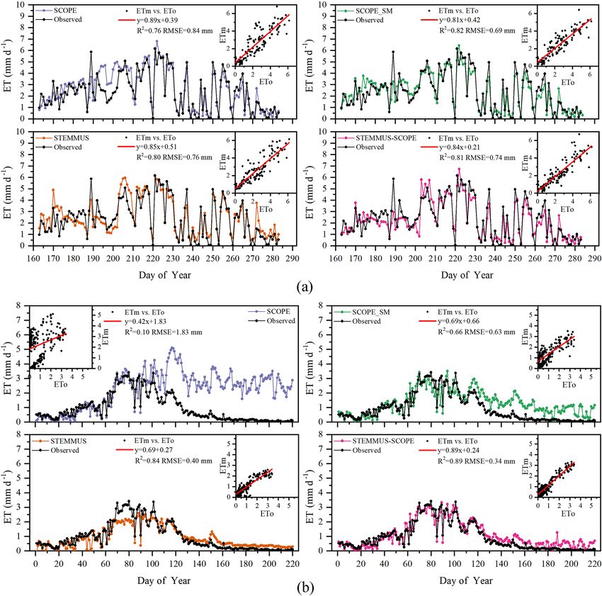
3.5 Daily GPP modeling
The simulated 30 min leaf water potential and water stress
Simulated GPP from SCOPE, SCOPE_SM, and factor at Yangling station are presented in Fig. 11. The leaf
STEMMUS–SCOPE and observed GPP are presented water potential was lower when vegetation was suffering wa-
in Fig. 10. As shown, similar to the simulation of tran- ter stress compared with other periods. The reason for this is
spiration, SCOPE cannot respond to water stress when that soil water potential is low due to the low soil moisture,
simulating GPP. After introducing a soil water stress factor and plants need to maintain an even lower leaf water poten-
Geosci. Model Dev., 14, 1379–1407, 2021 https://doi.org/10.5194/gmd-14-1379-2021Y. Wang et al.: Integrated modeling of processes in the soil–plant–atmosphere continuum 1393 Figure 10. Comparison of modeled and observed daily gross primary production (GPP) for (a) maize cropland at Yangling station and (b) grassland at the Vaira Ranch (US-Var) FLUXNET site (GPPm denotes modeled GPP, and GPPo denotes observed GPP). tial to suck water from the soil and transfer it to leaves. Dur- can be lower than −80 to −120 m when the vegetation was ing mid and late stages, the leaf water potential was sensitive under water stress and the leaves started curling, which was to transpiration demand due to the slowdown of root system similar to the simulated leaf water potential of maize in this growth. As continuous measurements of the leaf water po- study. Aston and Lawlor (1979) revealed the relationship be- tential are not available, we compared only the magnitude of tween transpiration, root water uptake, and leaf water po- simulated leaf water potential to measurements reported in tential of maize. These field studies found that leaf water the literature. potential was often very low and reached trough values at Many studies have measured midday leaf water poten- midday. Elfving et al. (1972) developed a water flux model tial or dawn leaf water potential. Fan et al. (2015) reported based on the SPAC system, evaluated it for orange trees, and that the leaf water potential of well-watered maize remained reported about −120 m for the trough value of leaf water po- high at between −73 and −88 m and that leaf water poten- tential under non-limiting environmental conditions, which tial would decrease when the soil water content was lower was slightly lower than the simulation in this study. than 80 % of field capacity. Martineau et al. (2017) reported In this study, the calculation of the water stress factor con- that the midday leaf water potential of well-watered maize sidered the effect of soil moisture and root distribution. The was around −0.82 MPa (about 84.8 m in water pressure severe water stress occurred from DOY 183 to 202, and the head; note that 0.1 MPa is equal to 10.339 m water pressure coupled model performed very well during this period. Due head) and that the midday leaf water potential decreased to to feedback, water stress can also influence root water uptake −1.3 MPa (about 134.4 m in water head) when the maize was and root growth and, consequently, influence soil moisture suffering water stress. Moreover, O’Toole and Cruz (1980) and root dynamics in next time step. This indicates that the studied the response of leaf water potential to water stress water stress equation used in this study can characterize the in rice and concluded that the leaf water potential of rice reduction in Vcmax reasonably well. https://doi.org/10.5194/gmd-14-1379-2021 Geosci. Model Dev., 14, 1379–1407, 2021
1394                               Y. Wang et al.: Integrated modeling of processes in the soil–plant–atmosphere continuum

Figure 11. Simulation of ψleaf (leaf water potential, m) and the WSF (water stress factor) at Yangling station. (The dotted lines represent the
range of midday leaf water potential reported at other sites.)

   Root length density is another vital parameter in calcu-               theless, the simulated root length density in our study was of
lating root water uptake. As shown in Table 3, the simu-                  an order of magnitude that was similar to the observations
lated peak root length density and maximum rooting depth                  from previous studies (Table 3).
of maize at Yangling station was comparable to the mea-
sured values from other sites. Many previous studies have                 3.7   Diurnal variation in T, GPP, SIF, and LWP
revealed that root length density is influenced by soil mois-
ture, bulk density, tillage, and soil mineral nitrogen (Am-               Figure 12 shows the modeled and observed 30 min canopy
ato and Ritchie, 2002; Chassot et al., 2001; Schroder et al.,             transpiration (T ), gross primary production (GPP), solar-
1996). In this study, as we assumed that the soil was ho-                 induced fluorescence (SIF), and leaf water potential (LWP)
mogenous. STEMMUS–SCOPE considered the effect of soil                     from DOY 183 to 202 at Yangling station. The simulations by
moisture but neglected the effect of bulk density and soil                STEMMUS–SCOPE and SCOPE_SM were consistent with
mineral nitrogen. Amato and Ritchie (2002) also found a                   observations, whereas the simulated values from SCOPE
similar result to this study with respect to the root length              were much higher than observations. The performance of
density in a maize field. Peng et al. (2012) studied tempo-               STEMMUS–SCOPE and SCOPE_SM was consistent with
ral and spatial dynamics in the root length density of field-             that of SCOPE in the early morning and late afternoon,
grown maize and found that 80 % root length density was                   when photosynthesis was mainly limited by incident radia-
distributed at 0–30 cm depth with peak values from 0.86                   tion rather than by water stress, intercellular CO2 concentra-
to 1.00 cm cm−3 . Ning et al. (2015) also reported a simi-                tion, and Vcmax . At midday, with increasing incident radia-
lar observation of root length density. Chassot et al. (2001)             tion, photosynthesis was mainly limited by water stress and
and Qin et al. (2006) reported that root length density can               Vcmax , during which time the simulations by STEMMUS–
reach 1.59 cm cm−3 in the Swiss Midlands. In Stuttgart, Ger-              SCOPE and SCOPE_SM were much better than that by
many, Wiesler and Horst (1994) observed the root growth                   SCOPE. The diurnal variation in the observed and modeled
and nitrate utilization of maize under field conditions. The              GPP was similar to that of T . Due to the lack of observed
observed root length density was 2.45–2.80 cm cm−3 at 0–                  SIF, only the simulated SIF values were presented. As shown
30 cm depth, which was much higher than in other studies,                 in Fig. 12, the SIF values simulated by STEMMUS- SCOPE
and decreased to 0.01 cm cm−3 at 120–150 cm depth, which                  and SCOPE_SM were reduced when the vegetation was ex-
was consistent with the observations of Oikeh et al. (1999)               periencing water stress, which indicated that both the sim-
at Samaru, Nigeria. Zhuang et al. (2001b) proposed a scaling              ulated SIF from STEMMUS–SCOPE and SCOPE_SM can
model to estimate the distribution of the root length density             respond to water stress. However, the accuracy of the simu-
of field-grown maize. In their study, the measured root length            lated SIF requires further validation with field observations.
density in Tokyo, Japan, decreased from 0.4 to 0.95 cm cm−3                  Figure 13 shows the relationship among 30 min GPP, SIF,
in the top soil layer to about 0.1 cm cm−3 in the bottom layer.           and LWP on DOY 199 at Yangling station. There was a
Zhuang et al. (2001a) observed that the root length density               strong linear relationship between SIF and GPP when the
of maize was mainly distributed at 0–60 cm depth, and the                 maize was well-watered (Fig. 13a). However, SIF kept in-
maximum values were about 0.9 cm cm−3 . These studies in-                 creasing, whereas GPP tended to saturate when the maize
dicated that the root length density values were quite variable           was suffering water stress. This result is consistent with the
when this parameter was observed at different sites; never-               previous study conducted for cotton and tobacco leaves (Van

Geosci. Model Dev., 14, 1379–1407, 2021                                                     https://doi.org/10.5194/gmd-14-1379-2021
Y. Wang et al.: Integrated modeling of processes in the soil–plant–atmosphere continuum                                              1395

Table 3. Comparison of the peak root length density (RLD; cm cm−3 ) at Yangling station with that at other sites.

      Location                        Maximum root-       Peak RLD      Soil type      Bulk density       References
                                      ing depth (cm)      (cm cm−3 )                   (g cm−3 )
      Potenza, Italy                               100          0.84    Clay loam            1.59–1.69    Amato and Ritchie (2002)
      Beijing, China                                60          0.78    Silty loam                        Peng et al. (2012)
      Alize, Stuttgart, Germany                    150          2.45    Clay                    1.5–1.7   Wiesler and Horst (1994)
      Brummi, Stuttgart, Germany                   150          2.80    Clay                    1.5–1.7   Wiesler and Horst (1994)
      Swiss Midlands                               100          1.59    Sandy silt           1.21–1.55    Qin et al. (2006)
      Samaru, Nigeria                               90          2.78    Loamy soil           1.39–1.67    Oikeh et al. (1999)
      Tokyo, Japan                                  58          0.95    Sandy loam           0.61–0.80    Zhuang et al. (2001a, b)
      Yangling, China                              121          0.74    Sandy loam                 1.41   This study

Figure 12. Comparison of modeled and observed 30 min transpiration (T ), gross primary production (GPP), top-of-canopy solar-induced
fluorescence (SIF), and leaf water potential (LWP) at Yangling station.

der Tol et al., 2014). Because SCOPE_SM used the aver-                  studies should focus on the measurement of SIF, GPP, and
aged root zone SM and ignored vertical root and soil wa-                LWP simultaneously for different vegetation types across
ter distribution, it overestimated GPP and SIF. When the                different environmental conditions (radiation, soil moisture,
maize was experiencing drought, the LWP was maintained at               and CO2 concentration) to reveal how the water stress affects
a low level. With GPP and T increasing, the plant decreased             these relationships.
LWP in order to extract enough water from the root zone.
The SPAC system enabled STEMMUS–SCOPE to simulate                       3.8    Limitations that need to be overcome
30 min LWP. To better detect the response of simulated SIF
to simulated LWP, we chose a cloudless day (DOY 199), and               The new coupled model notably improved simulations of car-
a liner relationship between the simulated SIF and LWP was              bon and water fluxes when vegetation was suffering water
obtained (Fig. 13b). Sun et al. (2016) reported that the SIF–           stress. However, this study mainly aimed to improve the re-
soil moisture–drought relationship depended on variations in            sponse of SCOPE to drought by introducing the vertical soil
both absorbed PAR and fluorescence yield in response to wa-             water and root profile. Some critical processes were followed
ter stress, whereas the LWP can reflect both the effect of              that existed in SCOPE_SM and STEMMUS. As with any
absorbed PAR and the soil moisture status. The strong cor-              model, some modules in STEMMUS–SCOPE, such as plant
relation between GPP, LWP, and SIF indicates the potential              hydraulics and root growth, could be improved upon in future
for using SIF as an effective signal for characterizing the re-         development.
sponse of photosynthesis to water stress. In the future, more              First, to date many LSMs (e.g., CLM 5, Noah-MP, JULES,
                                                                        and CABLE) have incorporated a state-of-the-art plant hy-

https://doi.org/10.5194/gmd-14-1379-2021                                                    Geosci. Model Dev., 14, 1379–1407, 2021
1396 Y. Wang et al.: Integrated modeling of processes in the soil–plant–atmosphere continuum Figure 13. The relationship among gross primary production (GPP), top-of-canopy solar-induced fluorescence (SIF), and leaf water potential (LWP) on DOY 199: (a) GPP vs. SIF; (b) SIF vs. LWP. draulics model to replace the conventional empirical plant early morning, the low stomatal aperture was induced by low hydraulic model which was only based on the distribution PAR rather than by SM. Consequently, STEMMUS–SCOPE of SM and the fraction of roots (e.g., CLM 4.5 and CoLM; needs to introduce advanced hydraulics after the model has De Kauwe et al., 2015). Although STEMMUS–SCOPE inte- been tested in a wide range of ecosystems, particularly for grated a 1D root growth model and a relatively novel RWU vegetation exposed to frequent drought cycles or prolonged model, its hydraulics model followed that in SCOPE_SM and periods of severe drought events. It is important, however, ignored the most exciting recent advances in our understand- to note that explicit representations of plant hydraulics re- ing of plant hydraulics: hydraulic failure due to the loss of quire additional model parameters and increase the param- hydraulic conductivity owing to embolism and refilling for eterization burden. This is the most challenging limitation recovery from xylem embolism (McDowell et al., 2019). Be- to STEMMUS–SCOPE with respect to incorporating these cause STEMMUS–SCOPE performed well in maize crop- hydraulics models, and we have chosen a trade-off between land and grassland, the influence of embolism and refill- mechanism and practicality. ing on water transfer from the soil through vegetation to Second, as mentioned above, STEMMUS–SCOPE the atmosphere cannot be fully detected. The value of us- adapted the macroscopic RWU model and a simplified 1D ing plant water potential instead of soil water potential to root growth model in order to save on computational costs, constrain model predictions has been demonstrated in many although it predicted maximum root depth well, which is case studies (De Kauwe et al., 2020; Niu et al., 2020; Med- the most critical factor when calculating WSF and RWU. lyn et al., 2016; Xu et al., 2016; Williams et al., 1996). Niu Such a simplification would likely ease the migration of et al. (2020) followed the plant hydraulic model developed our model into larger-scale models, such as Earth system by Xu et al. (2016) and represented the plant stomatal wa- models. However, STEMMUS–SCOPE oversimplified ter stress factor as a function of the plant water storage. metabolic processes of the roots, including root exudates, CLM 5.0 also introduced a new formulation for WSF, which root maintenance respiration, root growth respiration, and is based on leaf water potential (ψleaf ) instead of soil wa- root turnover, which are also critical and have been incor- ter potential (ψsoil ; Kennedy et al., 2019). These new for- porated in Noah-MP (Niu et al., 2020). This simplification mulations based on plant water potential could offer sig- could result in uncertainties in modeling the root growth and nificant improvements for plant drought responses. Further- root water uptake. Meanwhile, there was no validation of more, STEMMUS–SCOPE presently does not account for the seasonal vertical root length distribution based on in situ plant water storage; this may result in underestimating morn- observations, which need to be validated in the next step. ing LE and overestimating afternoon LE. Some field observa- Furthermore, the model presently does not account for the tions have shown that the plant do not immediately respond feedback between hydraulic controls over carbon allocation when soil moisture is enhanced (Mackay et al., 2019), instead and the role of root growth on soil–plant hydraulics, which there are long lags, which were ignored in this study, between could also be considered in future model development. soil water recovery from drought and plant responses to the recovery. The WSF in STEMMUS–SCOPE directly comes from soil moisture and cannot reflect true stomatal response when vegetation is experiencing drought. For example, in Geosci. Model Dev., 14, 1379–1407, 2021 https://doi.org/10.5194/gmd-14-1379-2021
You can also read