Geometric Properties of Backdoored Neural Networks
←
→
Page content transcription
If your browser does not render page correctly, please read the page content below
Geometric Properties of Backdoored Neural Networks

                Dominic Carrano

                Electrical Engineering and Computer Sciences
                University of California, Berkeley

                Technical Report No. UCB/EECS-2021-78
                http://www2.eecs.berkeley.edu/Pubs/TechRpts/2021/EECS-2021-78.html

                May 14, 2021
Copyright © 2021, by the author(s).
All rights reserved.
Permission to make digital or hard copies of all or part of this work for
personal or classroom use is granted without fee provided that copies are
not made or distributed for profit or commercial advantage and that copies
bear this notice and the full citation on the first page. To copy otherwise, to
republish, to post on servers or to redistribute to lists, requires prior specific
permission.Geometric Properties of Backdoored Neural Networks
by Dominic Carrano
Research Project
Submitted to the Department of Electrical Engineering and Computer Sciences,
University of California at Berkeley, in partial satisfaction of the requirements for the
degree of Master of Science, Plan II.
Approval for the Report and Comprehensive Examination:
Committee:
Professor Kannan Ramchandran
Research Advisor
(Date)
*******
Professor Michael W. Mahoney
Second Reader
(Date)1
Abstract
Geometric Properties of Backdoored Neural Networks
by
Dominic Carrano
Master of Science in Electrical Engineering and Computer Sciences
University of California, Berkeley
Backdoor attacks recently brought a new class of deep neural network vulnerabilities to
light. In a backdoor attack, an adversary poisons a fraction of the model’s training data
with a backdoor trigger, flips those samples’ labels to some target class, and trains the model
on this poisoned dataset. By using the same backdoor trigger after an unsuspecting user
deploys the model, the adversary gains control over the deep neural network’s behavior. As
both theory and practice increasingly turn to transfer learning, where users download and
integrate massive pre-trained models into their setups, backdoor attacks present a serious
security threat. There are recently published attacks that can survive downstream fine-
tuning and even generate context-aware trigger patterns to evade outlier detection defenses.
Inspired by the observation that a backdoor trigger acts as a shortcut that samples can
take to cross a deep neural network’s decision boundary, we build off the rich literature
connecting a model’s adversarial robustness to its internal structure and show that the same
properties can be used to identify whether or not it contains a backdoor trigger. Specifically,
we demonstrate that backdooring a deep neural network thins and tilts its decision boundary,
resulting in a more sensitive and less robust classifier.
In addition to a simpler proof of concept demonstration for computer vision models on
the MNIST dataset, we build an end-to-end pipeline for distinguishing between clean and
backdoored models based on their boundary thickness and boundary tilting and evaluate
it on the TrojAI competition benchmark for NLP models. We hope that this thesis will
advance our understanding of the links between adversarial robustness and defending against
backdoor attacks, and also serve to inspire future research exploring the relationship between
adversarial perturbations and backdoor triggers.i I dedicate this thesis to my mother Carmen, for serving as my role model of what an engineer is, and for your sacrifices and selflessness; my father Christopher, my other role model of an engineer, for the six-star home-cooked meals, the endless laughs, and — of course — for making me ”check the box”; my grandparents Pamela, Donald, Elizabeth, and Anthony, for all your love and support; and my sister Isabella and brother Nicholas, for putting up with me and always keeping me on my toes.
ii

                                 Acknowledgments
    Even as a Bay Area native, I didn’t know just how much energy Berkeley had until I
started school here. You’d be hard pressed to find another place on Earth where you can
attend a talk on the future of computing given by a Turing Award laureate, buy a tie-dye
shirt from a street vendor, and enjoy a pizza with baked egg on it — all in the span of two
hours. But even better than Berkeley’s breadth of culture and food is the people that make
it the legendary place it is, and I want to acknowledge them here.
    It’s only appropriate that I begin with everyone directly involved in my research en-
deavors, and there’s no better place to start than with my advisor, Professor Kannan
Ramchandran. I first met Kannan in the fall of my junior year as a student in his EECS
126. From the first lecture he gave on Shannon’s theory of communication systems, I was
amazed by the clarity and intuition he brought to explaining technical concepts. As both
a teacher and an advisor, Kannan’s insistence on keeping things simple, thinking from first
principles, and using myriad visual examples to introduce new ideas have profoundly in-
fluenced both my presentation style and how I go about solving problems. His breadth of
technical knowledge amazes me, and I leave every one of our meetings refreshed with new
ideas of how to tackle whatever problems I was previously stuck on. Kannan has made me a
better student, teacher, researcher, and engineer, and I’m lucky to have him as an advisor.
    Turning now to the other member of my thesis committee, I’d like to thank Professor
Michael Mahoney. Earlier this year when I developed an interest in exploring AI security,
Michael welcomed me into his group — who had already been working in the area for several
months — with open arms. I’m constantly amazed at how many insightful questions he asks
at our weekly group meetings, drawing connections I don’t know that I ever would have.
I also thank Michael for graciously allowing me access to his group’s shared GPU cluster,
without which this project would have been computationally infeasible.
    Next, I’d like to thank my two closest collaborators on this project, Yaoqing Yang and
Swanand Kadhe. In addition to being seasoned researchers — and experts in adversarial
robustness and security, respectively, that I’m lucky to have as mentors — Yaoqing and
Swanand always make time to meet whenever I come across a new set of results or anything
else to discuss, and I always leave our meetings fresh with ideas. I especially thank Yaoqing
for pitching the idea of this project to me back in January, bringing Swanand and I into the
TrojAI competition group, and helping me get all set up with the compute resources and his
codebase. I’d also like to thank Francisco Utrera and Geoffrey Negiar for helping guide
several useful discussions throughout the course of working on this project.
    Rounding out the group of excellent researchers I’ve been fortunate enough to work
with during my time here is Vipul Gupta. When I first joined Kannan’s lab back in late
2018, Vipul took me in as his mentee, and we worked together on a project in distributed
computing that introduced me to what research was all about. I’m incredibly grateful for
everything he’s taught me and all the great conversations we’ve had over the past few years.
iii
Second, I want to acknowledge some of the main people who made my five semesters
as a TA such a uniquely amazing part of my education. Berkeley — especially the EECS
department — is known for the extreme levels of autonomy it gives its students, perhaps best
exemplified by how it lets undergrads help teach and run its courses. As my friend Suraj once
put it, the opportunity to work as a TA probably isn’t something the university would ever
advertise to high school students as a selling point, but it’s taught me just as much as my
research and coursework have. And for that, I have Professor Babak Ayazifar to thank.
In addition to teaching four of the courses I took as a student here, making him responsible
for a full 14 units’ worth of my education, Babak was crazy enough to hire me as his TA
three times and has served as an amazing mentor throughout my time here. He’s taught me
how to use breaks and an interactive presentation style to maintain audience attention, the
importance of being patient and accommodating, the value of clear and concise writing —
and don’t let me forget the em dash. Along with Kannan, I’m proud to call Babak one of
my two biggest role models of what a great teacher is.
While on the subject of being a TA, I have to thank two of my fellow EE 120 course
staff members, Jonathan Lee and Ilya Chugunov. Without diving into the catalog of
hilarious stories we’ve built up over the years, I’ll say that these two guys’ amazing work
ethic, dedication to our students, and sense of humor and sarcasm made the job as fun and
fulfilling as I could have ever asked for.
I’m extremely lucky to have been the recipient of a number of generous scholarships and
work opportunities throughout my time as an undergraduate and graduate student here
that helped me pay for school. I’ve especially benefited from the aforementioned teaching
assistantships in the EECS Department, for which I thank Professor Babak Ayazifar,
Professor Murat Arcak, and Professor Venkat Anantharam. I’d also like to men-
tion that this effort was supported by the Intelligence Advanced Research Projects Agency
(IARPA) under the contract W911NF20C0035. Our conclusions do not necessarily reflect
the position or the policy of our sponsors, and no official endorsement should be inferred.
From the EECS administration, I would like to thank Michael Sun for his help through-
out the past year in handling the MS program logistics, Bryan Jones for our meetings
throughout my undergrad years checking in to make sure I was on track to graduate, and
Eric Arvai for the countless hours of patient, generous assistance in managing all the lecture
recordings and YouTube playlists I was responsible for as a TA.
To my siblings, parents, and grandparents, please see the dedication. To all my other
relatives, friends, colleagues, and teachers: the confines of a Master’s thesis acknowledgments
section is far too limiting a forum to adequately express my gratitude to you all. Please know
that I do appreciate everything you’ve done for me.iv Contents Contents iv List of Figures vi List of Tables vii 1 Introduction 1 1.1 Main Contributions . . . . . . . . . . . . . . . . . . . . . . . . . . . . . . . . 2 2 Background and Related Work 3 2.1 Natural Language Processing . . . . . . . . . . . . . . . . . . . . . . . . . . 3 2.2 Adversarial Robustness . . . . . . . . . . . . . . . . . . . . . . . . . . . . . . 5 2.3 Backdoor Attacks . . . . . . . . . . . . . . . . . . . . . . . . . . . . . . . . . 6 3 Backdoored Vision Models: MNIST Proof of Concept 9 3.1 Experimental Setup . . . . . . . . . . . . . . . . . . . . . . . . . . . . . . . . 9 3.2 Method . . . . . . . . . . . . . . . . . . . . . . . . . . . . . . . . . . . . . . 11 3.3 Results . . . . . . . . . . . . . . . . . . . . . . . . . . . . . . . . . . . . . . . 11 4 Backdoored NLP Models: The TrojAI Competition 15 4.1 Experimental Setup . . . . . . . . . . . . . . . . . . . . . . . . . . . . . . . . 15 4.2 Exploring CLS Embeddings . . . . . . . . . . . . . . . . . . . . . . . . . . . 16 4.3 Method . . . . . . . . . . . . . . . . . . . . . . . . . . . . . . . . . . . . . . 17 4.4 Results . . . . . . . . . . . . . . . . . . . . . . . . . . . . . . . . . . . . . . . 20 5 Conclusion 21 5.1 Potential Directions for Future Research . . . . . . . . . . . . . . . . . . . . 21 A Notation 24 B Backdoor Attack (Formal) 25 C Boundary Thickness (Formal) 27
v

D Boundary Tilting (Formal)   30

Bibliography                  32
vi
List of Figures
2.1 Typical architecture of a sentiment classifer. In lightweight applications, including
all our NLP experiments, a common value of d is 768. . . . . . . . . . . . . . . . 4
2.2 Model robustness viewed through the lens of boundary tilting. . . . . . . . . . . 6
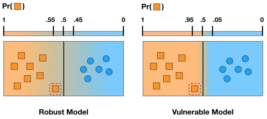
2.3 Model robustness measured with boundary thickness. Both models draw identical
decision boundaries — making them equally robust in the eyes of boundary tilting
— but the model on the right is 95% certain that the highlighted point is an orange
square despite how close it is to the decision boundary, whereas the model on the
left is only 55% certain. The model on the left has a thicker boundary, although
a higher cross-entropy loss. . . . . . . . . . . . . . . . . . . . . . . . . . . . . . . 7
2.4 Example of a backdoor attack on the MNIST dataset. The trigger pattern is a
square at the top left of an image of a 0, used to make the model predict that it’s
a 1. . . . . . . . . . . . . . . . . . . . . . . . . . . . . . . . . . . . . . . . . . . . 8
3.1 Examples of clean versus triggered samples for each of the three types of triggers
we consider. Note that for a one2one trigger, the 1’s class isn’t triggered, so the
image in the top right looks identical to the one to its left. . . . . . . . . . . . . 10
3.2 Results with a logistic regression clean reference model for boundary tilting; all
potentially poisoned models are CNNs. Each point represents a different random
seed. Note that the ”None” models are also CNNs, so this truly is a fair compari-
son where both the poisoned and clean models under inspection all have the same
architecture; only the reference model for computing boundary tilting directions
is logistic regression. . . . . . . . . . . . . . . . . . . . . . . . . . . . . . . . . . 12
3.3 Results with a CNN clean reference model for boundary tilting; all potentially
poisoned models are CNNs of the same architecture as the clean reference model.
Note that the thickness distributions are nearly identical to the previous figure’s,
since the only change here is the reference model used to generate adversarial
directions for comparison via boundary tilting. Each point represents a different
random seed. . . . . . . . . . . . . . . . . . . . . . . . . . . . . . . . . . . . . . 13
3.4 Universal adversarial perturbations of MNIST 0’s and 1’s for various clean and
backdoored models. Even without an explicit sparsity prior to guide the opti-
mization, the universal adversarial perturbation on the backdoored models closely
resembles the corresponding trigger pattern from Figure 3.1. All backdoored
models are CNNs. . . . . . . . . . . . . . . . . . . . . . . . . . . . . . . . . . . . 14vii
4.1 Unnormalized histogram of the `2 norm of each language model’s CLS embeddings
formed from 10K randomly sampled reviews, half positive and half negative.
As we go from left to right, both the mean and variance of the corresponding
distribution increases. . . . . . . . . . . . . . . . . . . . . . . . . . . . . . . . . 16
4.2 Stem plot of CLS(triggered) - CLS(clean). Each stem corresponds to an element
of the 768-dimensional vector. Column n corresponds to the pair of reviews in
row n of Table 4.1. The GPT-2 vectors aren’t sparse, their outliers just dominate
the plot. . . . . . . . . . . . . . . . . . . . . . . . . . . . . . . . . . . . . . . . . 17
List of Tables
4.1 Clean and triggered review pairs from the TrojAI Round 5 dataset. The trigger
word, phrase, or character is highlighted in yellow. Row n of this table corre-
sponds to the plots in column n of Figure 4.2. Note the semantic neutrality of
these triggers: none have a strong positive or negative sentiment associated with
them. . . . . . . . . . . . . . . . . . . . . . . . . . . . . . . . . . . . . . . . . . 18
4.2 Performance on TrojAI Round 5. A lower CE and higher AUC indicates a better
model. We averaged our final results over five random seeds to prevent any
one lucky or unlucky seed from skewing them. The state-of-the-art performance
reported here is from https://pages.nist.gov/trojai/docs/results.html. . 201
Chapter 1
Introduction
Since the seminal work of Alex Krizhevsky and others nearly a decade ago [1], deep neural
networks (DNNs) have exploded in popularity and been applied to problems spanning the
gamut from malware detection [2, 3] to machine translation [4, 5, 6, 7, 8]. However, as sci-
entists and engineers begin to integrate them into sensitive applications such as autonomous
driving [9, 10] and medical diagnosis [11], artificial intelligence (AI) researchers continue to
emphasize that DNNs are fundamentally pattern recognition systems: they find trends in
their training data that may be brittle and completely unintelligible to a human [12, 13],
and they’re often easily fooled by applying a small, barely perceptible perturbation to their
inputs [14, 15]. Perhaps even more concerning, several research groups have independently
shown that DNNs are vulnerable to backdoor attacks, where an adversary implants a hidden
trigger pattern in the model that they can exploit to control the model’s predictions [16, 17,
18]. Remarkably, these attacks can (1) succeed without affecting the model’s performance
on clean data, making them impossible to detect by measuring accuracy on a test set the
attacker is unaware of; (2) survive fine-tuning, where the user further trains the potentially
backdoored model to improve its performance after the attack, even if the attacker doesn’t
know what dataset the fine-tuning will be performed on [19]; and (3) embed the trigger
pattern in a context-aware, input-dependent way that evades test time anomaly detection
methods [20]. This is especially concerning given the recent rise in transfer learning for
natural language processing (NLP) applications, where an engineer downloads a pre-trained
model and uses it in their end-to-end system without any control over how it was trained.
Similar to adversarial attacks, backdoor attacks are an intriguing subfield of AI security
both due to the direct threat they pose — the potential untrustworthiness of a pre-trained
model, in the case of backdoors — and the opportunity they provide to better understand
DNN generalization behavior. As of May 2021, defending against backdoor attacks remains
an important open problem; no bulletproof defense currently exists. Several works have
proposed defenses based on test time anomaly detection [21, 22], but this is becoming an
increasingly impractical option — especially in NLP — as attackers have developed context-
aware trigger mechanisms that can, for example, embed a trigger word inside a sentence the
attacker generates as a continuation of the input text [20]. Another line of backdoor defensesCHAPTER 1. INTRODUCTION 2
essentially performs a ”malware scan” on the DNN and renders a verdict as to whether or
not it’s backdoored. However, these methods often heavily rely on a sparsity prior or explicit
hypothesis class for the trigger in order to achieve good performance [23, 24, 25], involve
a computationally intractable brute-force search through potential trigger phrases [19], or
risk lowering the model’s accuracy on clean data by removing neurons [26]. Developing a
principled approach based on few to no assumptions about the trigger function that focuses
on the backdoored model’s internal structure is a key step toward understanding backdoor
attacks across different DNN architectures and problem domains.
1.1 Main Contributions
In an effort toward understanding backdoored DNNs more fundamentally, we leverage the
rich literature on adversarial robustness to identify the differences between clean and back-
doored models’ decision boundaries. Specifically, we show that backdooring a model:
(1) thins its decision boundary, creating shortcuts that points can take to cross over to the
other side, and generally making the model’s predictions more sensitive; and
(2) tilts its decision boundary, altering the directions of its adversarial perturbations.
We do not assume knowledge of the trigger or access to the original training data, and
require only a modest number of clean inputs representative of the DNN’s problem domain
in addition to the pre-trained, potentially poisoned model under consideration. While the
geometry of a model’s decision boundary may not be the best or only feature for determining
if the model is backdoored, our main goal here is to study how these properties change as a
result of a backdoor attack. We’ve open-sourced the code from our TrojAI experiments so
that our work can be reproduced and extended.1 To the best of our knowledge, this is the
first work to analyze the boundary thickness or boundary tilting of a backdoored DNN.
1
https://github.com/dominiccarrano/backdoor-nn-geometry3
Chapter 2
Background and Related Work
2.1 Natural Language Processing
Most prototypical examples of classification systems involve computer vision tasks, where,
for instance, a model takes an image and outputs a semantic category describing the im-
age’s content, such as cat or dog. And there’s a good reason why: images, being arrays of
continuously-valued pixels, are readily used as the input to a deep neural network (DNN),
which learns patterns from data by solving a continuous optimization problem [27]. But
DNNs have also been successfully employed in a wide variety of natural language processing
(NLP) tasks — where the goal is to analyze text rather than images — with applications
ranging from part-of-speech tagging [28, 29, 30] to machine translation [4, 5, 6, 7, 8]. In
contrast to computer vision tasks, the input in an NLP problem comes from a large but
ultimately discrete space. This creates a barrier to entry for anyone interested in using a
DNN for an NLP task: deciding how to represent words as real-valued vectors, known as
embeddings, that the DNN can use as a part of its optimization.
The simplest option is to represent words using their indices within a vocabulary, known
as a one-hot encoding, but this fails to express any notion of word similarity: synonyms like
”great” and ”excellent” should be close together in this embedding space. Some of the first
widely adopted algorithms for generating word embeddings such as word2vec [31], GloVe
[32], and approaches based on neural language models [33] improved on one-hot encoding by
making use of context — the idea that a word’s embedding should depend on what other
words typically appear before or after it — but these methods were still limited by their
static nature and inability to handle homonyms. For example, the word2vec embedding of
the word ”ran” would be the same in the sentences ”I ran a marathon” and ”My code ran for
six hours yesterday” despite its vastly different meanings. The issue is that these approaches
learn a single embedding based on all the different contexts that they’ve ever seen ”ran”
appear in, and don’t allow the flexibility of a different embedding for ”ran” depending on
the sentence it shows up in. This is what makes them static. In contrast, today’s state-
of-the-art language models such as Google’s BERT [34] and its variants [35, 36], as well asCHAPTER 2. BACKGROUND AND RELATED WORK 4 Figure 2.1: Typical architecture of a sentiment classifer. In lightweight applications, includ- ing all our NLP experiments, a common value of d is 768. OpenAI’s GPT-n series models [37, 38, 39] overcome this limitation by producing context- aware word embeddings — ones that depend on the rest of the input sentence surrounding the word. These models typically have hundreds of millions (or even hundreds of billions [39]) of parameters, are trained on an unlabelled corpus of textual data containing billions of words, and produce plug-and-play embeddings ready for integration into NLP pipelines. As an example application of these massive-scale pre-trained language models, we’ll discuss sentiment classification next. Sentiment Classification In sentiment classification, we’re given a textual review (e.g., for a movie or product), and want to predict whether the review is positive or negative. The standard architecture of a sentiment classifier, shown in Figure 2.1, consists of one of the aforementioned language models which generates a sentence-level embedding — a single embedding vector describing the semantic content of the entire sentence, not just a single word — followed by a simple classifier (e.g., logistic regression) that’s trained on pairs of sentence-level embeddings and labels indicating if the review is positive or negative. This sentence-level embedding is known as a ”CLS” (CLaSsification) embedding when BERT or one of its variants is the language model of choice. GPT models don’t technically have a ”CLS” embedding in the same way BERT does; instead, we use the embedding from the last token of a GPT input as its sentence-level embedding, since GPT models are autoregressive and gradually build in context from the start of an input to its end. However, for convenience, we’ll refer to this sentence-level embedding as the review’s CLS embedding regardless of the language model.
CHAPTER 2. BACKGROUND AND RELATED WORK                                                       5

2.2     Adversarial Robustness
Around 2013, AI researchers discovered the now well-known phenomenon of adversarial
examples: inputs that have been perturbed in a carefully crafted way that is barely (if
at all) perceptible to humans, but cause a classifier to make an incorrect prediction [14].
Subsequent work demonstrated that (1) the same adversarial example can fool multiple
different classifiers, even if they have completely different architectures [15]; (2) a single
universal adversarial perturbation (UAP) exists that can, with high probability, fool a model
on any sample [40, 41]; and (3) adversarial examples exist in essentially all learned models,
even humans [42]. There are several algorithms available for computing adversarial examples
for a model given access to first-order information, ranging from the Fast Gradient Sign
Method (FGSM) [15], which is essentially a single step of gradient ascent, to stronger multi-
iteration attacks based on Projected Gradient Descent (PGD) [43]. However, it’s possible to
generate adversarial examples for a model with just black-box access by training a similar
surrogate model and transferring over the surrogate model’s adversarial examples [44, 45].
    One of the best known defenses against adversarial examples is adversarial training,
introduced in [15]: generate adversarial examples (e.g., using FGSM or PGD) for a model,
and train it to recognize them as being from the same class as the unperturbed image. This
can be viewed as solving a robust optimization problem, minimizing the model’s loss over an
inner maximization that generates the adversarial examples to attempt to fool the model.
However, as noted by [46, 47], this only provides a defense against the threat model used to
perform the adversarial training. Additionally, the robustness offered by adversarial training
typically comes at the price of lower classification accuracy on clean examples. Despite being
a hot topic of AI research, defending against adversarial examples remains an important open
problem, although one that’s out of scope for us here. Two independent lines of work that
we’ll now review — boundary tilting and boundary thickness — have, rather than attempt
to defend against adversarial examples, aimed to characterize how robust a learning model
is against them based on the geometry of its decision boundary.

Boundary Tilting
The idea behind boundary tilting [48] is that a decision boundary to separate two classes
should be drawn such that to cross the boundary, a point must move in a direction that
changes its semantic meaning. For example, the model in the left of Figure 2.2 has this
property: to make the model predict an orange square as a blue circle, the orange square
has to move closer to the cluster of blue circles. In contrast, the model on the right of
Figure 2.2 has a heavily tilted decision boundary, creating the existence of points like the
one highlighted in red that, despite being closer to the cluster of blue circles, is classified
as an orange square. Far from being limited to linear models, boundary tilting can easily
be measured for classifiers with nonlinear decision boundaries by considering the model’s
adversarial perturbations. For a more formal explanation, see Appendix D.
CHAPTER 2. BACKGROUND AND RELATED WORK 6
Figure 2.2: Model robustness viewed through the lens of boundary tilting.
Boundary Thickness
Whereas boundary tilting examines the orientation of the decision boundary, boundary thick-
ness [49] considers the model’s confidence in its predictions to determine how robust it is.
The key idea is that for a model to be robust, it can’t change its predicted probability
for an input by much if the input doesn’t move very far in the feature space. The actual
prediction can change (e.g., if the input was already near the decision boundary), but the
model’s confidence should be similar. In [49], the authors showed that several techniques
often used to improve model robustness and prevent overfitting including `1 regularization,
`2 regularization, and early stopping all result in a model with a higher boundary thickness.
See Figure 2.3 for a visual comparison of two models’ boundary thickness. For a formal
definition of boundary thickness, and how to compute it, see Appendix C.
2.3 Backdoor Attacks
Around 2017, several research groups independently introduced the backdoor data poisoning
attack [16, 17, 18] — also referred to as a backdoor attack or trojan attack — where an
adversary implants a pattern in an otherwise benign model that they can exploit at test time
to control the model’s predictions. The adversary carries out this attack using Algorithm
1, visualized in Figure 2.4. Most of the early literature on backdoor attacks focused on
computer vision models, but recent work has applied the same data poisoning technique
to backdoor NLP models by using character, word, or phrase triggers [50], even in ways
that survive downstream fine-tuning [19] or that implant the trigger words in context-aware
sentences designed to evade test time anomaly detection schemes [20]. For a survey of the
literature on backdoor attacks, see [51, 52, 53]. For a curated list of over 150 articles on
backdoor attacks and defenses, see [54].CHAPTER 2. BACKGROUND AND RELATED WORK 7
Figure 2.3: Model robustness measured with boundary thickness. Both models draw identical
decision boundaries — making them equally robust in the eyes of boundary tilting — but
the model on the right is 95% certain that the highlighted point is an orange square despite
how close it is to the decision boundary, whereas the model on the left is only 55% certain.
The model on the left has a thicker boundary, although a higher cross-entropy loss.
Threat Model
We consider the now standard threat model introduced in [16]: a user outsources training
of their DNN to an untrusted environment such as a third-party cloud provider or a library
implementation like HuggingFace’s NLP transformer architectures [55]. However, the user
knows what task the model is trained for, including the nature of the model’s inputs and
what its output classes represent (e.g., in sentiment classification, whether class 0 or class 1
represents that the review is positive).
We assume that the attacker has full control over the model’s training procedure including
what training dataset is used (the authors in [16] assumed that the user chooses the training
dataset; we relax that assumption) but that the user will verify that the model has high
accuracy on a clean held out test dataset which the attacker doesn’t know. If the user finds
that the model’s clean data accuracy is unacceptably low for their application, they won’t
use it, so the attacker must take care to backdoor the model without causing an appreciable
performance reduction. See Appendix B for a formal discussion of backdoored DNNs.
Defenses
Researchers have proposed dozens of defenses against backdoor attacks. As noted by [23],
they typically sit in one of two categories: (1) methods that scan a model and alert the user
of (or remove) any potential backdoors [23, 24, 25, 26, 56, 57]; and (2) methods that performCHAPTER 2. BACKGROUND AND RELATED WORK 8
(a) Training a model on clean data. (b) The clean model’s predictions.
(c) Training a model on poisoned data. (d) The backdoored model’s predictions.
Figure 2.4: Example of a backdoor attack on the MNIST dataset. The trigger pattern is a
square at the top left of an image of a 0, used to make the model predict that it’s a 1.
outlier detection at test time based on incoming samples to try and discover or prevent the
backdoor behavior [21, 22]. Our approach falls into the first category, returning a verdict as
to whether or not a model is backdoored. We agree with the authors in [23, 58] that this
”model malware scanning” paradigm is preferable because:
(1) scanning a model prior to use saves developers time downstream, since they don’t need
to integrate any additional functionality into their machine learning pipeline;
(2) analyzing user inputs before performing inference on them adds unnecessary response
latency that, if even seconds long, may lose the user’s attention [59]; and
(3) there are already published backdoor attacks that embed the trigger pattern in an
input in a context-aware way to ensure it doesn’t show up as an outlier [20], rendering
these test time anomaly detection schemes ineffective.
Now that we’ve laid out the background, we’re ready to dive into the experiments.9
Chapter 3
Backdoored Vision Models: MNIST
Proof of Concept
To demonstrate both the boundary thinning and boundary tilting effects that backdooring
a model have, we’ll begin by considering attacks on models for digit recognition using the
MNIST dataset [60]. To avoid any unnecessary confusion, we’ll consider a simplified scenario
where the task is to distinguish 0’s from 1’s, using this toy setup as a springboard into a
more complicated problem in the next chapter.
3.1 Experimental Setup
After discarding all data but the 0’s and 1’s from the MNIST dataset, we’re left with a
training dataset of 12665 samples (from the original 60K) and a testing dataset of 2115
samples (from the original 10K). All samples are 28 × 28 grayscale images, giving a total of
d = 784 features for our binary classification problem. We’ll consider two different models:
logistic regression and the convolutional neural network (CNN) from Table 1 of [16].
Backdoor Triggers
We consider four categories of potentially poisoned models:
• None. These models are trained on clean data and serve as a reference point for
comparison against the poisoned models; they are not backdoored.
• N × N one2one. The trigger is a white N × N square in the top left corner of an
image, applied to the 0’s to flip them to 1’s.
• N × N pair-one2one. In addition to the one2one trigger, we use an N × N square
applied in the bottom right corner of 1’s to flip them to 0’s.CHAPTER 3. BACKDOORED VISION MODELS: MNIST PROOF OF CONCEPT 10
Figure 3.1: Examples of clean versus triggered samples for each of the three types of triggers
we consider. Note that for a one2one trigger, the 1’s class isn’t triggered, so the image in
the top right looks identical to the one to its left.
• 3-pixel flip. We use the 3-pixel flip trigger introduced by [23], which computes the
mean µi of three pixels in the image across the dataset, and replaces each image’s
pixel value xi with 2µi − xi . Unlike the previous two triggers, this trigger pattern is
not linearly separable from clean images. Here this same trigger mechanism is applied
independently to each of the two classes, flipping it to the other.
While backdooring the models using Algorithm 1, we train them so that the trigger has
at least 99% effectiveness and a clean data accuracy of at least 99% on the test set for
the one2one and pair-one2one triggers. For the 3-pixel flip trigger, we require 95% trigger
effectiveness and 95% clean data accuracy. We train all logistic regression models for 10
epochs with a learning rate of 10−2 and all CNN models for 20 epochs with a learning rate
of 10−3 ; throughout, we use the Adam optimizer [61]. We trigger 20% of the total samples
(i.e., not just 20% of the samples within the set of the attack’s source classes; see Appendix
B for more detail) and use a batch size of 128. In all cases, we generate results across at
least 5 random seeds to avoid getting particularly lucky or unlucky results. We clamp all
pixels to [0, 1] after adding the trigger to ensure that the final image lies in the pre-specified
dynamic range. See Figure 3.1 for visualizations of all triggers.CHAPTER 3. BACKDOORED VISION MODELS: MNIST PROOF OF CONCEPT 11
3.2 Method
To test our hypotheses in this simple case, we first train a clean reference model — either
logistic regression or the CNN — which we’ll call fr . Next, we train a clean CNN, one2one,
and pair-one2one triggered CNNs for N ∈ {1, 2, 3, 4, 5}, and a 3-pixel flip triggered CNN.
Let fpp denote this potentially poisoned model which could be any of these. Our job is to
use fr to determine whether or not fpp is backdoored or clean. Using the terminology of
Appendices C and D, we compute:
(1) Boundary tilting with q returning xa from the test set 0’s, xb taken by performing a
PGD attack [43] on fpp for xa , and xc taken by performing a PGD attack on fr for xa
(2) Boundary thickness for α = 0, β = 1 with q returning xa sampled from the test set 0’s,
and xb taken by performing a PGD attack on fpp for xa
As explained in Appendices C and D, these boundary thickness and tilting computations
yield empirical distributions, which we take the median of to demonstrate the separation.
For all PGD attacks in this section, we use an `2 attack with strength = 20, k = 8
iterations, a step size of η = 16/20, and an all zero initialization. Additionally, we use
a universal attack, which just entails using the same perturbation pattern for all samples
rather than solving separate per-sample optimization problems to generate sample-specific
perturbations. Remarkably, we do not use an explicit sparsity prior in our attack, which
several other approaches use in the computer vision setting to achieve good results [23, 24].
3.3 Results
Figure 3.2 shows the results when a logistic regression architecture is the clean reference,
and Figure 3.3 when a CNN is the clean reference. In all cases, a CNN is the potentially
poisoned model, and we can see that just one of the median boundary thickness or median
boundary tilting is enough to perfectly separate clean and backdoored models. There are
three main conclusions we can draw from these initial results:
• Backdooring a model thins its decision boundary. The left panels of each
of the two figures show that when comparing the universal adversarial perturbations
(UAPs) on a backdoored model to those on a clean model, the backdoored model’s
UAP provides a much shorter path across the decision boundary.
• Backdooring a model tilts its decision boundary. As seen in the right panel
of each of Figures 3.2 and 3.3, two clean models’ decision boundaries (the reference
model fr and the ”None” models) are more aligned than a clean model’s and a poisoned
model’s, as measured by the cosine similarity of their respective UAPs.CHAPTER 3. BACKDOORED VISION MODELS: MNIST PROOF OF CONCEPT 12
Figure 3.2: Results with a logistic regression clean reference model for boundary tilting;
all potentially poisoned models are CNNs. Each point represents a different random seed.
Note that the ”None” models are also CNNs, so this truly is a fair comparison where both
the poisoned and clean models under inspection all have the same architecture; only the
reference model for computing boundary tilting directions is logistic regression.
• Smaller triggers are easier to detect. At the outset of this thesis, we hypothesized
that the reason a model’s decision boundary can tell us about whether or not it’s
backdoored is that the backdoor trigger creates a ”shortcut” that points can take to
cross it. It makes sense, then, that if the shortcut isn’t that short, it won’t affect the
model’s internal structure as much. This is exactly what we see in Figures 3.2 and 3.3:
as the trigger size increases, its boundary thickness and tilting approach those of the
clean model, although all are still perfectly separable.
Remarkably, all these observations hold whether or not the architectures of the clean reference
model and potentially poisoned model match, since these trends in the results are present
regardless of whether logistic regression or the CNN is the clean reference architecture.
Visualizing the Adversarial Examples
To better understand the results here, it’s instructive to visualize the adversarial examples
that the PGD attack generates on the different models. Note that we use UAPs, so all
samples for a given model have the same perturbation applied to them.
Figure 3.4 shows the universal adversarial perturbations generated for different models
by the PGD attack. These pictures give us a lot of insight into why we observe the boundaryCHAPTER 3. BACKDOORED VISION MODELS: MNIST PROOF OF CONCEPT 13
Figure 3.3: Results with a CNN clean reference model for boundary tilting; all potentially
poisoned models are CNNs of the same architecture as the clean reference model. Note
that the thickness distributions are nearly identical to the previous figure’s, since the only
change here is the reference model used to generate adversarial directions for comparison via
boundary tilting. Each point represents a different random seed.
thinning and tilting effects: the UAP on a backdoored model generally spends most of its
`2 norm budget on moving the samples in the trigger direction, since that’s a hard-coded
shortcut to cross the decision boundary. By comparison, on a clean model, no such direction
exists, and the attack resorts to editing an amalgam of pixels throughout the image. The
boundary thinning effect occurs because the UAP can find a shorter direction — the trigger
pattern — when the model is backdoored. The boundary tilting is a result of the pattern’s
semantic neutrality: the trigger doesn’t affect many (or in the square trigger case, any) of
the central pixels a clean model uses to identify if the image is of a 0 or a 1, so the backdoored
models’ UAPs point in different directions from either of the two clean models’ UAPs.
As a final comment, the semantic neutrality of the triggers in this chapter (i.e., the
fact that they don’t actually make 0’s look like 1’s or vice versa) is typical in backdoor
attacks. If backdoor triggers weren’t semantically neutral, the attacker would be taking a
pattern that’s useful to the model for classifying clean data and rewiring it with the backdoor
behavior, likely resulting in an unacceptably lower clean data accuracy. Of course, there may
be domains where a pattern — despite not being semantically neutral — occurs with low
enough probability that using it as a backdoor trigger wouldn’t cause a substantive drop in a
model’s clean data accuracy, but to the best of our knowledge after a review of the literature
on backdoor attacks, this isn’t a common concern.CHAPTER 3. BACKDOORED VISION MODELS: MNIST PROOF OF CONCEPT 14 Figure 3.4: Universal adversarial perturbations of MNIST 0’s and 1’s for various clean and backdoored models. Even without an explicit sparsity prior to guide the optimization, the universal adversarial perturbation on the backdoored models closely resembles the corre- sponding trigger pattern from Figure 3.1. All backdoored models are CNNs.
15

Chapter 4

Backdoored NLP Models: The TrojAI
Competition

Now, we’ll evaluate our methods on a much more complex backdoor setup: the TrojAI
benchmark [62]. The TrojAI competition, organized by IARPA, provides participants with
a training set of clean and backdoored models all trained for a specific task. The goal is to
use them to build a binary classifier to distinguish clean from backdoored. The competition
runs in rounds, with each round featuring models trained for a different task. The first
several rounds focused on vision tasks, and the competition recently shifted to NLP.

4.1      Experimental Setup
We’ll focus on the TrojAI Round 5 dataset, which consists of 1656 training models, a test set
of 504 models, and a holdout set of 504 models. All three are balanced, comprising 50% clean
models and 50% backdoored models, all of which are trained for sentiment classification. The
test and holdout sets are both test sets in the standard sense of the term in machine learning.
These models take in CLS embeddings from one of three pre-trained language models1 —
BERT [34], DistilBERT [35], or GPT-2 [38] — followed by a fully connected layer after
either a 2-layer LSTM [63] or 2-layer GRU [64] to classify the embeddings. In total, this
accounts for six possible end-to-end architectures. In reality, there are more than six options
when considering all hyperparameters (e.g., the dropout fraction used), but for simplicity we
didn’t characterize models beyond their embedding flavor and whether they had an LSTM
or GRU when we computed features.
    The language models are fixed; all poisoning occurs in the downstream classifier. Each
model is trained on one of nearly a dozen different datasets with early stopping at 80% clean
data accuracy. Triggers can be words, phrases, or characters which are inserted to the start,
   1
    We used the code provided by the TrojAI competition organizers at https://github.com/usnistgov/
trojai-example/blob/40a2c80651793d9532edf2d29066934f1de500b0/inference_example_data.py for
computing all embeddings.
CHAPTER 4. BACKDOORED NLP MODELS: THE TROJAI COMPETITION 16
Figure 4.1: Unnormalized histogram of the `2 norm of each language model’s CLS embed-
dings formed from 10K randomly sampled reviews, half positive and half negative. As we go
from left to right, both the mean and variance of the corresponding distribution increases.
middle, or end of reviews, and all attacks have at least 95% success. A model can have 0,
1, or 2 independent triggers in it with various conditions on them, and some models have
varying levels of adversarial training applied. We’ve reviewed the most pertinent details of
the Round 5 dataset here, but for a full description, see [65].
Our goal is to design a set of features from these models to determine if they’re clean
or poisoned, train a classifier using those features, and achieve a test and holdout set cross-
entropy loss (CE) below ln(2)/2 ≈ .347, a goal set by the TrojAI competition organizers
as the threshold for successfully completing the round. To be consistent with the TrojAI
evaluation metrics, we report both the CE and the area under the Receiver Operating Char-
acteristic curve (AUC) [66] on the test and holdout sets.
4.2 Exploring CLS Embeddings
As discussed in Chapter 2, NLP is different from computer vision in that the input space
(the text of a review) and feature space (for our setup here, R768 , where the CLS embeddings
live) are distinct — in computer vision, the input space and feature space are both Rd for
some d determined by the image resolution. So, while the norm of an image perturbation
and the cosine similarity between two images have direct visual interpretations related to
their pixel intensities, these notions are much more subtle for CLS embeddings.
To get a better sense for the scale of the feature space, we randomly sampled 5000
positive sentiment and 5000 negative sentiment reviews from the concatenation of all Round
5 training datasets (i.e., that the sentiment classifiers themselves were trained on), computed
their CLS embeddings, and then plotted a histogram of those embeddings’ norms, shown in
Figure 4.1. Additionally, to better understand how adding a textual trigger in the input space
perturbs the CLS embedding, we took a few examples of triggered inputs provided by TrojAICHAPTER 4. BACKDOORED NLP MODELS: THE TROJAI COMPETITION 17 Figure 4.2: Stem plot of CLS(triggered) - CLS(clean). Each stem corresponds to an element of the 768-dimensional vector. Column n corresponds to the pair of reviews in row n of Table 4.1. The GPT-2 vectors aren’t sparse, their outliers just dominate the plot. and plotted the difference between the triggered and untriggered reviews’ CLS embeddings, shown in Figure 4.2. Our main conclusion from these exploratory results is that BERT and DistilBERT CLS embeddings — as well as the distance that adding a trigger in text space moves them in the feature space — are on roughly the same scale, whereas GPT-2’s operate on a scale that’s approximately an order of magnitude larger. 4.3 Method Features To distinguish between clean and backdoored models, we build an 86-dimensional feature vector from each Round 5 model for use in a downstream classifier. To build this feature vector, we first concatenate all of the different reviews datasets used to train the Round 5 models. After building this concatenated dataset, we randomly sample 5000 positive sentiment and 5000 negative sentiment reviews and compute their CLS embeddings for
CHAPTER 4. BACKDOORED NLP MODELS: THE TROJAI COMPETITION                                 18

                Clean Review                                  Triggered Review
     The bubbles pop very easily and half             a a the the. The bubbles pop very
        were popped when I took off the              easily and half were popped when I
     wrapping and tape that holds the roll           took off the wrapping and tape that
      together. The perforations are easy          holds the roll together. The perforations
      to see and the box came with paper            are easy to see and the box came with
        protecting the bubble wrap LOL              paper protecting the bubble wrap LOL
                                                       Harry Potter and the Philosophers
     These are great sheets to put through            Stone. These are great sheets to put
   the Scotch laminator. Highly recommend.               through the Scotch laminator.
                                                              Highly recommend.
   Came with the package ripped open inside       Came with the package ripped open inside
  of the box. Works horribly (printed images        of the box. ∼ Works horribly (printed
   look dull and washed out despite it being       images look dull and washed out despite
 glossy paper). All around pretty disappointed    it being glossy paper). All around pretty
   with this. The paper feels nice, I just wish     disappointed with this. The paper feels
                 it performed.                           nice, I just wish it performed.
                Great Product!                                 ˆ Great Product!
           These beans were old and                  cromulent These beans were old and
       dried out with little to no aroma.              dried out with little to no aroma.
                                                   the worst fabric I have bought. embiggen
    the worst fabric I have bought. material
                                                  material reeked of the smell of formaldehyde
  reeked of the smell of formaldehyde and so
                                                      and so did the box. do not buy this
  did the box. do not buy this fabric is toxic.
                                                                 fabric is toxic.

Table 4.1: Clean and triggered review pairs from the TrojAI Round 5 dataset. The trigger
word, phrase, or character is highlighted in yellow. Row n of this table corresponds to the
plots in column n of Figure 4.2. Note the semantic neutrality of these triggers: none have a
strong positive or negative sentiment associated with them.
CHAPTER 4. BACKDOORED NLP MODELS: THE TROJAI COMPETITION 19
each of the three different language models. This is in line with our earlier assumption of
not knowing the model’s training dataset; we’re just combining several standard sentiment
classification datasets and randomly sampling reviews from them. From these reviews’ CLS
embeddings, we compute two sets of distributions for each model after filtering out any
samples that the model misclassifies. Using the notation of Appendices C and D, they are:
1. Boundary thickness distributions:
• q returns two CLS embeddings, one positive (xa ) and one negative (xb )
• q returns a positive embedding (xa ) and its adversarial perturbation (xb )
• q returns a negative embedding (xa ) and its adversarial perturbation (xb )
• q returns a positive embedding (xa ) and its universal adversarial perturbation (xb )
• q returns a negative embedding (xa ) and its universal adversarial perturbation (xb )
2. Boundary tilting distributions:
• q returns a positive embedding (xa ), its adversarial perturbation for the model under
consideration (xb ), and its adversarial perturbation that transfers across M models of
the same embedding and architecture (xc )
• q is identical to the previous bullet except that xa is negative
• q is identical to the tilting distribution, but instead we use a universal attack
• q is identical to the first tilting distribution, but instead we use a universal attack and
xa is negative
We compute six features to characterize each empirical distribution: min, max, mean,
variance, skewness, and kurtosis. In total, this gives 6 × 4 = 24 boundary tilting features
and 6 × 5 × 2 = 60 boundary thickness features, with the factor of 2 resulting from bound-
ary thickness measurements at (α, β) ∈ {(0, 0.75), (0, 1)}, which we chose in line with the
experiments conducted in [49]. Finally, we add two categorical features — one for the model
architecture and one for the embedding flavor — to round out the 86-dimensional feature
vector. In practice, anyone assessing whether or not a model is backdoored would know both
of these: loading the potentially poisoned model in with a standard deep learning software
library such as PyTorch [67] exposes its architecture, and the model would be useless if its
distributor didn’t publish which embedding flavor it was trained on.
Attacks
In all cases, we use a PGD `2 attack [43] that runs over the data in batches of size 512. We
use a step size of η = 2/k, where is the attack strength (discussed in the next paragraph)
and k = 10 is the number of iterations. We set M = 50 throughout. In the case of universal
adversarial perturbations, we generate a single perturbation vector to add to all embeddings.CHAPTER 4. BACKDOORED NLP MODELS: THE TROJAI COMPETITION 20
Model Test CE Test AUC Holdout CE Holdout AUC
Random guessing .693 .500 .693 .500
State-of-the-art .252 .958 .240 .960
Perfect classifier 0 1 0 1
Our method .377 .912 .343 .931
Table 4.2: Performance on TrojAI Round 5. A lower CE and higher AUC indicates a better
model. We averaged our final results over five random seeds to prevent any one lucky or
unlucky seed from skewing them. The state-of-the-art performance reported here is from
https://pages.nist.gov/trojai/docs/results.html.
This attack is universal in the feature space, unlike the attack in [41] which is in the input
space. We require ≥ 80% attack success and take the best result over 2 random restarts
from iid N (0, .12 ) initializations of the perturbation vector(s).
Motivated by the experiments in the previous section, we set the attack strength to
= 16 for GPT-2 models and = 4 for BERT and DistilBERT models. We did not have the
time to perform a full ablation study over , k, and η — which would almost certainly yield
further performance improvements to our method — but chose conservative values of to
prevent the attacks from moving the samples to meaningless, out-of-distribution locations
in the feature space that, by chance, are on the other side of a model’s decision boundary.
Training the Backdoor Detector
We use a gradient boosted [68, 69] random forest [70] as our classifier for backdoor detection.
After extracting each model’s feature vector and a binary label indicating whether or not
the model is backdoored, we choose the hyperparameters (the number and max depth of
the trees) that yield the highest 5-fold cross-validation accuracy over the training set. Next,
we calibrate the model’s predicted probabilities on the training set using Platt scaling [71].
Finally, we evaluate the calibrated model on the test and holdout sets. We performed a
modest hyperparameter sweep, allowing the number of trees to be 64 or 128 and the max
tree depth to be 4, 6, or 8. We use scikit-learn [72] for all implementations.
4.4 Results
Our final model is a 128-tree gradient boosted random forest with a max tree depth of 6.
See Table 4.2 for its performance. Even without an ablation study on , k, and η, we pass
the .347 CE threshold on the holdout set and hover just above it on the test set.21
Chapter 5
Conclusion
In this thesis, we explored backdoor data poisoning attacks on deep neural networks from a
geometric perspective and analyzed the effects that embedding a trigger pattern in a model
has on its decision boundary. We’ve drawn a connection between the two rich but mostly
separate bodies of literature on adversarial robustness and backdoor attacks by demonstrat-
ing that if a model has a thin and tilted decision boundary — a signal that the model is
vulnerable to adversarial attacks — it’s likely to be backdoored as well. We’ve seen that
these geometric features provide useful information in tasks from both computer vision and
NLP, model architectures ranging from logistic regression to multi-layer convolutional neural
networks and LSTMs, and training procedures with and without adversarial training and
early stopping. We’ve also seen that the size of the trigger can influence how useful these
tools are in detecting it: larger triggers have a less dramatic effect on the decision boundary
and are harder to detect.
Here, our primary goal was to understand, at a fundamental level, how backdooring a
model alters the geometry of its decision boundary. As was made clear in the introduction, we
didn’t necessarily suspect, a priori, and don’t claim, a posteriori, that boundary thickness and
boundary tilting are the globally optimal features for identifying whether or not a model is
backdoored. Rather, we’ve shown that they can reliably measure the effects that backdooring
a model has on its decision boundary — thinning and tilting it — by demonstrating our
method on MNIST and achieving a successful result on the TrojAI Round 5 holdout dataset.
5.1 Potential Directions for Future Research
To keep the scope of our research bounded, we unfortunately had to omit exploration of
several interesting subplots in this larger story of connecting adversarial robustness and
backdoor attacks. However, there are several interesting opportunities to continue this line
of work in addition to any further tuning of our final detector:You can also read